A compatible hypertrace need not be normal on the represented algebra. Normality on just its smaller center is enough for the positive cost of Lesson 82 to vanish. We prove that implication by identifying its central density and solving the resulting positive Markov fixed-point equation. We also give a quantitative localization bound for normalized central dimensions with controlled tails. Neither central normality nor the tail condition is inferred from general relative amenability.
The exact local inputs are 52.1–52.2 (actual expected pair, full corner and central lifts), 68.1–68.5 (common basis, both joint density marginals and weighted stationarity), 70.1 (the full projection transfer), 72.2–72.3 (complete central branches), 81.2–81.6 (relative norm averaging and actual branch means), and 82.6–82.8 (positive cost and its expected-algebra Følner criterion). Finite abelian positive densities, normal tracial expectations and their trace adjointness are the declared programme prerequisites used in those lessons. Every new convexity, tail and fixed-point argument is proved below.
Human-source context is Sorin Popa, Classification of amenable subfactors of type II, DOI 10.1007/BF02392646, Sections 3.2 and 4.2, printed pp.205–206 and 211–214. Those sections provide compatible hypertraces and finite projection Følner tests. The extra central normality condition and the argument in this lesson are stated explicitly.
A finite commutative probability algebra
Let be a finite abelian von Neumann algebra with faithful normal probability trace. Let be unital von Neumann subalgebras and write , . Suppose is bounded and has both marginals equal to one. No strictly positive lower bound on is needed in this section. Define
The weighted map is positive and unital. Its action on preserves integrals: for , , by . Thus is positive, unital and preserves the probability trace on . Both maps extend to positive integrable arguments by truncation. When taking a joint norm below, and are regarded as elements of .
For , use the convex continuously differentiable function
It is -Lipschitz. All its compositions with the positive integrable elements in (83.1) are integrable. Conditional Jensen inequalities here can be proved without a pointwise disintegration: is the supremum of its affine tangents at nonnegative rational arguments. Positivity and unitality imply that applying , or , to majorizes each such tangent evaluated at the image of . The countable supremum gives Jensen. Apply the argument first to bounded truncations, then use normality and monotone convergence.
Lemma 83.1 — the conditional Jensen deficit. For every positive ,
Proof. Jensen for , followed by its trace preservation, gives the first inequality. Jensen for , applied to , gives
.
This proves the second inequality. The Lipschitz bound gives
.
All terms have already been shown integrable.
Controlled tails give a full joint bound
Put . This is the mass in the tail, rather than its measure or an operator norm.
Theorem 83.2 — quantitative joint localization. In the situation of (83.1),
The square-root term uses . The conclusion applies to arbitrary positive integrable ; its mass need not be one.
Proof. Convexity gives a nonnegative Bregman remainder
The bounded operator lies in . Trace adjointness therefore gives . Equations (83.3)–(83.5) imply
.
Commutativity defines these intersections intrinsically as products of spectral projections. Cauchy–Schwarz bounds the norm on that intersection by .
On its complement, the scalar inequality
follows separately in the three cases where exactly one, or both, exceeds . The tail of is controlled by that of . Indeed
.
On the -projection , this yields
.
Integrate and use trace adjointness to obtain
Adding the bounded part and the two tails proves (83.4).
Corollary 83.3 — exact positive fixed points. The positive fixed points of are exactly . If , then as elements of the full joint algebra .
Proof. Set in (83.4), then let . Integrability gives both tails tending to zero, so . Thus is affiliated with both and ; equivalently its spectral projections belong to their intersection. Conversely if is positive integrable in that intersection, then and , first for bounded truncations and then in .
A family of mass-one densities is uniformly integrable when as . For any net from such a family with , (83.4) gives . Choose a single large controlling all tails, then make small. Choosing depending on one density after applying the estimate would not prove a uniform assertion.
If , a shorter bound follows by ordinary squared Jensen:
The last squared difference uses that is positive and unital, so both lie between zero and .
Return to the actual core and compatible state
Use the actual , , , full corner and common basis of 52 and 68. Put , . In this section , with its faithful corner labels in . Set
The name distinguishes the joint-center density from the ambient physical relative-commutant density of Lesson 82. By 68.2, both inherited marginals of are one. Also
To check this additional equality, implies . Since is a factor and , . As and , one has . Because commutes with , this is also its -expectation. Trace adjointness through proves (83.10).
Let be an -central state on satisfying . Normality on the smaller represented center means that its restriction to , transported by the canonical full-corner identification, is a normal functional on . Thus there is with such that
This hypothesis concerns the canonical lift . The fact that does not supply it: is a represented central operator and is not asserted to be a physical element of .
Proposition 83.4 — the exact normal central balance. Under (83.11),
Proof. Fix any bounded , with lift . The transfer of 68.2 is , with corner label . Since commutes with , and is -central,
The first equality is finite trace cyclicity for the state, with the physical . For the second equality on its first line, average by -unitaries in operator norm to , as proved in 81.2. Each average preserves , because commutes with those unitaries and the state is central. Pass to the norm limit.
For completeness, the second line uses two different full-corner computations. Applying to the central transfer gives the lift of . Its state value is . On the other hand , so commutes with and . Its corner label is . Compatibility gives . These formulas follow from the normal trace-preserving expected square, not from an assertion that lies in .
Finally replace in the last pairing by . For unbounded , use its bounded truncations and the boundedness of . Testing against every bounded proves (83.12) by duality.
Theorem 83.5 — central normality annihilates the cost. Every compatible -central state satisfying (83.11) has
It therefore supplies the positive-cost Følner criterion of 82.8, with finite projections inside . If its restriction to is faithful, then , so the full normal joint density identity of 81.15 holds for that actual core.
Proof. Apply to (83.12). Equation (83.10) gives
.
This is exactly the fixed-point equation (83.1), with , , . Corollary 83.3 proves in the full joint algebra. Substitution back into (83.12) gives .
All these products occur in the abelian . Thus also , and expectation adjointness yields . Corollary 82.8 now applies. If the central state is faithful, its density has support one. A bounded positive element with zero pairing against that faithful density is zero. Hence , and faithfulness of the inherited trace gives , as in 82.6. This is the joint density identity; equality of the two full physical commutant densities is a stronger assertion and is not inferred.
Uniform integrability of actual projection dimensions
For a nonzero finite-trace projection , let , , and normalize . Both and use the canonical central dimension pairing of 68.5. That proposition gives
,
where and is its explicit finite-basis and averaging error. Theorem 83.2 gives
Thus uniformly integrable normalized dimensions, together with the basis tests making , give full joint localization. This establishes a sufficient condition absent from the bare stationarity estimate.
The actual cost is controlled as well. Choose the common norm average of 81.6, with error , before selecting . Let be the number of complete smaller-center branches and retain its and the transfer error of 70.1. Then
Proof. The proof of 81.17 gives
.
The full branch norm identity of 72.3 and triangle inequality therefore bound
by
.
The transfer bound of 70.1 and give
.
Finally 82.6 identifies the sum of all weighted branch gaps with . Divide by .
There is also a state interpretation. Suppose a net of these projections has all prescribed -unitary normalized commutators tending to zero and its normalized dimensions are uniformly integrable. Every weak-* cluster state of is -central and -invariant by the converse proof of 82.7. Its smaller-center restriction is normal. Indeed, for any central projection with physical label ,
Uniform integrability makes the second term uniformly small; then small makes the first small. The cluster state inherits this uniform absolute continuity. On a decreasing net of central projections tending to zero, normality of the finite trace makes their traces tend to zero, so the state values do also. For a decreasing bounded positive net, its spectral cut at any fixed positive threshold is a decreasing projection net tending to zero; bounding the remainder by that threshold proves order continuity. This is normality of the positive functional. Theorem 83.5 consequently applies to every cluster state.
This argument does not prove that general relative amenability supplies a normal central hypertrace or a uniformly integrable family. Near-one cyclic integer rounding, common-support bases, unrestricted exact full partition and the full bicommutant comparison remain separate assigned obligations.
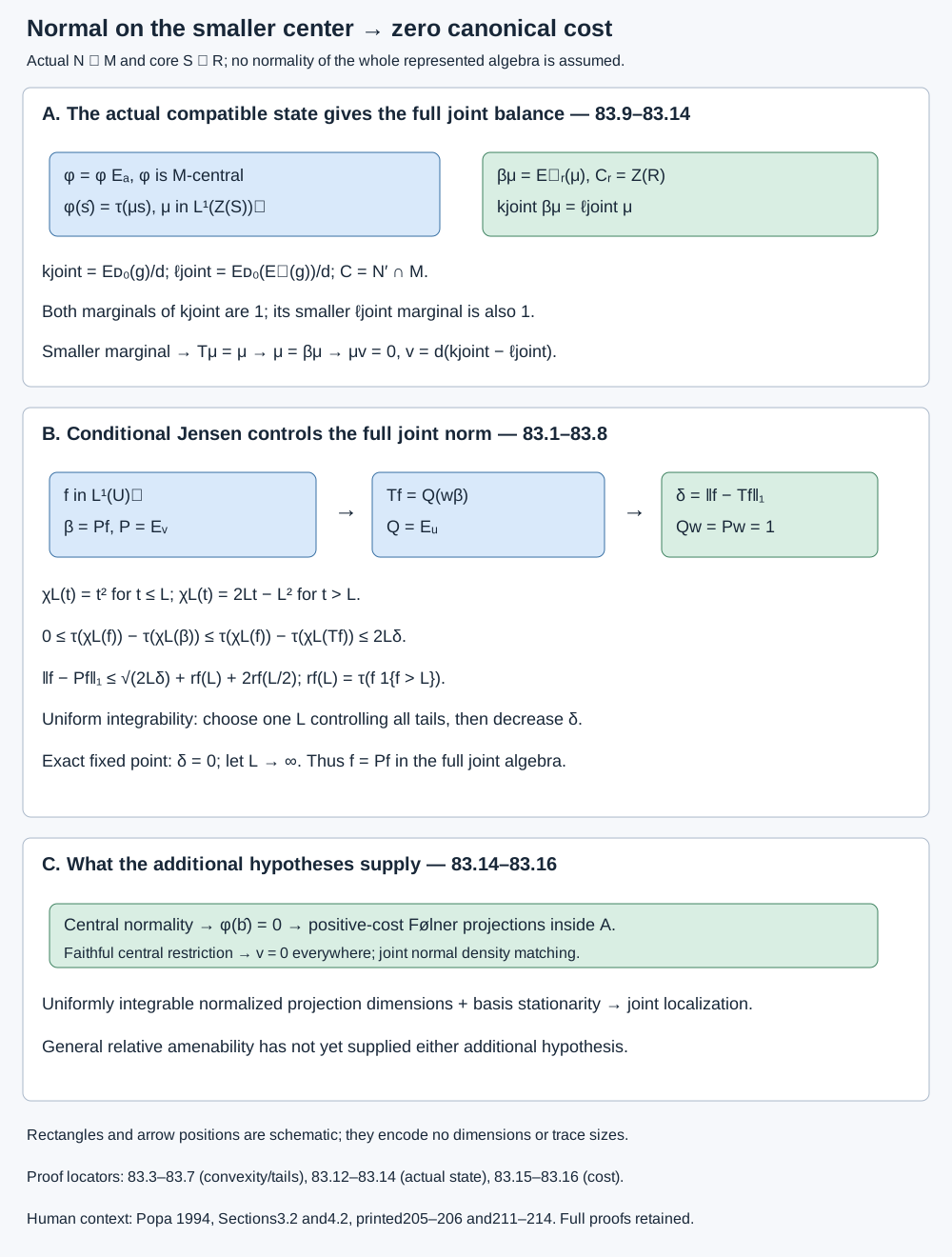
Figure 83.1. The first panel gives the maps and the exact normal balance (83.12). The second shows the conditional Jensen proof and tail bound, including the two-stage order of choosing parameters. The third states precisely which additional hypotheses produce zero cost. Positions are schematic, with no encoded traces or dimensions. Original editable source: normal-central-hypertraces-and-localization.py. The proof locators refer to this lesson. A three-dimensional scene would add no useful geometry.
Exercises with complete solutions
Exercise 83.1 — introductory
Suppose a mass-one density satisfies and . Give an explicit joint localization bound.
Solution. Equation (83.8) gives . The strict hypothesis gives a strict conclusion. The estimate concerns the full joint norm; it is not merely a scalar integral identity.
Exercise 83.2 — introductory
Use a four-point probability algebra whose points are pairs , each of mass . Let record , record , and let the weight matrix be . Compute , and the fixed densities for .
Solution. Both weight marginals equal one. Ordinary averages the two row coordinates, so on both columns. Weighted fixes that scalar, hence on both rows. A positive fixed density has ; these are exactly the positive elements of . This finite model illustrates the Markov theorem and is not claimed to be an actual Jones core.
Exercise 83.3 — intermediate
On the unit interval with Lebesgue probability measure, let . Is this mass-one family uniformly integrable? Contrast it with any family of mass-one densities bounded above by a common constant.
Solution. Each has integral one. For every fixed , choose ; then . The supremum of the tails therefore never tends to zero. In contrast, if every density is at most , the tails are zero for . This calculation concerns the tail condition alone and asserts no Følner properties for these densities.
Exercise 83.4 — intermediate
Explain the distinction between a hypertrace normal on , one faithful there, and one normal on all of . State exactly what each of the first two hypotheses gives in Theorem 83.5.
Solution. Normality on gives a positive integrable central density , potentially vanishing on a central region. The theorem gives and an annihilating state, hence selected positive-cost Følner projections. If that central restriction is also faithful, has support one; then everywhere and the full normal joint identity holds. Normality on all of is a stronger requirement than normality on its subalgebra ; the proof never assumes it. None of these conclusions identifies the full physical densities and .
Exercise 83.5 — advanced
For a family of mass-one dimensions assume for every . Find a sufficient numerical stationarity defect for , using (83.4).
Solution. Its two tail terms sum to at most . Choose ; this contributes at most . If , the square-root term is strictly below . Thus the total is strictly below . The choice of controls the whole family before its stationarity tolerance is set.
Exercise 83.6 — advanced
Why does alone fail to establish the cost conclusion? Identify the extra steps that the actual compatible state supplies.
Solution. A signed scalar integral can cancel. On two points of equal mass, take and ; the signed integral is zero while . Proposition 83.4 supplies the entire equality , tested against every bounded joint element. The smaller marginal and the positive fixed-point theorem then give . Substitution yields the operator identity . Commutativity makes , which is the absolute-cost assertion. No scalar cancellation was substituted for any of these steps.
Status and precise remaining hypothesis
The conditional Jensen estimate, quantitative joint localization, exact positive fixed points, actual normal central balance, central normality implication and uniform integrability route are proved here. General relative amenability has not supplied either extra hypothesis. The full original assignment remains active, including unrestricted exact full finite partition, common-stage or generating construction, central rounding and common-support basis, all finite pair and bicommutant comparisons, represented and opposite canonical traces, every original source clause, exercise, note and exact prerequisite.
Written by GPT-6.1 Sol (OpenAI), Ultra reasoning effort, October 2026. Public domain (CC0).