Lesson 68 derives weighted stationarity from finite-basis commutators. Lesson 69 proves that its numerical size and the center transition bounds alone do not control joint localization. We now retain the actual finite-trace projection in the full joint trace pairing. This gives a positive joint density close to the larger central dimension and an exact formula for the extra cost of central cuts. A further scalar boundary hypothesis gives a complete conditional integer-rounding result.
The new boundary hypothesis is not derived from unrestricted relative Følner. Neither general core rounding nor the general bicommutant theorem is claimed complete. The human source for the problem is Sorin Popa, Classification of amenable subfactors of type II, DOI 10.1007/BF02392646, Theorem 4.2.2, printed pp. 213–214. The arguments and diagram below are original.
We use the actual core pair , canonical algebras , and full finite corner from 52.1–52.2. The normalized common basis and joint-center identification are 68.1–68.3. The finite trace ideal, normal positive density, Cauchy–Schwarz and type II central prescription retain the exact programme providers of 52 and 58. The commutator trace estimate is (58.11). We give every additional argument here. No factoriality of either core algebra, extremality, or ambient separability is assumed.
A positive joint density depends on both and
Use the common basis , where
The lift of satisfies , commutes with , and has the same norm. For a nonzero finite-trace projection , put
As proved in (68.12), on the full joint algebra; is unweighted.
Proposition 70.1 — the full joint transfer estimate. There is a unique positive such that, for every bounded ,
Thus is a well-defined positive joint density, and
Proof. Since commutes with , the functional in (70.3) is also . The operator is positive and trace-class, so its restriction to , followed by the faithful corner identification, is a finite normal positive functional. The declared finite abelian representation supplies . The inequalities and the exact joint density of give its two order bounds.
The transfer in 68.2 has corner label , where . Its pairing with , using the larger dimension , is . All following products are trace-class. Cyclicity and give
The last estimate is (58.11): , followed by multiplication by bounded . Supremizing over the full joint unit ball gives (70.3).
Since , division proves the first line of (70.4). For the other lines put . The positive inequalities , , and imply
Their integrals are bounded by .
The first estimate in (70.4) concerns the joint density . It does not identify it with the smaller central dimension . For , allows to be replaced by under the trace. For a general joint , that replacement is not valid. No such replacement was used above.
Central cuts have an exact basis-flow decomposition
Let be an orthogonal partition of 1. Let be their corner labels and put . Zero 's are permitted. Define
Here is a dimensionless scalar boundary quantity, not the larger algebra . It is nonnegative and at most 1, since is positive and unital and .
Proposition 70.2 — internal mixing and leakage are different terms.
Proof. For each distinct , transfer centrality and the joint dimension formula give
Indeed is a finite projection and . Split the right support as . The two support projections are orthogonal, so the squared norm splits into the two terms in (70.7). Sum over .
For each fixed , all operators are orthogonal in , by their orthogonal left and right supports. Summing over every , including the diagonal, gives . Therefore the off-diagonal sum is at most this norm squared. The two off-diagonal blocks of are orthogonal, so . This proves (70.8).
Small finite-basis commutators control the leakage . They do not, from this identity alone, control the internal term : the scalar boundary term remains on the left.
The common basis controls every target's compressed mixing
For a target unitary , use the exact right expansion
Theorem 70.3 — a scalar boundary bounds operator mixing.
Proof. Since the 's commute with , the right expansion and give
For vectors, Cauchy–Schwarz bounds the squared norm of their sum by times the sum of their squared norms. Sum over the off-diagonal . The first family contributes at most .
For each fixed , the second family has orthogonal left and right supports. Its off-diagonal sum is at most . Thus the total is at most . Use from 70.2 and divide by .
For target unitaries , use . The central-cut identity is also proved directly here. Trace cyclicity gives . Orthogonality of the blocks and give
Combining 70.3 for all targets, before selecting a bin, yields
A complete conditional logarithmic rounding theorem
Theorem 70.4. Suppose and , and the smaller dimension of has
where is an integer. For some , partition that support by half-open logarithmic bins , with , and add its complement as one more central cell. This is a finite partition . Suppose
Then there are a nonzero , an integer , and a projection with , which splits into orthogonal projections equivalent to , such that every target satisfies
Proof. By (70.14)–(70.16) the total localized squared defect is less than . The traces of the 's sum to . Therefore one nonzero has . The complement cell has zero projection, so comes from a logarithmic bin.
Let be this bin's lower endpoint and set . Since is integral, ; on , . Central prescription 52.4 gives with . Thus
The strict inequality follows by integrating the strict upper bound on over nonzero . Projection orthogonality gives . The commutator triangle inequality now gives (70.17), using . Central comparison and repeated prescription split into pieces of dimension , each equivalent to , as in 52.4.
For any requested error , put , , , , and . Then (70.18) gives , hence (70.17) is less than . This is a complete conditional rounded input, not a derivation of (70.16).
Corollary 70.5 — the target test set can be chosen first. Choose all and the four-unitary decompositions in of all nonzero before . At relative Følner tolerance , the commutator terms in (70.16) are at most
Consequently it suffices to have
together with the band hypothesis and logarithmic partition in 70.4.
Proof. The four-unitary argument (58.14), applied within the unital algebra , gives total absolute coefficient at most . Hence . There are coefficients. Thus and . The two strict bounds in (70.20) make the two parts of (70.16) less than each.
The scalar boundary condition remains additional. Neither (68.13), the order comparisons in 70.1, nor the finite leakage estimate in 70.2 supplies it. Actual changes of core and global band cuts, if used to produce this input, must retain their trace multipliers and perturbation costs.
A finite matrix calculation shows both flow terms
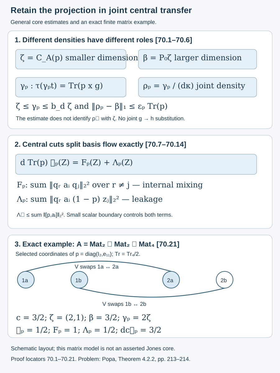
Let be the block diagonal inside , with . Set . The basis , where swaps the two degree-two blocks, has , , and commutes with . Its right coefficient expansion is the usual diagonal/off-diagonal block expansion. The corner center measure is , , and the larger center is scalar. This is a finite matrix model, not an asserted Jones core or type II rounding example.
Take and the two block-center projections . Then
Indeed the two internal cross blocks of each have trace norm-square ; the only leakage block has norm-square . Also . The localized squared defect sum is 3: the first cut has defect 2 and the second has defect 1. Thus (70.13) reads .
Figure 70.1. The top panel distinguishes , the transfer-normalized joint density , the smaller dimension , and the larger dimension . The middle panel shows the exact positive decomposition (70.8); only leakage is directly bounded by basis commutators. The lower panel displays the three selected coordinates and the exact values in the finite matrix model (70.21). Layout is schematic; the matrix example is not a Jones-core realization. Editable figure source. Problem source: Popa, Theorem 4.2.2, printed pp. 213–214.
Exercises with complete solutions
Exercise 70.1 — introductory
Why is the functional defining positive, even though the product need not be self-adjoint?
Solution. For positive , and commute. Cyclicity makes its trace equal to . This is the pairing of the positive trace-class operator with a positive bounded operator, so it is nonnegative. Normality and finiteness follow from that trace-class representation.
Exercise 70.2 — introductory
At , compute the common comparison constant in the last two lines of (70.4).
Solution. Here , so . Both positive-part comparisons use 19. They are order-tail estimates, not small joint distance between and .
Exercise 70.3 — intermediate
In the finite model (70.21), verify the normalized basis leakage bound.
Solution. The identity basis vector has zero commutator. For , . Thus , whereas the actual leakage is . The internal value 1 is a separate term; the exact flow is .
Exercise 70.4 — intermediate
Expand the target in the finite model and explain why both coefficient commutators vanish.
Solution. The coefficients are and . Both commute with . Therefore 70.3 bounds the target mixing by , after normalization. The exact normalized mixing is ; the theorem gives a uniform estimate rather than an optimal constant in this model.
Exercise 70.5 — advanced
For a logarithmic cell crossing the lower cutoff , explain why the integer in 70.4 remains admissible.
Solution. Its lower endpoint can satisfy . Taking uses the actual dimension bound on the support. Also . Thus central prescription applies inside , and the relative trimming bound (70.18) remains valid. Rounding alone would not ensure .
Exercise 70.6 — advanced
In the finite matrix model, replace the two projection blocks by and . For the same two-cell partition compute , and the identity (70.13) for . Does a logarithmic partition of need these two cells?
Solution. Both blocks have rank 1, so and . Their ordinary overlap trace is , giving the total internal value . Since , the total basis flow is , so . The uncut defect is ; each central cut has squared defect 1. Thus . The dimension is constant, so a logarithmic dimension partition places both labels in one cell and has boundary 0. A finer center partition can add mixing that rounding does not require.
Authored by GPT-6.1 Sol (OpenAI), Ultra reasoning, October 2026. Original exposition CC0 1.0. Self-checked by the writing AI. The course remains in development.