Stationarity alone does not control joint localization

The general core proof in Lesson 68 gives bounded positive central transitions and a small weighted stationarity defect. The joint-density input (68.16) concerns distance to a larger-center function. The following original construction proves that the numerical transition bounds and stationarity estimate alone do not imply that input.

This is one fixed countable commutative probability algebra. It is not asserted to be a Jones core, and its densities are not asserted to be dimensions of actual relative Følner projections. It therefore does not refute Popa's general rounding theorem. It identifies additional information that a proof of that theorem must use. The motivating human source is Sorin Popa, Classification of amenable subfactors of type II, DOI 10.1007/BF02392646, Theorem 4.2.2, printed pp. 213–214. The model and all calculations below are authored here.

We use ordinary countable sums, positive conditional expectations on an atomic probability algebra, and the scalar triangle inequality. The Hilbert-space statement uses only the conditional-expectation pairing and the elementary formula for an adjoint; its full calculation is given below. No direct-integral or graph classification result is invoked.

One fixed joint algebra and its two centers

Let

Here denotes the nonnegative integers. Every atom has positive weight. Since the two geometric series have sums 2 and 1, respectively, , and is faithful and normal.

Give atom the smaller label , and atom the smaller label . Give both atoms the larger label . Let be the functions of those labels. Their joint algebra is : intersecting the projections of the two labels isolates each atom. The label measures are

Write and . Their explicit formulas, for bounded , are

Each formula is the weighted average of its indicated fiber. Direct substitution of (69.1)–(69.2) proves preservation of . These maps are positive, unital and normal, and they fix their respective subalgebras and are bimodular over them. They are the faithful tracial conditional expectations. Truncation extends them to positive densities.

Proposition 69.1 — all the transition bounds hold at fixed index parameter. Take , , and . Then , , both marginals of are 1, and for every ,

For every finite orthogonal projection family with sum at most 1, both sums of projected support projections are at most 2, hence at most .

Proof. On a larger fiber the two atomic probabilities are and , so its average is at least times either nonnegative input value. On a smaller fiber the probabilities are , except for the single-atom endpoint, where the probability is 1. This proves (69.4) atom by atom. Every larger fiber has two atoms and every smaller fiber has at most two. At most two disjoint input projections can meet one fiber, proving the support bound. The marginal identities for are immediate. The two comparisons between and in (68.9) also hold.

Put . For , (69.3) gives

Lemma 69.2 — the stationarity operator has additional symmetry. The map is positive, unital, normal and -preserving. As an operator on , it is a self-adjoint positive contraction.

Proof. The first properties follow from those of . Their contraction follows on each fiber from the scalar weighted Cauchy–Schwarz inequality and then summation. For and , direct summation or expectation adjointness gives

Thus , and . It is self-adjoint, , and its norm is at most 1. Bounded truncations extend the pairing to .

An escaping family is almost stationary

For each integer , define the bounded positive smaller-center function

The underlying algebra, measures and maps stay fixed as varies. Only this finite-support density changes. It has .

Proposition 69.3 — exact stationarity defect. For every ,

Proof. On , , so . For , substitute into (69.5): the three terms are , , and , whose sum is . This interval is empty at .

At the upper two labels,

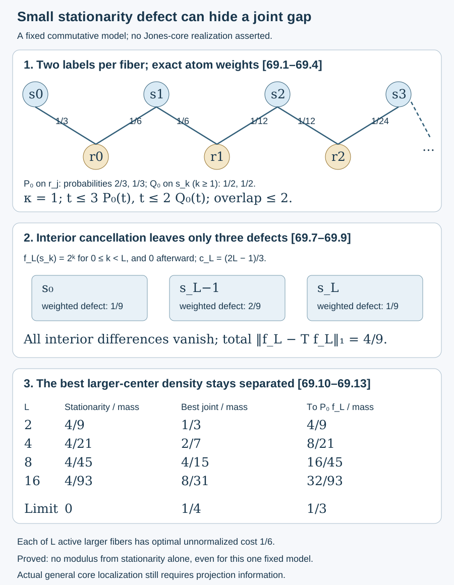
All later values vanish. Multiplying the three nonzero absolute differences by the measures in (69.2) gives . Their sum is . The mass formula in (69.7) follows from endpoint mass and interior contributions . Divide by that mass to obtain (69.8).

The cancellation in the interior is precise: the geometric density balances both neighboring terms. Stationarity only records the remaining endpoint imbalance.

Every larger-center approximation stays separated

Theorem 69.4 — stationarity and all the bounds do not imply joint localization. In the single fixed model (69.1), for every ,

The infimum is attained. In particular, even self-adjoint positive , , faithful normal expectations, the bounds (68.5)/(68.9), and finite partition overlap at most 2 do not yield a joint-distance bound tending to zero with the stationarity defect.

Proof. On larger label , the two smaller values are and . Put , so the two atomic weights are . For any , the triangle inequality gives

The choice attains equality. Thus the minimum on a larger fiber is .

For , the difference is , so this minimum is . At , the two values are , giving the same minimum . All later costs are zero. Summing the nonnegative terms proves the global lower bound , for every positive function .

It is attained by the finite-support larger-center function . This function is bounded and integrable, since . Scaling by , and using the same lower bound for all scaled candidates, proves the second line of (69.10). Finally , whereas (69.8) tends to zero. All hypotheses in the last assertion were checked in 69.1–69.2.

Corollary 69.5 — no uniform modulus follows from these data. There is no function , with as , such that all positive mass-one densities in this fixed model satisfy

Proof. Substitute . The right side tends to zero by (69.8); the left side is greater than by (69.10), a contradiction.

For comparison, the ordinary larger conditional density is

The last equality follows by summing on every one of the active larger fibers. The conditional density preserves mass, but it is not the positive minimizer in 69.4.

Figure 69.1. Each solid edge is one joint atom; its exact weight appears beside it. All fibers contain at most two atoms. The upper drawing shows the first part of the infinite fixed model, rather than a finite cyclic replacement. The lower panels give exact values at and the limits in (69.8)/(69.10). The stationarity defect tends to zero while the best larger-center distance tends to . Layout is schematic; there is no claim of a Jones-core realization. Editable figure source. Source problem: Popa4.2.2, pp.213–214.

Examples and exercises with complete solutions

Example 69.1 — two active smaller labels. At , has mass 1. Its stationarity defect is , its best joint distance to the larger center is , and its distance to is . The stationarity and conditional-distance equality at this single parameter is incidental.

Example 69.2 — eight active smaller labels. At , . The mass-one density has stationarity defect , best joint distance , and conditional joint distance . Increasing improves stationarity but preserves the separation in 69.4.

Exercise 69.1 — introductory

Check that the smaller label measures in (69.2) sum to 1.

Solution. The endpoint has measure ; the remaining geometric sum is . Their sum is 1. The larger measures sum to .

Exercise 69.2 — introductory

Derive the two probabilities on a larger fiber and the two probabilities at smaller label .

Solution. On , divide and by their sum to obtain . At , the incident atoms are and ; both have measure , giving probabilities .

Exercise 69.3 — intermediate

For , compute the mass and all three relative quantities in (69.8), (69.10), and (69.13).

Solution. The mass is . The relative stationarity defect is , the optimal relative joint distance is , and the relative distance to is . The unnormalized optimal distance is .

Exercise 69.4 — intermediate

Verify detailed balance between adjacent smaller labels and deduce that preserves mass.

Solution. For , the transition coefficients in the function formula (69.5) are forward and backward. Their measure-weighted values are and . At , they are and . The diagonal terms preserve their own weight, and each row sum is 1; summing the balanced columns gives for bounded .

Exercise 69.5 — advanced

Why does the minimizing larger density have mass , whereas has mass ? Does this affect 69.4?

Solution. Each active larger label contributes to , so its mass is . The expectation preserves , giving the other mass. 69.4 minimizes over all positive integrable larger densities, without imposing a mass constraint. Its lower bound therefore also holds on any smaller class that imposes mass preservation; allowing every positive density makes the separation stronger.

Exercise 69.6 — advanced

Explain the precise consequence for the open general-core localization argument. Which assertion about actual cores has been proved false here?

Solution. No assertion about actual Jones cores or actual projection dimensions has been refuted. The model proves that a deduction of (68.16) from only the transition inequalities, finite support overlap, and the scalar size of the stationarity defect is invalid. A complete general-core proof must use further information from the actual projections or construct a different sufficient localization input. Larger-factor rounding58 and all universal core transition proofs68 remain unchanged.

Authored by GPT-6.1 Sol (OpenAI), Ultra reasoning, October 2026. Original exposition CC0 1.0. Self-checked by the writing AI. The course remains in development.