Entropy bounds the central partition boundary

Lesson 70 proves a complete rounding theorem from a dimension band and a small scalar boundary. We now obtain the boundary from weighted stationarity inside a specified band. The estimate depends on the logarithmic spread of that band. It does not produce a band with this quantitative control from unrestricted relative Følner.

The motivating human source remains Sorin Popa, Classification of amenable subfactors of type II, DOI 10.1007/BF02392646, Theorem 4.2.2, printed pp. 213–214. The scalar estimates, finite-partition proof and diagram below are original. We use the actual centers, weighted expectations and normal trace formulas of 68.1–68.5, and the full projection and rounding proofs of 70.1–70.5. All their exact programme prerequisites remain in force. No direct-integral or joint tensor-product measure theorem is assumed.

A second route, Theorem 71.5 below, obtains the boundary directly from the actual joint distance with a constant independent of logarithmic spread. It uses a stronger input than stationarity. The two inputs and their remaining original construction obligations are stated separately.

A positive coupling on finite central partitions

Write , , and . Retain from Lesson 68, and put . Both marginal identities in (68.5) make positive, unital and -preserving.

For bounded , define the bilinear pairing

Lemma 71.1. For any finite orthogonal partition in , the numbers are nonnegative and satisfy

Proof. Both expectations are positive, and their outputs lie in the same abelian algebra . Their product is positive, so its trace is nonnegative. Summing one argument gives (71.2) by (71.1). No symmetry of is asserted. The second equality in (71.1) follows from expectation adjointness: .

For a finite-trace projection with dimension and , the boundary in (70.7) is exactly

Indeed , so taking in the other factor does not change the trace in (70.7).

An elementary entropy inequality controls absolute log differences

For positive real numbers , set

Lemma 71.2. This number is nonnegative, and

Proof. Put and , so . For , the exponential inequality , , gives . It proves both assertions and .

For , put . Then

Multiply by . This proves (71.5) without a bounded-ratio assumption on .

Stationarity supplies a logarithmic partition

Assume the actual projection dimension has a finite band

Thus on . For and , partition by the logarithmic intervals with lower endpoints , and add as one cell. Only finitely many intervals meet the band; call this partition .

Theorem 71.3. Some such shift has

In particular, the boundary can be made arbitrarily small when the band is fixed and stationarity tends to zero. The estimate uses no factoriality, extremality or ambient separability.

Proof for a finite spectral step function. First let with ; put and . Use the finite coupling of Lemma 71.1. Its outward loss is

Set on and on , so . Then

By the two equal marginals, the inside linear sum is

Expanding , and then subtracting this linear sum, gives the exact identity

Both subtracted terms are nonnegative. Lemma 71.2 and (71.9)–(71.10) therefore give . Apply (71.5), sum, and use scalar Cauchy–Schwarz and . The total absolute log cost satisfies

For two real log values, the probability that a uniform shift separates them into different width- cells is . To see this, translate one value to zero modulo : an interval of length equal to their separation crosses a boundary; it covers a fraction separation/ of a period until the separation reaches , after which every shift separates them.

The zero complement is always a separate cell. Its outward contribution is , while its incoming term is weighted by and vanishes. Thus

A shift with at most this average exists.

Passage to an arbitrary bounded dimension. Approximate uniformly by finite spectral step functions , equal to zero on , with all positive values in . Positivity and trace preservation make an contraction, so and .

The scalar spectral distribution of on under has at most countably many atoms. Except for a countable set of shifts, every bin endpoint has zero mass. At each such shift, the corresponding finitely many cell projections for converge in to those for . All cells remain in one fixed finite range of integer labels. The map is positive and -preserving, hence an contraction. Boundedness of and normality give convergence of every scalar term in (71.3). Therefore for almost every shift.

Every normalized boundary lies in , by (70.7). Bounded convergence passes (71.13) to the limit and proves (71.8). This finite-partition argument neither asserts a normal measure on nor uses a direct integral.

Rounding from controlled-spread stationarity

Corollary 71.4. Retain all actual target/basis/coefficient hypotheses of 70.4–70.5. Let the band satisfy (71.7) with the integer required there. For a desired scalar boundary tolerance , it suffices that

Then some logarithmic partition has . In particular choose , together with the independent commutator tolerance in (70.20); 70.4 supplies the rounded projection and its complete error estimate.

Proof. In (71.8), the three summands , , and are respectively less than under (71.14). Hence the boundary is less than . Theorem 70.4 selects and rounds a single nonzero bin using all target errors simultaneously.

This removes the separate boundary hypothesis once the band and the stated stationarity bound hold. The unrestricted problem is still to obtain an actual Følner projection with these simultaneous quantitative conditions, including every cost of low/high central cuts and changes of core. The spread is part of the hypothesis; it cannot be chosen after the stationarity tolerance without checking (71.14).

Joint distance supplies a partition without a spread factor

Weighted stationarity and joint distance are different inputs. The preceding proof estimates the boundary from and . We now use the actual joint distance

Here is bounded, positive and lies in ; its positive spectrum is contained in , with . For an actual projection it is the smaller canonical dimension used above. The estimate below does not involve .

Theorem 71.5. Some width- logarithmic shift, including the zero complement as a separate cell, satisfies

For an actual projection , . All expectations and measures are the inherited maps of Lesson 68. The theorem holds for nonfactor centers and makes no finite unit-capacity assumption.

Proof — the actual finite branches. By (68.9), for . Apply only the abelian branch construction 72.1–72.2 to with its faithful normal, -preserving expectation . It gives finitely many orthogonal projections , summing to one, with . There are at most branches. That branch construction is independent of the boundary estimates in this lesson.

Put , , and . The map , given by multiplication by , is a faithful normal *-isomorphism. Thus for a unique , extended by zero off . The resulting identities are

For the last line, apply to , apply to , and expand their product in the common abelian algebra . A branch coefficient off its support can be set to zero because both of its weights vanish there. The pair weight is ; it need not be symmetric or uniform.

Proof — the capped logarithm. For , let be when both are positive, one when exactly one is zero, and zero when both vanish. Then

If , use and , the latter following from . If , set . For , . For , the function is increasing: its derivative has positive numerator , since . Consequently . When one value is zero, (71.19) follows from ; both-zero terms vanish.

First take to be a finite spectral step function. The finitely many branch coefficients have a common finite spectral partition in . For each pair of their scalar values, the proportion of separating shifts is precisely , by the modulo- argument in Theorem 71.3, with zero always separate. Thus (71.18) can be integrated as a finite sum. Using (71.19) and the lattice triangle inequality around the actual gives

The first triangle contribution sums to one; the second sums to one and then uses . This is why both inherited weights must be retained.

For arbitrary bounded in the stated band, take finite spectral step approximations uniformly, preserving the zero complement and . The contraction of gives , and . Except at a countable set of shifts, all bin boundaries have zero mass for the scalar spectral distribution of . At every other shift, the finitely many cell projections converge in ; the number and range of integer bin labels have a common finite bound. Normality, boundedness and the contraction of give convergence of each boundary term, exactly as in the passage following (71.13). Every normalized boundary is between zero and one. Bounded convergence therefore passes (71.20) to the limit. A shift at most its average proves (71.17). This argument uses finite partitions and single-variable spectral distributions, with no direct-integral assumption.

A rounding input independent of the logarithmic spread

Corollary 71.6. Retain the actual projection, dimension band, targets and prior coefficient tests of 70.4–70.5. For any , it suffices that

Then some finite logarithmic partition has . In particular, choose

Here is the number of target unitaries, is the common basis size, and controls all target and coefficient-decomposition unitary commutators chosen before . Theorem 70.4 then selects one nonzero cell and prescribes an actual smaller canonical projection of dimension , with the target error bound (70.17) and relative trimming bound (70.18).

Proof. The strict inequality (71.21) and Theorem 71.5 give the boundary bound. Equation (70.19) bounds the prior coefficient and target contribution by . Equation (70.14) bounds the boundary contribution by . Their sum is strictly less than . The full simultaneous selection and feasible central prescription in 70.4 apply.

The new input is , rather than the stationarity defect . No implication from small to small joint distance has been added. Producing the required actual projection from unrestricted amenability remains a separate obligation. The selected label lies in ; the larger dimension is by (68.12). Equality with requires , and that stronger common-center support is not supplied by this estimate.

Three exact examples

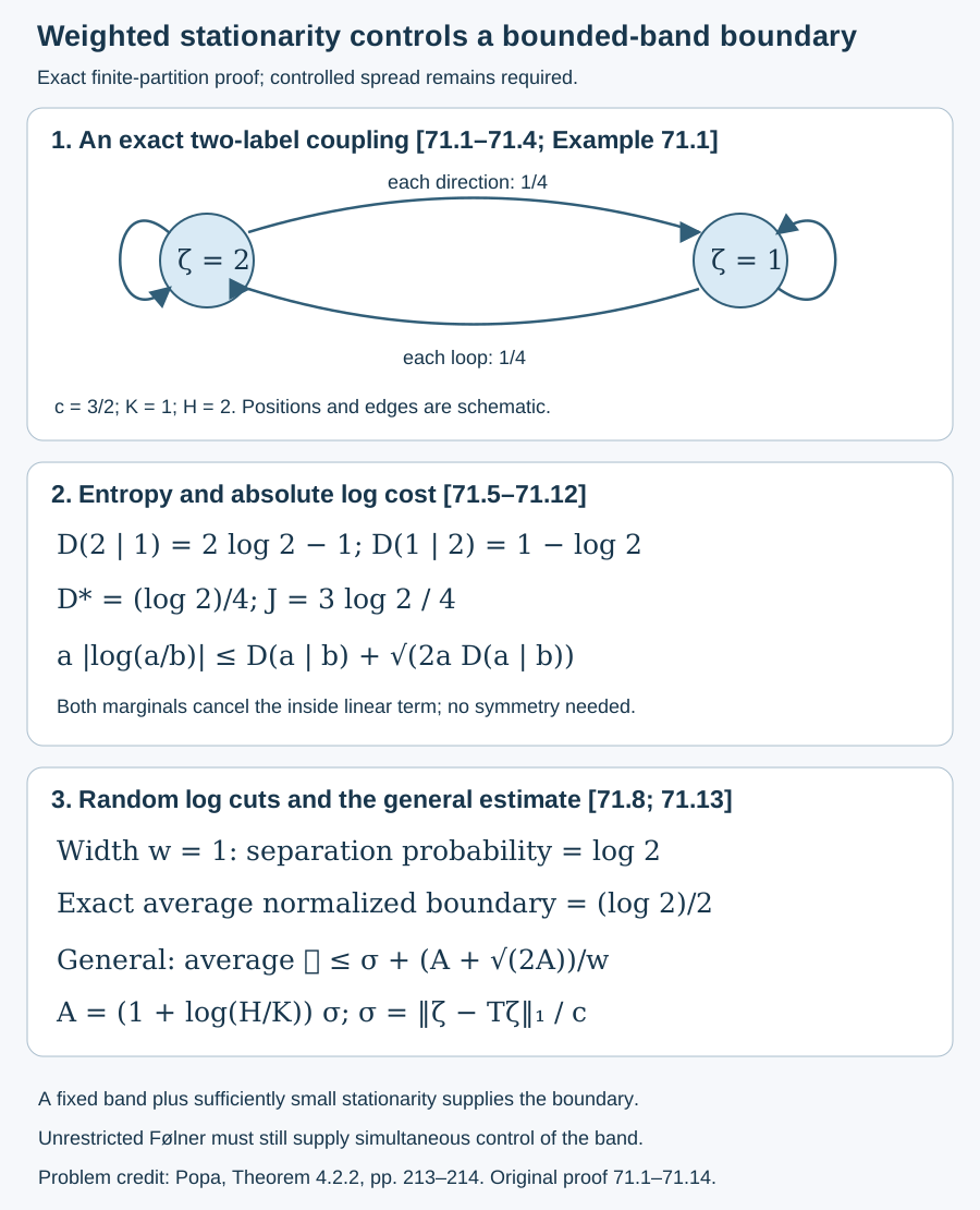
Example 71.1 — the two-label matrix model. In (70.21), , , , and every coupling entry is . Set . The inside entropy sum is , because and . There is no zero cell loss. The absolute log cost is ; the average normalized boundary is exactly , since . This is the finite matrix model already specified in Lesson 70, not a Jones-core realization.

Example 71.2 — a quantitative rounding input. Suppose , , , and the actual projection satisfies . Then , , and (71.8) gives

Here bounds the square-root term. If the prior target/coefficient unitary commutators also have tolerance , their total in (70.19) is at most . Thus the complete conditional rounding theorem applies. No assertion that unrestricted Følner supplies this particular band is made.

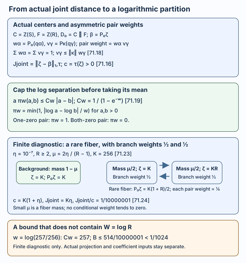
Example 71.3 — an arbitrarily wide band with fixed joint error. This is a finite commutative diagnostic, not an asserted Jones core or an actual projection construction. Let have three atoms: a background atom of mass , and two rare atoms of mass each. The algebra separates the background from the rare pair, while forgetting the distinction within that pair. Set , , ,

The ordinary branch weights are one on the background and on the rare fiber. Thus for , uniformly in . Small is the mass of a larger-center fiber, not a small conditional branch weight. The actual finite expectations give

Take , so exactly. Theorem 71.5 yields

This bound is uniform as becomes arbitrarily large. Indeed the rare labels are separated for every shift because , and their two off-diagonal pair weights are within that fiber. The exact boundary is

For an actual projection with the separate hypotheses , the bound is the required scalar budget in (71.22). Those physical hypotheses and its prior coefficient tests must still be established; this diagnostic does not supply them.

Figure 71.1. Both directions and both loops have coupling weight in Example 71.1. The two directional entropy costs sum to ; absolute log cost is . A width-one randomly shifted log partition separates the labels with probability , so its average normalized boundary is . The final panel states the exact general bound (71.8) and retains the controlled-band obligation. Coordinates are schematic. Editable figure source. Problem source: Popa, Theorem 4.2.2, pp. 213–214.

Figure 71.2. The inherited pair weights are those in (71.18). The capped-log bound (71.19) yields (71.17) without a spread factor. The three atoms illustrate exactly (71.23)–(71.26), with conditional rare-branch weights one half. Positions are schematic; this finite commutative diagnostic is not asserted to be a Jones core. Editable figure source. Human-source problem: Popa, Theorem 4.2.2, printed pp. 213–214; the new estimate is proved in Theorem 71.5.

Exercises with complete solutions

Exercise 71.1 — introductory

Why are both marginals needed in the finite-partition proof?

Solution. The row marginal sums outgoing to , and the column marginal sums incoming to . Together they convert the inside linear sum of to incoming zero-cell weight minus outward loss. This exact cancellation is used in (71.11). Symmetry is unnecessary.

Exercise 71.2 — introductory

Evaluate the two directional entropy costs for .

Solution. They are and , both nonnegative. Multiplying each by and adding cancels the constants and leaves .

Exercise 71.3 — intermediate

Why can the zero dimension be treated without taking its logarithm?

Solution. Define on . The outward coupling contribution is , bounded by stationarity outside the support. The incoming boundary contribution has coefficient . All logarithmic differences in use only positive , and both zero-cell terms in (71.11) are explicit.

Exercise 71.4 — intermediate

Derive the probability of separation when two log values differ by , by , and by .

Solution. Uniform translation modulo places a cell boundary between the values for a fraction , , and of shifts, respectively. These are the three values of . Equality at an endpoint has zero shift measure.

Exercise 71.5 — advanced

Verify all three terms of the strict bound (71.14).

Solution. Its first condition gives . The second gives . The third gives , hence . Adding yields the strict boundary bound , which is smaller than .

Exercise 71.6 — advanced

In Lesson 69's normalized escaping family, compute . Does this theorem supply a vanishing boundary at fixed width?

Solution. The positive density values have ratio , so . The stationarity defect is . Therefore

The bound in (71.8) does not tend to zero at fixed width. A finite band for each individual member is insufficient when its spread grows this way. No stationarity-only modulus refuted in Lesson 69 has been restored.

Exercise 71.7 — introductory

Check (71.19) when , when , and when .

Solution. The left sides are respectively zero, , and zero. The right sides are , , and zero. All inequalities hold because . No logarithm of zero is used.

Exercise 71.8 — intermediate

Explain why cannot be replaced by in (71.18).

Solution. The boundary pairs with , so their expansions use different coefficients. For example, conditional branch probabilities and branch values of equal to give . The outgoing pair weights are then and ; replacing both by changes the pairing. The proof only uses after the exact expansion.