Mixed Cauchy factors and admissible unique continuation

A complex double root cannot generally be split into two smooth first-order factors. The intact quadratic estimate controls exactly one derivative of its cofactor output. A polynomial reconstruction then recovers every derivative of the original function, while the local real-factor bracket estimate handles an oriented admissible normal. A fixed small dilation absorbs the complete operator errors before the weight grows.

The admissible set and the local simple/quadratic symbol geometry are proved in Admissible conormals for simple and double Cauchy factors. We receive the exact first-factor estimates from Exponential weights for first-order Cauchy factors, the intact quadratic estimate from A double-root estimate without choosing smooth roots, and the global bracket identities from Bracket control for first-order Cauchy factors. The scalar time estimate and the previous graph/cutoff framework are in Simple characteristic roots and local Cauchy uniqueness.

The exact transverse calculus interfaces are finite Weyl products (B5), Schwartz action (B6), change of quantization (B8a), left products (B8b), and continuity (B26) in When a moving symbol scale controls an operator. The scalar order-one lower bound is (P44)–(P45), at classical parameters and Sobolev exponent zero, in Positive quantization and sharp lower bounds. The scalar quadratic lower bound is the second line of (F5), with its complete proof in Sections 3–8, in When a nonnegative scalar symbol acquires a negative part. These precise interfaces retain their declared lower prerequisites. All receiving geometry, uniform metric bounds, finite remainders, polynomial reconstruction, graph approximation and support arguments are proved below.

The historical uniqueness theorem is Hörmander IV, Theorem 28.1.8 [H]. Equations marked E concern extensions, L concern localized real factors, C concern cofactor recovery, and N concern support normals and weak uniqueness.

1. Admissible exterior normals and the conclusions

1.1. Exact exterior-normal convention

The primary definition is Hörmander I, Definition 8.5.7, printed p. 300, PDF physical page 308. For a closed subset \(F\) of a \(C^2\) manifold \(X\), its exterior normal set is

The paragraph immediately after the definition establishes that this is a local definition: a support function defined on a neighborhood suffices. It also establishes that the support function may be replaced locally by an analytic quadratic function with the same differential. Thus the exterior set is exactly the set of smooth local support normals used by the cutoff proof. It is not defined as a closure.

Here is the replacement explicitly. In local coordinates let \(f_2\) be the quadratic Taylor polynomial of a \(C^2\) support function at \(z_0\). For fixed \(\lambda>0\), shrink the neighborhood until

Then \(g(z)=f_2(z)-\lambda|z-z_0|^2\) has \(dg(z_0)=df(z_0)\), and

Conversely a smooth local support function is \(C^2\), so it gives a member of (N1). Positive multiplication preserves \(N_e(F)\).

Printed p. 301, physical page 309, separately defines

Its notation \(\overline{N}(F)\) means the closure of this whole normal set in \(T^*X\setminus0\). The closure of the exterior set can likewise be written \(\overline{N_e(F)}\), but must not be confused with \(N_e(F)\) or with the whole set in (N3).

Hörmander IV, Theorem 28.1.8, printed p. 231, physical page 242, states the oriented exclusion

The symbol is \(\Gamma(p)\), whose admissibility conditions are Definition 28.1.7. The book does not replace \(N_e\) by a closure in the displayed theorem. Openness of \(\Gamma(p)\), proved in the admissibility lesson, yields the additional consequence

because \(T^*X\setminus(0\cup\Gamma(p))\) is closed relative to \(T^*X\setminus0\). This is a consequence of (N4), not a reinterpretation of its definition. Since \(\Gamma(p)\) can depend on the sign of the normal, (N4) does not by itself establish the same exclusion for \(N(F)\) or its whole closure.

1.2. The theorem and its weighted estimate

Let \(P=P_m+L\) be a differential operator of order \(m\ge1\) on \(X\), with smooth principal coefficients and locally bounded lower-order coefficients. Let

Theorem 1.1 (admissible unique continuation). Under the preceding hypotheses, (N6) implies the exclusion (N4), its limiting exterior-normal consequence (N5), and continuation across an oriented \(C^1\) surface with admissible conormal. The proof is completed in Section 5 after the mixed estimate is proved in Section 4.

The lower-order expression \(Lu\) is in \(L^2_{\mathrm{loc}}\), so (N6) implies \(P_m u\in L^2_{\mathrm{loc}}\). Products of bounded coefficients with the lower weak derivatives in (N6) are ordinary almost-everywhere products.

Fix an admissible exterior normal and put \(s=m-1\). After a smooth coordinate change and division by the nonzero leading normal coefficient, write the principal polynomial as monic in the normal frequency. Theorem 1.2 (mixed weighted estimate). On a fixed compact interior coordinate neighborhood \(K\), for all sufficiently small \(0<\epsilon\le\epsilon_0\) and all \(\tau\ge\tau_0\),

Here \(K\) lies in \(|t|<1/2\); its interior contains the eventual cutoff support. The constant \(C\) is uniform over the permitted small scales. Uniformity of \(C\) as \(\epsilon\downarrow0\), or an explicitly established scale with the absorption inequality (N15) below, is essential: \(C(\epsilon)\epsilon^2\) is not automatically small just because \(\epsilon\) is small. Section 4 proves this uniformity before the lower coefficients are absorbed.

There is no extra factor of \(\tau\) at the top derivative order in (N7). In particular, raising \(\tau\) alone cannot absorb arbitrary lower-order coefficients from this estimate. Hörmander IV's source powers are (28.1.37), printed p. 233, physical page 244.

2. Global separated extensions

The local factorization and the derivative condition used here are the conclusions of the admissibility lesson, Section 4, (4.6)–(4.8), and Section 5, (5.1). The real-root alternatives are (2.8). At a real simple root they give a nonpositive imaginary part, a signed bracket bound, or an absolute bracket bound. A nonreal simple root has a separated elliptic first factor. Every repeated group has degree two, nonreal center, and the full real-cone derivative condition below.

Let a monic homogeneous polynomial have, on a small real base and angular patch, a factorization into monic groups \[ p(z,\sigma,\eta)=\prod_{j=1}^J p_j(z,\sigma,\eta), \qquad \deg_\sigma p_j=m_j\in\{1,2\}. \tag{E.1} \] The simple groups are \(\sigma-a_j\). The double groups are \((\sigma-a_j)^2-q_j\), with \[ |\partial_\eta q_j|^2+|\eta|^{-2}|\partial_zq_j|^2 \le C|q_j|. \tag{E.2} \] At the central parameter \((0,\omega_0)\), each double group has its repeated nonreal root \(\lambda_j\); the simple groups have their corresponding roots \(\lambda_j\). Distinct groups have distinct \(\lambda_j\). Set \[ d_*=\min_{j\ne k}|\lambda_j-\lambda_k|>0 \tag{E.3} \] when there is more than one group. With one group the separation assertions below are unnecessary.

Choose a number \(\delta>0\) so small that \(4\delta<d_*\). For every nonreal center also require \(4\delta<|\operatorname{Im}\lambda_j|\). Shrinking the base and angular patches gives, for \(r=|\eta|\), \[ |a_j(z,\eta)-\lambda_jr|<\delta r,\qquad |q_j(z,\eta)|<\delta^2r^2 \tag{E.4} \] for a double group, and the first bound for a simple group. These follow from smoothness on the unit sphere and homogeneity; the double discriminant is zero at the central parameter. The patch is now fixed.

Use successively nested angular cones \(V_0\Subset V_1\Subset V_2\Subset V_3\) within that patch. The Fourier localizer is supported in \(V_0\), polynomial reconstruction will be used on \(V_1\), and all angular extension cutoffs are one on \(V_2\). Choose two nested real base cutoffs, equal to one on the smaller base neighborhood, whose supports lie in the original base patch. All coefficient agreement assertions refer to this smaller neighborhood.

For a simple group put, on \(V_3\), \[ a_j^{\,b}(z,\eta) =\beta(z)a_j(z,\eta)+(1-\beta(z))\lambda_jr. \tag{E.5} \] The term multiplied by \(\beta\) is extended by zero beyond its original base domain. This is smooth because the cutoff support lies strictly inside that domain. The first bound in (E.4) persists at every base point: \(|a_j^{\,b}-\lambda_jr|\le\delta r\). For a real central root, \(\lambda_j\) is real. Thus, if the original branch has imaginary part at most zero, (E.5) has imaginary part at most zero as well. For a nonreal central root its imaginary part has the same sign as \(\operatorname{Im}\lambda_j\) and modulus at least \((|\operatorname{Im}\lambda_j|-\delta)r\).

Extend a nonreal branch angularly by convex interpolation between \(a_j^{\,b}\) and \(s_ji r\), where \(s_j=\operatorname{sign}\operatorname{Im}\lambda_j\). Both imaginary parts have that sign and a common positive lower bound times \(r\); the bound therefore persists under interpolation. Extend a real-central branch with an angular cutoff to the real function \(\lambda_jr\). In the microhyperbolic branch its imaginary part remains at most zero globally. In either local bracket branch the angular extension is only required to be smooth with bounded symbol seminorms. The bracket hypothesis will be used on its original smaller patch, through the separate receiving localization proof.

For a double group choose a real cutoff \(\chi(z,\eta)\) supported in the original base and angular patch, equal to one on the coefficient-agreement region, with \[ |\partial_\eta\chi|\le C/r,\qquad |\partial_z\chi|\le C. \tag{E.6} \] Define \(q_j^{\,e}=\chi^2q_j\), extending the cut-off term by zero. On \(r\ge1\), the exact product rule gives \[ \begin{split} |\partial_\eta q_j^{\,e}|^2 &\le 2\chi^4|\partial_\eta q_j|^2 +8\chi^2|\partial_\eta\chi|^2|q_j|^2,\\ r^{-2}|\partial_zq_j^{\,e}|^2 &\le 2\chi^4r^{-2}|\partial_zq_j|^2 +8\chi^2r^{-2}|\partial_z\chi|^2|q_j|^2. \end{split} \tag{E.7} \] Since \(|q_j|\le\delta^2r^2\) and \(0\le\chi\le1\), each right side is bounded by \(C\chi^2|q_j|=C|q_j^{\,e}|\). This proves the derivative hypothesis even at zeros and along the entire cutoff transition. No derivative of a square root is used.

Extend the center by (E.5), and then angularly by the same-sign interpolation just described. The base and angular center cutoffs can be wider than those for \(q_j^{\,e}\). There is a \(c_j>0\), uniform over every base point, such that \[ |\operatorname{Im}a_j^{\,e}|\ge c_jr,\qquad |q_j^{\,e}|\le\delta^2r^2 . \tag{E.8} \] Shrink the original choice of \(\delta\) once more so that \(\delta^2\le c_j^2/2\) for each double group. For real \(\sigma\), \[ \begin{split} |(\sigma-a_j^{\,e})^2-q_j^{\,e}| &\ge|\sigma-a_j^{\,e}|^2-|q_j^{\,e}|\\ &\ge\tfrac12\big((\sigma-\operatorname{Re}a_j^{\,e})^2 +c_j^2r^2\big)\\ &\ge c'_j(\sigma^2+r^2). \end{split} \tag{E.9} \] For the last inequality use \(|\operatorname{Re}a_j^{\,e}|\le Cr\): \(\sigma^2\le2(\sigma-\operatorname{Re}a_j^{\,e})^2+2C^2r^2\). This proves full real-frequency quadratic ellipticity. The same imaginary lower bound proves the frozen-time center hypothesis of the intact quadratic estimate.

Multiply each extended center by a smooth radial cutoff equal to one above a fixed radius and zero near \(\eta=0\), and include its square in the discriminant cutoff. All symbols are then smooth ordinary \(S^1\) or \(S^2\) symbols globally. In the bounded radial region their symbol bounds give the additive constants in \[ \begin{gathered} |\eta|\le C(|\operatorname{Im}a_j^{\,e}(0,x,\eta)|+1),\\ 1+\sigma^2+|\eta|^2 \le C\big(|(\sigma-a_j^{\,e})^2-q_j^{\,e}|+1\big),\\ |\partial_\eta q_j^{\,e}|^2+ \langle\eta\rangle^{-2}|\partial_zq_j^{\,e}|^2 \le C(|q_j^{\,e}|+\langle\eta\rangle). \end{gathered} \tag{E.10} \] To justify the second line in the bounded radial region, all coefficient values there are uniformly bounded. For \(|\sigma|\) above a fixed bound the monic quadratic has modulus at least \(\sigma^2/2\); below that bound the added \(1\) bounds the entire left side after enlarging \(C\).

On \(V_1\), at high frequency, every extended simple root lies within \(\delta r\) of \(\lambda_jr\). Every root of an extended double group lies within \(2\delta r\) of \(\lambda_jr\), because its center displacement is at most \(\delta r\) and either square root of its discriminant has modulus at most \(\delta r\). These disks are pairwise disjoint by \(4\delta<d_*\). This holds for every real base point, including outside the original base patch. Hence the extended monic groups are pairwise coprime on the whole wider interpolation cone, for every base point. There is no separation assertion outside this cone.

The construction used central constant cluster centers and cut the discriminant to zero. Convex interpolation between two complex discriminants would not prove (E.2): cancellation could produce a zero with a nonzero derivative. That interpolation is unnecessary here. All extensions agree exactly with the original groups on the input localization region. ∎

3. Full finite localization and the real-factor estimate

3 — 1. Slow classes and their uniform metric

Write \(L(\eta)=\langle\eta\rangle\), \(D=-i\partial\), and fix \(0<\epsilon\leq1\). A family \(f_\epsilon(t,x,\eta)\) belongs to \(S_\epsilon^r\) if \[ |\partial_t^\ell\partial_x^\beta\partial_\eta^\alpha f_\epsilon| \leq C_{\ell\beta\alpha}\epsilon^{\ell+|\beta|}L^{r-|\alpha|}. \tag{L1} \] All family bounds are independent of \(\epsilon\). A prefactor \(\epsilon^a S_\epsilon^r\) is an additional prefactor. An undilated smooth ordinary order-\(r\) symbol, with globally bounded base derivatives, evaluated at \((\epsilon t,\epsilon x,\eta)\), satisfies (L1).

The transverse metric and its symplectic dual and Planck parameter are \[ g_{\epsilon,(x,\eta)}=\epsilon^2|dx|^2+L^{-2}|d\eta|^2,\qquad g_\epsilon^\sigma=L^2|dx|^2+\epsilon^{-2}|d\eta|^2,\qquad h_\epsilon=\epsilon/L. \tag{L2} \] At fixed \(t\), (L1) is equivalent to boundedness in \(S(L^r,g_\epsilon)\). Its positive time derivatives are additional parameter bounds.

For the structural checks, \(g_{\epsilon,X}(Y-X)\leq1/16\) implies \(|\eta_Y-\eta_X|\leq L(\eta_X)/4\). The elementary Lipschitz inequality for \(L\) gives \(3/4\leq L(\eta_Y)/L(\eta_X)\leq5/4\), so local comparisons have common constants. Put \(d_Y=g_{\epsilon,Y}^\sigma(X-Y)\). Then \(|\eta_X-\eta_Y|\leq\epsilon\sqrt{d_Y}\), and, since both \(L\)'s are at least one, \[ L(\eta_X)/L(\eta_Y),\quad L(\eta_Y)/L(\eta_X) \leq1+|\eta_X-\eta_Y|\leq1+\sqrt{d_Y}. \tag{L3} \] This proves symplectic temperateness of the metrics and weights \(L^r\) with uniform constants; the \(dx\) coefficients cause no extra ratio. The uncertainty inequality \(g_\epsilon\leq g_\epsilon^\sigma\) follows from \(\epsilon\leq1\leq L\), and direct division gives \(h_\epsilon\) in (L2). Thus the selected calculus, continuity, and quadratic positivity theorems have common structural constants. Replacing the \(dx\) coefficient by \(\epsilon^{-2}\) would not yield these small remainders.

Their finite interfaces give, for \(f_\epsilon\in S_\epsilon^r\) and \(g_\epsilon\in S_\epsilon^{r'}\), \[ f_\epsilon\#g_\epsilon-\sum_{\nu<N}C_\nu(f_\epsilon,g_\epsilon) \in\epsilon^N S_\epsilon^{r+r'-N}. \tag{L4} \] The same statement holds for left composition and its differential terms. Either conversion between left and Weyl quantization, through degree \(N-1\), has remainder \(\epsilon^N S_\epsilon^{r-N}\). Each contraction has one base and one frequency derivative, hence a factor \(\epsilon L^{-1}\). These are actual full finite remainders, with every prescribed output seminorm controlled by finitely many input seminorms.

Parameter differentiation commutes with the exact product and conversion: first differentiate the compact approximants in their oscillatory integrals, then pass to the bounded-symbol limit by the provider's continuity. The \(\ell\)-th derivative of a product is the finite Leibniz sum. Its two input prefactors multiply to \(\epsilon^\ell\); apply the same remainder theorem to every pair and subtract the differentiated finite terms. Hence every positive time derivative of every full remainder in (L4) retains the extra factor \(\epsilon^\ell\). No convergent infinite symbolic expansion is needed.

3 — 2. Time polynomials and the weighted receiving norm

For an integer \(q\geq0\), let \(\mathcal T_{\epsilon,q}\) consist of \[ R_\epsilon=\sum_{j=0}^{q}\operatorname{Op}_L(d_{\epsilon,j}(t))D_t^j, \qquad d_{\epsilon,j}\in S_\epsilon^{q-j}. \tag{L5} \] The classes here include full coefficient symbols. We also use a separate maximal time degree \(q\) and coefficient orders \(p-j\), allowing negative transverse orders when \(p<q\).

Finite products of slow monic factors, including intact quadratics, of total degree \(q\) have the form (L5). The exact normal-ordering rule is \[ D_t^a C(t)=\sum_{\ell=0}^{a}{a\choose\ell} (-i)^\ell(\partial_t^\ell C(t))D_t^{a-\ell}. \tag{L6} \] Each time differentiation lowers the time degree and adds a factor \(\epsilon\); it never increases transverse order. The allowed coefficient order, total degree minus remaining time degree, therefore bounds every resulting term. Transverse products preserve that order and all the time bounds by (L4) with \(N=0\). This proves (L5) by finite induction. The top monic coefficient is exactly one.

Let \(J=(-1/2,1/2)\), \(\phi=t+t^2/2\), \(W=e^{\tau\phi}\), and \(\tau\geq1\). For compact-time smooth input set \[ H_s(u)^2=N_s(u)=\sum_{j+|\beta|\leq s} \tau^{2(s-j-|\beta|)}\|W D_t^jD_x^\beta u\|_2^2. \tag{L7} \] If an operator has maximal time degree \(q\leq s\) and coefficient orders \(p-j\), where \(p\leq s\), then \[ \|WR_\epsilon u\|_2\leq C H_s(u). \tag{L8} \] Indeed an order-\(a\) transverse symbol maps \(H_x^k\) to \(L_x^2\) uniformly for an integer \(k\geq\max(a,0)\). To prove this from the selected interface, its left composition on the right with \(L(D_x)^{-k}\) has exact symbol \(d(x,\eta)L(\eta)^{-k}\), because the right multiplier has no \(x\) dependence. That symbol has order at most zero; conversion and (B26) bound it. For \(a<0\), take \(k=0\). Plancherel controls \(H^k_x\) by the finite transverse derivatives through degree \(k\). Apply this at every \(t\) to \(WD_t^j u\). Since \(W\) commutes with every transverse coefficient, and \(k=\max(\lceil p-j\rceil,0)\) satisfies \(j+k\leq s\), all these terms occur in (L7) with weights at least one. The finite sum and time integration prove (L8), including any additional prefactor \(\epsilon^a\).

Weight conjugation is also exact: \[ WR_\epsilon W^{-1} =\sum_j\operatorname{Op}_L(d_{\epsilon,j})(D_t+i\tau\phi')^j. \tag{L9} \] The power is an operator power. If it is written as \(\sum_{\ell=0}^j p_{j\ell}(t,\tau)D_t^\ell\), then \[ p_{0,0}=1,\qquad p_{j+1,\ell}=p_{j,\ell-1}-i\partial_t p_{j\ell} +i\tau\phi'p_{j\ell}. \tag{L10} \] Absent coefficients are zero. Thus \(p_{jj}=1\), and every fixed time derivative is bounded on \(J\) by \(C_{j,\nu}\tau^{j-\ell}\). This retains the derivatives of \(\phi'\): the zeroth coefficient of the square, for example, is \(\tau\phi''-\tau^2(\phi')^2\). The corresponding expansions with \(D_t-i\tau\phi'\) give \[ N_s(u)\asymp\sum_{\ell+|\beta|\leq s} \tau^{2(s-\ell-|\beta|)} \|D_t^\ell D_x^\beta(Wu)\|_2^2. \tag{L11} \] To check the powers, the factor \(\tau^{j-\ell}\) combines with the original weight \(\tau^{s-j-|\beta|}\) to produce exactly \(\tau^{s-\ell-|\beta|}\). The inverse expansion proves the other inequality. All constants in (L8)–(L11) are independent of \(\tau,\epsilon\).

3 — 3. The full finite support-remainder lemma

Let \(\theta(\eta)\in S^0\) be a fixed Fourier localizer supported in a smaller angular cone and away from the radial region where the homogeneous root is undefined. Let \(\psi(t,x)\) be smooth and compactly supported in the original local base chart; put \(\psi_\epsilon(t,x)=\psi(\epsilon t,\epsilon x)\). Choose fixed wider neighborhoods inside the root patch. Write \[ \mathcal S_\epsilon=\{(t,x,\eta): (\epsilon t,\epsilon x)\in\operatorname{supp}\psi,\ \eta\in\operatorname{supp}\theta\}. \tag{L12} \] For a monic cofactor, this is its projected principal support after right localization: its top time coefficient is one, so zeros of some other coefficients do not reduce the union of the coefficient supports.

Lemma. Suppose \(c_\epsilon\in\epsilon^aS_\epsilon^r\) vanishes on a neighborhood of \(\mathcal S_\epsilon\). Let \(R_\epsilon\in\mathcal T_{\epsilon,q}\), and fix \(N\geq1\). There is an exact identity of full operators \[ c_\epsilon^wR_\epsilon\Theta\psi_\epsilon =\epsilon^{a+N}\sum_{k=0}^{q} \operatorname{Op}_L(e_{\epsilon,N,k})D_t^k,\qquad e_{\epsilon,N,k}\in S_\epsilon^{r+q-k-N}. \tag{L13} \] The full remainder retains time degree at most \(q\), and every positive time derivative of its coefficient retains the factor specified in (L1). If \(q\leq s\) and \(r+q-N\leq s\), then \[ \|Wc_\epsilon^wR_\epsilon\Theta\psi_\epsilon u\|_2 \leq C_N\epsilon^{a+N}H_s(u). \tag{L14} \] No spatial compactness of the output is assumed.

Proof. Remove the explicit prefactor \(\epsilon^a\). Normal-order \(R\) and move each \(D_t^j\) through \(\psi_\epsilon\) using (L6); \(\Theta\) commutes with time differentiation. A term with \(\ell\) derivatives on \(\psi_\epsilon\) has time degree \(k=j-\ell\). Its transverse composite is \[ c_\epsilon^w\operatorname{Op}_L(d_{\epsilon,j}) \theta(D_x)M_{\partial_t^\ell\psi_\epsilon}. \tag{L15} \] Convert the first factor to left quantization and expand these three compositions through total contraction degree \(N-1\). This is a finite operation: a term already of degree \(b<N\) is next expanded only through degree \(N-b-1\); its full remainder is taken at degree \(N-b\). An earlier full remainder is composed with the remaining factors by the \(N=0\) continuity statement. Induction proves that the resulting full remainder lies in \[ \epsilon^{N+\ell}S_\epsilon^{r+q-j-N}. \tag{L16} \] Here \(\partial_t^\ell\psi_\epsilon\) contributes \(\epsilon^\ell\), and each contraction contributes \(\epsilon L^{-1}\).

Each retained local differential monomial contains derivatives of all four factors, evaluated at the same phase point. Nonzero derivatives of \(\theta\) and \(\partial_t^\ell\psi_\epsilon\) put that point in \(\mathcal S_\epsilon\). Every derivative of \(c_\epsilon\) vanishes there by its neighborhood vanishing. Thus every retained monomial is identically zero: only (L16) remains. Since \(k=j-\ell\), its order is \(r+q-k-N-\ell\), no larger than the asserted order in (L13). Divide by \(\epsilon^N\); the remaining \(\epsilon^\ell\) is bounded by one. The differentiated finite remainder estimates already proved preserve the same bounds after all time derivatives. Sum the finitely many terms and restore \(\epsilon^a\). This proves (L13). Apply (L8) with separate maximal time degree \(q\) and coefficient order parameter \(p=r+q-N\) to obtain (L14). If \(p<0\), all coefficients have nonpositive transverse order while \(q\leq s\) still bounds their time derivatives. \(\square\)

Only the leading symbol of an arbitrary operator would be insufficient: the proof uses full slow coefficient bounds and the exact right localization. The transverse order loss in (L13) does not remove top time derivatives when \(q+r-N<q\).

3 — 4. Exact first-factor symbols after a slow extension

Choose an arbitrary bounded smooth global extension \(a(y,\eta)\in S^1\) of the local root, equal to it on a wider neighborhood of the undilated support in (L12), at the relevant high frequencies. No global bracket condition on the extension is assumed. Put \[ A=\operatorname{Op}_L a(\epsilon t,\epsilon x,\eta),\quad K=(A-A^*)/(2i),\quad B=[A^*,A]+[D_t,A^*-A]. \tag{L17} \] These are transverse operators with \(t\) as a parameter; \(B\) contains no remaining \(D_t\). In undilated variables define \[ \iota=\operatorname{Im}a,\qquad b=2\{\operatorname{Re}a,\iota\}_{x,\eta}-2\partial_t\iota. \tag{L18} \] With the transverse bracket \(f_\eta g_x-f_xg_\eta\) and the same convention in the time-frequency pair, (L18) is the full bracket \(\{\overline{\sigma-a},\sigma-a\}/i\).

The exact Weyl symbols defined by \(K=k_\epsilon^w\) and \(B=\epsilon\beta_\epsilon^w\) are real and satisfy \[ \begin{split} k_\epsilon&=\iota(\epsilon t,\epsilon x,\eta)+\epsilon r_{\epsilon,0}, &r_{\epsilon,0}&\in S_\epsilon^0,\\ \beta_\epsilon&=b(\epsilon t,\epsilon x,\eta)+\epsilon r_{\epsilon,1}, &r_{\epsilon,1}&\in S_\epsilon^0. \end{split} \tag{L19} \] Thus \(k_\epsilon,\beta_\epsilon\) are uniformly in \(S_\epsilon^1\), and their errors have all the positive-time-derivative bounds.

To prove (L19), the exact Weyl symbol of \(A\) is \(a_w=a_\epsilon+\epsilon S_\epsilon^0\) by the finite \(N=1\) conversion. Weyl adjunction is complex conjugation, so \(k_\epsilon=\operatorname{Im}a_w\). The exact symbol of \([D_t,-2iK]\) is \(-2\partial_t k_\epsilon\), because \([D_t,K]=-i(\partial_t k_\epsilon)^w\). The scalar Weyl commutator has first symbol \(\{\overline a_w,a_w\}/i=2\{\operatorname{Re}a_w,\operatorname{Im}a_w\}\). Its degree-zero and degree-two terms cancel. Its full degree-three remainder is \(\epsilon^3 S_\epsilon^{-1}\), using (L4) on two order-one symbols. Replacing a leading factor by its \(\epsilon S_\epsilon^0\) correction in the first bracket adds another slow base derivative and gives \(\epsilon^2 S_\epsilon^0\). The time derivative of that correction has this same class. The leading terms are \(\epsilon b_\epsilon\); division by \(\epsilon\) proves the second line of (L19). This finite computation retains the entire operator remainder.

For the simple-factor application let \[ \begin{gathered} s=m-1,\quad q=s,\quad w=R_\epsilon\Theta\psi_\epsilon u,\quad v=Ww, \quad X=\|v\|_2,\\ T=D_t+i\tau\phi'-A,\qquad E=\|Tv\|_2,\qquad V=\|T^*v\|_2. \end{gathered} \tag{L20} \] The argument also works for \(q\leq s\). Take \(u\in C_c^\infty(J\times\mathbb R^d)\), and take \(\psi_\epsilon=1\) near its actual support when that equality is needed by the later localization. For the estimates it is enough to use the displayed localized input. By transverse Schwartz action and the finite time polynomial, \(w,v\) are Schwartz in \(x\) and compactly supported in time in \(J\). Their spatial outputs may have arbitrarily long tails. Exact Leibniz expansion for \(\psi_\epsilon\), followed by (L8), gives \[ X\leq C_R H_s(u). \tag{L21} \]

Without any bracket hypothesis, direct expansion and compact-time integration by parts give \[ [T^*,T]=2\tau+B,\qquad E^2=V^2+2\tau X^2+(Bv,v). \tag{L22} \] The inner product is linear in the first variable. In the first identity \(A\) commutes with the time-only \(\phi'\), and \([D_t,i\tau\phi']=\tau\phi''=\tau\). Put \[ M^2=\max\{0,-(Bv,v)\}. \tag{L23} \] Then \[ V\leq(E^2+M^2)^{1/2}\leq E+M,\qquad \|Kv\|_2\leq E+\tfrac12M+\tfrac32\tau X. \tag{L24} \] For the second inequality use \(T-T^*=2i(\tau\phi'-K)\), the first inequality, and \(\sup_J|\phi'|=3/2\). The extended operators and the same input \(v\) occur throughout.

Choose a real nonnegative wider cutoff \(\kappa_\epsilon=\kappa(\epsilon t,\epsilon x,\eta)\), with \(0\leq\kappa\leq1\), equal to one on a neighborhood of the undilated support in (L12), and supported strictly inside the region of root agreement and the local bracket condition. Fixed angular and radial choices and a fixed slow base cutoff ensure \(\kappa_\epsilon\in S_\epsilon^0\) uniformly, including time derivatives. This compresses symbols; it does not modify the root to assert a bracket bound at its cutoff edge.

3 — 5. The local signed branch

Assume on \(\operatorname{supp}\kappa\) that \[ b+C_0\iota+C_1\geq0,\qquad C_1\geq0. \tag{L25} \] Here \(C_0\) may be real. The signed L054 alternative has \(C_0\geq0,C_1=0\). The globally smooth symbol \[ p_\epsilon=\epsilon\kappa_\epsilon (b+C_0\iota+C_1)(\epsilon t,\epsilon x,\eta)\geq0 \tag{L26} \] is in \(\epsilon S_\epsilon^1\), hence a uniformly bounded ordinary order-one family. Apply (P44)–(P45) to its left quantization. Conversion to Weyl costs a full \(\epsilon^2S_\epsilon^0\) remainder, which is controlled by (B26). Thus, first at each time and then by integration, \[ (p_\epsilon^w v,v)\geq-CX^2. \tag{L27} \] One could keep a factor \(\epsilon\) on the right; the uniform bound suffices.

The exact Weyl symbol of \(P_\epsilon=B+\epsilon C_0K\) is \(\epsilon(\beta_\epsilon+C_0k_\epsilon)\). The following decomposition is exact: \[ \begin{split} P_\epsilon&=p_\epsilon^w+c_\epsilon^w+d_\epsilon^w,\\ c_\epsilon&=\epsilon(1-\kappa_\epsilon) (\beta_\epsilon+C_0k_\epsilon),\\ d_\epsilon&=\epsilon\kappa_\epsilon [\beta_\epsilon+C_0k_\epsilon-(b+C_0\iota+C_1)_\epsilon]. \end{split} \tag{L28} \] The first error \(c_\epsilon\in\epsilon S_\epsilon^1\) vanishes on a neighborhood of \(\mathcal S_\epsilon\). The second lies in \(\epsilon S_\epsilon^0\): its constant contribution is \(-\epsilon C_1\kappa_\epsilon\), and its remaining terms are \(\epsilon^2S_\epsilon^0\) by (L19). It is \(L^2\) bounded with norm \(C\epsilon\).

The full support lemma, with \(a=1,r=1,N=1,q=s\), gives \[ \|c_\epsilon^w v\|_2 =\|Wc_\epsilon^wR_\epsilon\Theta\psi_\epsilon u\|_2 \leq C\epsilon^2H_s(u). \tag{L29} \] By (L21), its form is bounded by \(C\epsilon^2N_s(u)\). Combining the three terms in (L28) with (L27) gives \[ (Bv,v)+\epsilon C_0(Kv,v) \geq-CX^2-C\epsilon^2N_s(u). \tag{L30} \] If the \(B\) form is negative, apply Cauchy–Schwarz to the \(K\) form. If it is nonnegative, \(M=0\). Both cases yield \[ M^2\leq\epsilon|C_0|\,\|Kv\|_2X+CX^2+C\epsilon^2N_s(u). \tag{L31} \] This local receiving inequality includes the entire spatial tail error and requires no global signed bracket bound.

3 — 6. The local absolute branch and its full quadratic symbol

Assume instead on \(\operatorname{supp}\kappa\) that \[ |b|\leq C_0|\iota|+C_1,\qquad C_0,C_1\geq0. \tag{L32} \] By (L19) there is a fixed \(D\), independent of \(0<\epsilon\leq1\), such that \[ |\beta_\epsilon|\leq C_0|k_\epsilon|+D \quad\text{on }\operatorname{supp}\kappa_\epsilon. \tag{L33} \] Indeed both normalized correction symbols are bounded, and \(|\iota_\epsilon|\leq|k_\epsilon|+\epsilon|r_{\epsilon,0}|\).

Form the exact real Weyl symbol \[ F_\epsilon=\beta_\epsilon\#\beta_\epsilon -2C_0^2k_\epsilon\#k_\epsilon\in S_\epsilon^2. \tag{L34} \] Its operator is exactly \[ F_\epsilon^w=(B^2-2\epsilon^2C_0^2K^2)/\epsilon^2. \tag{L35} \] The first bracket of each self-product vanishes. Apply the full \(N=2\) remainder (L4), obtaining \[ F_\epsilon=\beta_\epsilon^2-2C_0^2k_\epsilon^2 +\epsilon^2f_{\epsilon,0}, \qquad f_{\epsilon,0}\in S_\epsilon^0. \tag{L36} \] This retains all Weyl corrections and all parameter derivatives.

For \(y=C_0|k_\epsilon|\), (L33) gives on the cutoff support \[ \beta_\epsilon^2-2C_0^2k_\epsilon^2 \leq(y+D)^2-2y^2 =2D^2-(y-D)^2\leq2D^2. \tag{L37} \] Together with (L36), this bounds the full \(F_\epsilon\) above there by a uniform constant \(U_0\). The coefficient two supplies the negative margin that absorbs the bounded conversion error. Coefficient one would leave the unbounded cross term \(2Dy\).

Since \(0\leq\kappa_\epsilon\leq1\), the compressed exact symbol \(\kappa_\epsilon F_\epsilon\) is globally bounded above by \(U=\max(U_0,0)\). Therefore \[ a_{\epsilon,+}=U-\kappa_\epsilon F_\epsilon\geq0. \tag{L38} \] It is uniformly in \(S(L^2,g_\epsilon)\), and consequently uniformly in \[ S(h_\epsilon^{-2},g_\epsilon) =S(\epsilon^{-2}L^2,g_\epsilon). \tag{L39} \] The normalized seminorms in the latter class are no larger than those in the former, and the constant \(U\) satisfies the same bound. The common structural constants verified in the slow-metric subsection allow the selected general-metric scalar quadratic lower bound, second line of (F5), to apply to (L38). Integrating its transverse form bound in time gives \[ ((\kappa_\epsilon F_\epsilon)^w v,v)\leq CX^2. \tag{L40} \] Using only the order-one lower bound here would lose a derivative and would not give (L40).

Now \(c_{\epsilon,2}=(1-\kappa_\epsilon)F_\epsilon\) is in \(S_\epsilon^2\) and vanishes near \(\mathcal S_\epsilon\). Apply the support lemma with \(a=0,r=2,N=2,q=s\): \[ \|c_{\epsilon,2}^w v\|_2\leq C\epsilon^2H_s(u),\qquad |(c_{\epsilon,2}^w v,v)|\leq C\epsilon^2N_s(u). \tag{L41} \] Linearity of quantization gives \(F_\epsilon^w=(\kappa_\epsilon F_\epsilon)^w+ ((1-\kappa_\epsilon)F_\epsilon)^w\) exactly. No operator-cutoff commutator is being discarded. Multiply (L40)–(L41) by \(\epsilon^2\) and use (L35) and formal self-adjointness of \(B,K\) on the Schwartz domain: \[ \boxed{\ \|Bv\|_2^2\leq2\epsilon^2C_0^2\|Kv\|_2^2 +C\epsilon^2X^2+C\epsilon^4N_s(u).\ } \tag{L42} \] An \(N=1\) support expansion here would leave order \(s+1-j\) in the coefficient of \(D_t^j\), and would require an uncontrolled derivative. The full \(N=2\) support remainder is necessary.

Take the square root of (L42), using \(\sqrt{a+b+c}\leq\sqrt a+\sqrt b+\sqrt c\), to obtain \[ \|Bv\|_2\leq\sqrt2\epsilon C_0\|Kv\|_2 +C\epsilon X+C\epsilon^2H_s(u). \tag{L43} \] Since \(M^2\leq\|Bv\|_2X\), Young's inequality on the last product, or directly (L21), gives \[ M^2\leq\sqrt2\epsilon C_0\|Kv\|_2X +CX^2+C\epsilon^2N_s(u). \tag{L44} \] The \(\epsilon^4\) remainder was retained until the square root, so the spatial-tail term in (L43) is indeed \(\epsilon^2H_s\).

3 — 7. Uniform Young absorption and the receiving estimate

Both branches have proved \[ M^2\leq\lambda\|Kv\|_2X+CX^2+J_\epsilon,\qquad J_\epsilon=C'\epsilon^2N_s(u),\qquad \lambda=\begin{cases} \epsilon|C_0|&\text{signed},\\ \sqrt2\epsilon C_0&\text{absolute}. \end{cases} \tag{L45} \] Constants \(C,C'\) depend only on dimension, the fixed nested localizers, finitely many uniform symbol seminorms of the extensions and cofactor, and the local hypothesis constants. They are independent of \(\tau,\epsilon\).

Insert (L24) in (L45) and use \(\lambda MX/2\leq M^2/2+\lambda^2X^2/8\). Then \[ M^2\leq2\lambda EX+3\lambda\tau X^2 +(2C+\lambda^2/4)X^2+2J_\epsilon. \tag{L46} \] The identity (L22) implies \(E^2\geq2\tau X^2-M^2\). Substitute (L46) and use \(2\lambda EX\leq E^2/2+2\lambda^2X^2\): \[ \tfrac32E^2\geq(2-3\lambda)\tau X^2 -(2C+9\lambda^2/4)X^2-2J_\epsilon. \tag{L47} \] Choose once a fixed \(\epsilon_0\leq1\) with \(\lambda\leq1/3\) for all \(0<\epsilon\leq\epsilon_0\). If \(C_0=0\), that restriction is automatic. Set \(\tau_0\geq\max(1,4C+1/2)\). Then \(2-3\lambda\geq1\) and \(2C+9\lambda^2/4\leq2C+1/4\leq\tau/2\). Thus (L47) proves \[ \boxed{\ \tau\|WR_\epsilon\Theta\psi_\epsilon u\|_2^2 \leq3\|W(D_t-A)R_\epsilon\Theta\psi_\epsilon u\|_2^2 +C''\epsilon^2N_s(u).\ } \tag{L48} \] Exact conjugation gives \(Tv=W(D_t-A)w\). In the displayed absorption one can take \(C''=4C'\). The growing parameter absorbs a bounded \(X^2\) term; the eventual \(\epsilon^2N_s\) absorption still uses a fixed small \(\epsilon\).

In zero transverse dimension, the normalized principal polynomial is \(D_t^m\), and there are no angular sectors or transverse root symbols to which the present localization task applies. That case is treated by scalar \(D_t\) iteration. If one separately has a scalar time-dependent first factor, the same energy and pointwise comparisons prove the analogous function estimate without a transverse positivity step.

4. Cofactor reconstruction and the complete mixed estimate

4 — C.1. Setup and the exact norm

Use \(D=-i\partial\), \(z=(t,x)\in I\times\mathbb R^d\), \(I=(-1/2,1/2)\), and \[ W=e^{\tau\phi(t)},\qquad \phi=t+t^2/2,\qquad s=m-1,\qquad \tau\ge1. \tag{C.1} \] Normalize the principal differential polynomial to be monic in the normal frequency: \[ p(y,\sigma,\eta)=\sigma^m+\sum_{r=0}^{m-1}p_r(y,\eta)\sigma^r, \qquad P_\epsilon=p(\epsilon z,D). \tag{C.2} \] Extend its smooth base coefficients with bounded derivatives, preserving the coefficient of \(D_t^m\) as exactly one. This extension agrees with the given differential operator on a fixed original-coordinate neighborhood of zero. Each \(p_r\) remains a polynomial in \(\eta\) of homogeneous degree \(m-r\).

The source norm is \[ \begin{split} N_q(u)&=\sum_{|\alpha|\le q} \tau^{2(q-|\alpha|)}\|WD^\alpha u\|_2^2,\\ S_q(u)&=\sum_{|\alpha|=q}\|WD^\alpha u\|_2^2, \qquad M_q(u)=\sum_{|\alpha|\le q}\|WD^\alpha u\|_2^2. \end{split} \tag{C.3} \] Set \(M_{-1}=0\). All test inputs below are smooth, compact in time inside \(I\), and Schwartz in \(x\). The original input \(u\) is compactly supported in a fixed bounded \(K\Subset I\times\mathbb R^d\). The outputs of transverse pseudodifferential operators are generally not spatially compact.

The exact scalar estimate from L053, (3.3), is \[ \tau^2\|Wf\|_2^2\le16\|WD_tf\|_2^2. \tag{C.4} \] Apply it \(q-|\alpha|\) times to \(D^\alpha u\). Every successive input is still compact in time. The resulting derivative has total order \(q\), so summing the finitely many terms gives \[ S_q\le N_q\le C_q S_q,\qquad M_q\le N_q, \qquad M_{q-1}\le\tau^{-2}N_q. \tag{C.5} \] This applies also to every localized input used below. We will recover \(S_s\), and (C.5) then supplies all the lower derivative powers in the exact source norm. No extra factor \(\tau\) is inserted into \(N_s\).

4 — C.2. The finite transverse calculus with its small scale retained

Write \(S^a_\epsilon\) for the symbols satisfying, for each prescribed finite collection of derivatives, \[ |\partial_z^\gamma\partial_\eta^\beta c_\epsilon(t,x,\eta)| \le C_{\gamma\beta}\epsilon^{|\gamma|} \langle\eta\rangle^{a-|\beta|},\qquad 0<\epsilon\le1. \tag{C.6} \] The symbols \(c(\epsilon t,\epsilon x,\eta)\) have these bounds. Time is a parameter in the transverse calculus. Pure Fourier cutoffs also have these bounds, with every positive base derivative zero.

Use the slow transverse metric \[ g_\epsilon=\epsilon^2|dx|^2+\langle\eta\rangle^{-2}|d\eta|^2, \qquad h_\epsilon=\epsilon\langle\eta\rangle^{-1}. \tag{C.7} \] Its symplectic dual is \(\langle\eta\rangle^2|dx|^2+\epsilon^{-2}|d\eta|^2\). Thus \(g_\epsilon\le g_\epsilon^\sigma\) and the displayed \(h_\epsilon\) is its Planck parameter. Slow variation and symplectic temperateness have constants independent of \(\epsilon\in(0,1]\): the frequency part of \(g_\epsilon^\sigma(Y)(X-Y)\) dominates \(|\eta_X-\eta_Y|^2\), and \(\langle\eta_X\rangle/\langle\eta_Y\rangle\) and its reciprocal are bounded by a fixed power of \(1+|\eta_X-\eta_Y|\). The position coefficient of \(g_\epsilon\) is constant. The weights \(\langle\eta\rangle^a\) have the same uniform temperateness. This is the ordinary slow-symbol specialization of the stated metric admissibility conditions.

The full finite left product formula (B8b), for every fixed integer \(L\ge1\), is therefore \[ a\circ_L b =\sum_{|\beta|<L}\frac{\partial_\eta^\beta a\,D_x^\beta b}{\beta!} +\epsilon^L r_L, \qquad r_L\in S^{a_0+b_0-L}_\epsilon, \tag{C.8} \] when \(a\in S^{a_0}_\epsilon\), \(b\in S^{b_0}_\epsilon\). Its remainder has finite seminorm bounds uniform in \(\epsilon\); differentiated versions retain (C.6). These statements use B8b and B8a at their declared lower prerequisites, not a formal asymptotic series. In particular, \[ a\circ_L b-ab\in\epsilon S^{a_0+b_0-1}_\epsilon. \tag{C.9} \] For a scalar commutator the two zeroth products cancel, yielding the same one-order loss and the factor \(\epsilon\).

Two other consequences must be kept distinct:

• Right composition with a Fourier multiplier is exact: \(\operatorname{Op}_x(a)\theta(D_x)=\operatorname{Op}_x(a\theta)\). This follows directly from the left-quantization Fourier formula; there is no remainder.
• Left composition \(\theta(D_x)\operatorname{Op}_x(a)\) generally has a remainder. Its commutator with the right composite is controlled by (C.8), with an \(\epsilon\) from a derivative of \(a\).

For an integer \(q\ge0\), let \(\mathcal T_q\) consist of finite time polynomials \[ R=\sum_{r=0}^q\operatorname{Op}_x(c_r(t,x,\eta))D_t^r, \qquad c_r\in S^{q-r}_\epsilon \tag{C.10} \] with uniform finite bounds; put \(\mathcal T_{-1}=\{0\}\). A factor \(\epsilon\) outside this class is a genuine uniform small factor. Positive extra time derivatives have their corresponding extra factors in (C.6).

The selected mapping interface B26, together with B8a, proves \[ \|WRu\|_2^2\le C M_q(u),\qquad \|W\epsilon Ru\|_2^2\le C\epsilon^2 N_q(u). \tag{C.11} \] For completeness, if \(c_r\in S^{q-r}\), right multiplication by \(\langle\eta\rangle^{-(q-r)}\) is exact and produces an order-zero symbol. Its left operator is bounded on \(L^2_x\) by B26 after the finite change of quantization. Thus \(\|\operatorname{Op}(c_r)f\|_2\le C\|f\|_{H_x^{q-r}}\). Apply this at each time to \(D_t^ru\), commute \(W(t)\) through the transverse operator, integrate, and use the integer Sobolev norm. Cauchy--Schwarz over the finite coefficient sum proves (C.11). No conjugated time expansion and no \(\tau\)-dependent transverse mapping bound is needed.

4 — C.3. Globally separated group extensions on the interpolation cone

On each angular patch L054 gives smooth monic groups \[ p_j(y,\sigma,\eta),\quad m_j=\deg_\sigma p_j\in\{1,2\}, \qquad \sum_jm_j=m, \tag{C.12} \] with pairwise disjoint root clusters, \(p=\prod_jp_j\) on the original base patch, and homogeneous coefficient orders \(m_j-r\).

Use the extension construction proved in Section 2. Its exact consequence here is as follows. On a wider cone \(V_1\), above a fixed radial threshold, the extended groups are smooth for every real base point, have uniform ordinary symbol bounds, and all roots of group \(j\) lie in a fixed normalized disk around \(\lambda_j|\eta|\). These disks are pairwise disjoint. Consequently, for some \(\delta_*>0\), \[ |r-r'|\ge\delta_*|\eta| \quad(r\text{ in group }j,\ r'\text{ in group }k,\ j\ne k), \tag{C.13} \] for every base point on \(V_1\). Individual roots of a double group need not be smooth, chosen, or distinct from each other. The extensions agree with the original groups on a smaller original base patch and on the localizer's cone \(V_0\Subset V_1\).

This premise cannot be replaced by separation only where \(u\) is supported: \(\Theta u\), and then the cofactor outputs, have spatial tails. The identity below must hold in the output base variable everywhere on the wider cone. Also, the quadratic discriminant is cut off by a square and extended to zero; it is not convexly interpolated with a second discriminant. The latter operation could create a zero with a nonzero derivative and would not prove the intact quadratic hypothesis.

After radial regularization, write the extended factor operators as \[ L_j= \begin{cases} D_t-A_j,&m_j=1,\\ (D_t-A_j)^2-B_j,&m_j=2, \end{cases} \quad A_j=\operatorname{Op}_x a_j(\epsilon z,\eta),\quad B_j=\operatorname{Op}_x q_j(\epsilon z,\eta). \tag{C.14} \] They preserve compact time support and transverse Schwartz space. The microhyperbolic and elliptic simple extensions satisfy the global first-factor hypotheses, and the intact quadratic extensions satisfy all hypotheses of L051, including time derivatives of the discriminant. For the real bracket groups only the original local bracket condition is asserted. Their receiving estimate is (L48), used in the final assembly below.

4 — C.4. A finite matrix proof of the mixed partial fractions

Fix a base point and a high transverse frequency in \(V_1\). Write \[ \mathsf Q_j(\sigma)=\prod_{k\ne j}p_k(\sigma),\qquad \mathcal V=\bigoplus_j\mathbb C[\sigma]_{<m_j}. \tag{C.15} \] Both \(\mathcal V\) and \(\mathbb C[\sigma]_{<m}\) have dimension \(m\). Define \[ \mathcal M:\mathcal V\longrightarrow\mathbb C[\sigma]_{<m}, \qquad(q_j)_j\longmapsto\sum_jq_j\mathsf Q_j. \tag{C.16} \] In the coefficient basis \(1,\sigma,\ldots,\sigma^{m-1}\) in the target and the concatenated bases \(1,\ldots,\sigma^{m_j-1}\) in the domain, its entry in row \(r\), column \((j,h)\), is explicitly \[ \mathcal M_{r,(j,h)}=[\sigma^r](\sigma^h\mathsf Q_j), \quad 0\le r<m,\quad 0\le h<m_j. \tag{C.17} \] These are polynomials in the group coefficients.

The map is invertible. If its output is zero, reduction modulo \(p_j\) gives \(q_j\mathsf Q_j=0\pmod {p_j}\). The Euclidean algorithm gives \(U_j\mathsf Q_j+V_jp_j=1\), because the groups are pairwise coprime. Multiplication by \(U_j\) gives \(q_j=0\pmod {p_j}\); the degree restriction makes \(q_j=0\). This proves injectivity, hence surjectivity, by equality of dimensions. Consequently every polynomial \(f\) with \(\deg_\sigma f<m\) has a unique expression \(f=\sum_jq_j\mathsf Q_j\), with \(\deg_\sigma q_j<m_j\). No quadratic roots have been chosen.

There is also an explicit determinant formula, with the ordering in (C.17) and the convention \(\operatorname{Res}(p_j,p_k)=\prod_{p_j(r)=0}p_k(r)\): \[ \det\mathcal M=\prod_{j<k}\operatorname{Res}(p_j,p_k). \tag{C.18} \] To verify it first take all roots distinct and list them in group order. Evaluation of the coefficient vector at these \(m\) roots has Vandermonde determinant \(\prod_{a<b}(r_b-r_a)\). Evaluating the columns of (C.17) gives a block diagonal matrix: its \(j\) block is the group's Vandermonde matrix multiplied rowwise by \(\mathsf Q_j(r)\). Divide its determinant by the full Vandermonde determinant. The within-group differences cancel. For each cross-group pair, the numerator contributes \((r-r')(r'-r)\), while the denominator contributes \(r'-r\), leaving \(r-r'\). Their product is precisely (C.18). Both sides are polynomials in the group coefficients. Perturbing the roots within each group to distinct roots and taking the coefficient limit proves (C.18) also when a quadratic has a double root. Only this finite algebraic verification uses an unordered root list; the coefficient functions themselves are always defined by the matrix.

Normalize \(\rho=|\eta|\), \(\omega=\eta/\rho\), and \(\lambda=\sigma/\rho\). The normalized monic polynomials \(\widehat p_j(y,\lambda,\omega)=\rho^{-m_j}p_j(y,\rho\lambda,\rho\omega)\) have bounded coefficients and all prescribed coefficient derivatives on the wider cone, uniformly over every base point. Their cross-group root distances are at least \(\delta_*\). If \(H=\sum_{j<k}m_jm_k\), (C.18) gives \[ |\det\widehat{\mathcal M}|\ge\delta_*^H. \tag{C.19} \] For a single group the empty product is one and the matrix is the identity. The adjugate formula now bounds the inverse uniformly. Differentiate \[ \partial\widehat{\mathcal M}^{-1} =-\widehat{\mathcal M}^{-1} (\partial\widehat{\mathcal M})\widehat{\mathcal M}^{-1}. \tag{C.20} \] Repeated product rules bound every prescribed finite derivative by bounded matrix derivatives and inverse factors. Thus the inverse is smooth with uniform bounds even through a double root. This is the coefficient-level reason no derivative of a square root occurs.

For each \(|\alpha|=s\), let \(\alpha=(a,\beta)\). Solve the finite linear system with right side \(\lambda^a\omega^\beta\), and undo normalization. The unique result is \[ \sigma^a\eta^\beta =\sum_j\mathsf q_{\alpha j}(y,\sigma,\eta)\mathsf Q_j(y,\sigma,\eta), \qquad \mathsf q_{\alpha j}=\sum_{h=0}^{m_j-1}b_{\alpha jh}(y,\eta)\sigma^h. \tag{C.21} \] Uniqueness and scaling give \[ b_{\alpha jh}(y,\rho\omega) =\rho^{m_j-1-h}\widehat b_{\alpha jh}(y,\omega). \tag{C.22} \] Thus \(\mathsf q_{\alpha j}\) is homogeneous of total degree \(m_j-1\), with normal-frequency degree strictly less than \(m_j\). It is constant in \(\sigma\) for a simple group and affine in \(\sigma\) for a quadratic group. The coefficients satisfy \[ |\partial_y^\gamma\partial_\eta^\nu b_{\alpha jh}| \le C_{\gamma\nu}|\eta|^{m_j-1-h-|\nu|} \tag{C.23} \] on the cone. After \(y=\epsilon z\), positive base derivatives have their factors \(\epsilon^{|\gamma|}\).

The coefficient of \(\sigma^s\) in (C.21) supplies the exact identity \[ \sum_j b_{\alpha j,m_j-1}=c_\alpha, \qquad c_\alpha= \begin{cases}1,&a=s,\\0,&a<s.\end{cases} \tag{C.24} \] Only the leading numerator coefficient enters, since each \(\mathsf Q_j\) is monic of degree \(m-m_j\).

Choose a pure frequency cutoff \(\zeta\) equal to one on a neighborhood of the high localizer's support and supported in \(V_1\) above the radial regularization region. Extend the coefficient symbols globally by multiplying them by \(\zeta\). For one fixed group \(j_*\), add \(c_\alpha(1-\zeta)\) to its coefficient with \(h=m_{j_*}-1\). That coefficient has order zero, so this addition is legitimate. All other coefficients keep their indicated orders. The identity (C.24) now holds at every frequency and every base point, exactly. On the localizer's support (C.21) is unchanged. The extensions are ordinary smooth symbols with the bounds (C.6). This correction is also available when all groups are quadratic; one adds it to the affine coefficient of any one numerator.

4 — C.5. Finite normal polynomials and exact monic cancellation

For coefficient operators \(C_r,B_k\), the exact finite identity is \[ (C_rD_t^r)(B_kD_t^k) =\sum_{h=0}^r\binom rh C_r(-i\partial_t)^hB_k\,D_t^{r-h+k}. \tag{C.25} \] The transverse product in each term is an actual operator product and is replaced by its full finite symbol product (C.8). A term with \(h\ge1\) gains \(\epsilon^h\) from the coefficient derivative and loses \(h\) in total order. A term with \(h=0\) differs from the pointwise product by \(\epsilon\) times a coefficient of one lower transverse order. No term in this finite formula is discarded.

For a quadratic factor, its direct expansion is \[ L_j=D_t^2-2A_jD_t+ \operatorname{Op}_x(a_j^2-q_j) +(A_j^2-\operatorname{Op}_x(a_j^2))-i\partial_tA_j. \tag{C.26} \] The last two terms are \(\epsilon\) times transverse operators of order one by (C.9) and (C.6). Hence the intact quadratic differs from the coefficientwise quantization of its monic polynomial by \(\epsilon\mathcal T_1\), with unchanged leading coefficient one. A simple factor has no such initial correction.

Induction using (C.25) and (C.9) proves the following finite statement. Any fixed ordered product with total degree \(q\) is a monic time polynomial with coefficient orders \(q-r\). Its difference from the coefficientwise transverse quantization of the pointwise polynomial product belongs to \[ \epsilon\mathcal T_{q-1}. \tag{C.27} \] Its highest time coefficient is exactly one, so the error has time degree at most \(q-1\), not merely a smoothing coefficient multiplying \(D_t^q\). Constants are uniform in \(\epsilon\), since the number of factors and all finite seminorms are fixed. Arbitrary fixed reorderings satisfy the same conclusion.

For each \(j\), fix an order of the omitted factors and put \[ Q_j=\prod_{k\ne j}L_k,\qquad F_j=L_jQ_j. \tag{C.28} \] These are the operator cofactors, as distinct from the polynomial cofactors \(\mathsf Q_j\). They have degrees \(m-m_j\) and \(m\), respectively, with the finite errors specified in (C.27).

Let \(\Theta=\theta(D_x)\) be the patch's pure Fourier localizer. Choose a slow base cutoff \(\psi_\epsilon(z)=\psi(\epsilon z)\), equal to one on a neighborhood of \(K\), with original-coordinate support strictly inside the coefficient-agreement patch. Reduce the common \(\epsilon_0\) if needed. Thus \(u=\psi_\epsilon u\), and every positive derivative of \(\psi_\epsilon\) has its factor \(\epsilon\).

The two monic highest-time terms of \(F_j-P_\epsilon\) cancel globally. For each remaining time degree \(r\le s\), its coefficient is the sum of a principal symbol difference \(d_r\in S^{m-r}_\epsilon\) and a term in \(\epsilon S^{m-r-1}_\epsilon\). On the agreement region, \(d_r\theta\psi_\epsilon=0\). In the composite \((F_j-P_\epsilon)\Theta\psi_\epsilon\), right composition with \(\Theta\) is exact. For time derivatives that do not fall on \(\psi_\epsilon\), its remaining transverse composite with \(\psi_\epsilon\) has zero zeroth product and therefore lies in \(\epsilon S^{m-r-1}_\epsilon\) by the full \(L=1\) remainder (C.8). For a time derivative of the cutoff, (C.25) supplies an extra \(\epsilon\) and decreases time degree by at least one; even its zeroth transverse product has total order at most \(m-1\). The already small product errors have this same bound. Hence \[ (F_j-P_\epsilon)\Theta\psi_\epsilon \in\epsilon\mathcal T_s. \tag{C.29} \] This argument handles the output tails. It does not replace \(\Theta\psi_\epsilon u\) by a compactly supported output.

The commutator \([P_\epsilon,\Theta]\) has highest-time coefficient zero, because \([D_t^m,\Theta]=0\). For every \(r\le s\), its transverse coefficient is a scalar commutator of an order \(m-r\) coefficient and an order-zero multiplier. Its zeroth products cancel; (C.8) gives \(\epsilon S^{m-r-1}_\epsilon\). Thus \[ [P_\epsilon,\Theta]\in\epsilon\mathcal T_s. \tag{C.30} \] Combining the two exact differences proves \[ F_j\Theta u=\Theta P_\epsilon u+\epsilon R_j u, \qquad R_j\in\mathcal T_s, \quad \|WF_j\Theta u\|_2^2 \le C\bigl(\|W\Theta P_\epsilon u\|_2^2 +\epsilon^2N_s(u)\bigr). \tag{C.31} \] The commutator may already contain \(\psi_\epsilon\); (C.25) preserves its bounds. Formula (C.31) is the finite receiving factorization with its actual small factor retained.

4 — C.6. Operator reconstruction and the quadratic numerator's mapping

Use the globally extended coefficients from C.4 and set \[ H_{\alpha j}=\sum_{h=0}^{m_j-1} \operatorname{Op}_x(b_{\alpha jh}(\epsilon z,\eta))D_t^h. \tag{C.32} \] The degree-one numerator is order zero. The quadratic numerator has the precise form \(B_{\alpha j0}+B_{\alpha j1}D_t\), with transverse orders one and zero. Applying the finite identities (C.25), (C.27), and (C.8) gives \[ D^\alpha\Theta u =\sum_jH_{\alpha j}Q_j\Theta u+\epsilon R_\alpha u, \qquad R_\alpha\in\mathcal T_{s-1}. \tag{C.33} \] Here is the coefficient verification, including the dangerous highest time term. The coefficient of \(D_t^s\) in the right sum before localization is precisely \(\sum_j B_{\alpha j,m_j-1}\). The leading coefficient of every \(Q_j\) is the identity, so there is no transverse composition remainder in this coefficient. By the globally exact identity (C.24) it is \(c_\alpha I\), exactly the coefficient of \(D_t^s\) in \(D^\alpha\). Thus the difference has time degree at most \(s-1\), even outside the interpolation cone. For a lower time degree \(r\), the leading transverse coefficient has order \(s-r\). It cancels on the support of \(\theta\) by (C.21), valid there for all output base points. All finite transverse errors have an \(\epsilon\) and order at most \(s-r-1\); every time differentiation has an \(\epsilon\) and loses one time degree. Right multiplication by \(\Theta\) adds no remainder. These are exactly \(\epsilon\mathcal T_{s-1}\). When \(s=0\), the sole monic group is simple, \(Q_1=I\), and the remainder is zero.

For \(w_j=Q_j\Theta u\), define \[ \mathcal E_j(w_j)= \begin{cases} \|Ww_j\|_2^2,&m_j=1,\\ \tau^2\|Ww_j\|_2^2+ \|WD_tw_j\|_2^2+\displaystyle\sum_{\ell=1}^d\|WD_{x_\ell}w_j\|_2^2, &m_j=2. \end{cases} \tag{C.34} \] B26's mapping proof in C.2 gives, for a quadratic numerator, \[ \begin{split} \|WB_{\alpha j0}w_j\|_2^2 &\le C\left(\|Ww_j\|_2^2+ \sum_\ell\|WD_{x_\ell}w_j\|_2^2\right),\\ \|WB_{\alpha j1}D_tw_j\|_2^2 &\le C\|WD_tw_j\|_2^2. \end{split} \tag{C.35} \] Since \(\tau\ge1\), these are bounded by \(C\mathcal E_j\). For a simple group the order-zero numerator requires only the function norm. Thus \[ \|WH_{\alpha j}w_j\|_2^2\le C\mathcal E_j(w_j). \tag{C.36} \] This is why the intact quadratic estimate supplies exactly the derivatives the mixed partial fractions require. No estimate for a labeled quadratic root is needed, and no second derivative of \(w_j\) is requested.

Sum (C.33) over \(|\alpha|=s\), use (C.11), (C.36), and the finite number of terms. This proves \[ S_s(\Theta u) \le C\sum_j\mathcal E_j(Q_j\Theta u) +C\epsilon^2M_{s-1}(u). \tag{C.37} \] By (C.5), its left side controls \(N_s(\Theta u)\), and \(M_{s-1}(u)\le\tau^{-2}N_s(u)\). Again, the transverse outputs in this estimate are Schwartz rather than compactly supported.

4 — C.7. Bounded transverse frequencies, using the monic time operator

Let \(\rho\in C_c^\infty(\mathbb R^d)\) be the low-frequency multiplier and put \(v=\rho(D_x)u\). Its transverse Fourier support lies in a fixed ball \(B_R\). Every derivative remains compact in time and has the same bounded frequency support. For \(r+|\beta|=s\), Plancherel and (C.4) iterated \(s-r\) times give \[ \|WD_t^rD_x^\beta v\|_2 \le C_R\|WD_t^rv\|_2 \le C_{R,s}\tau^{-(s-r)}\|WD_t^sv\|_2. \tag{C.38} \] Consequently, by (C.5), \[ N_s(v)\le C_{R,s}\|WD_t^sv\|_2^2. \tag{C.39} \] This proof covers \(s=0\), when the right side is simply the function norm.

Set \(X=\|WD_t^sv\|_2\). One further scalar iteration gives \[ \tau^2X^2\le16\|WD_t^mv\|_2^2. \tag{C.40} \] Choose \(\kappa\in C_c^\infty\) equal to one on a neighborhood of \(B_R\). Each lower coefficient composed on the right with \(\kappa(D_x)\) has exact symbol \(p_r(\epsilon z,\eta)\kappa(\eta)\), uniformly smoothing in transverse frequency. B26 therefore gives \[ \|W\operatorname{Op}(p_r)D_t^rv\|_2 \le C_R\|WD_t^rv\|_2 \le C_{R,s}\tau^{-(s-r)}X, \quad r\le s. \tag{C.41} \] The smoothing operator is applied to a bounded-frequency input; no assertion about the output's frequency support is required. Using the monic identity (C.2), (C.40), and the finite coefficient sum gives \[ \tau^2X^2\le C\|WP_\epsilon v\|_2^2+CX^2. \tag{C.42} \] Choose \(\tau_0\), independently of \(\epsilon\), so the last \(CX^2\) is absorbed. It follows that \[ N_s(v)\le C\tau^{-2}\|WP_\epsilon v\|_2^2. \tag{C.43} \]

The exact commutator calculation (C.30) applies to \(\rho\) as well: \[ [P_\epsilon,\rho(D_x)]\in\epsilon\mathcal T_s. \tag{C.44} \] Its monic \(D_t^m\) coefficient is zero exactly. It is not treated as an \(\epsilon\)-small smoothing coefficient of that time degree. From \(P_\epsilon v=\rho(D_x)P_\epsilon u+[P_\epsilon,\rho(D_x)]u\), (C.11), and the \(L^2\) multiplier bound, we obtain \[ N_s(\rho(D_x)u) \le C\tau^{-2}\left(\|WP_\epsilon u\|_2^2 +\epsilon^2N_s(u)\right). \tag{C.45} \] The bounded-frequency part is therefore controlled separately. It does not need globally elliptic high-frequency factors, and its ordinary lower coefficient terms are absorbed by \(\tau^2\) only because (C.40) genuinely provides that additional power at bounded frequency.

4 — C.8. The factor energies and final receiving assembly

There are finitely many high angular sectors \(\Theta_\ell=\theta_\ell(D_x)\), supported above the radial threshold and strictly inside their original root patches, such that \[ \rho(\eta)+\sum_{\ell=1}^L\theta_\ell(\eta)=1. \tag{C.46} \] Their coefficient constructions and constants are fixed before \(\epsilon\) or \(\tau\) is selected. \(W\), \(D_t\), and every constant-coefficient derivative commute with these multipliers.

For a non-bracket simple group, its established first-factor estimate gives \(\tau\|Ww_j\|_2^2\le C\|WL_jw_j\|_2^2\); hence its function energy in (C.34) is controlled when \(\tau\ge1\). For a quadratic group, L051 (1.6) gives precisely \(\mathcal E_j(w_j)\le C\|WL_jw_j\|_2^2\). All these estimates are valid on compact-time Schwartz inputs, including \(w_j=Q_j\Theta_\ell u\).

The local bracket estimate proved in (L48) for the remaining degree-one groups is \[ \tau\|WQ_j\Theta_\ell u\|_2^2 \le C\|WL_jQ_j\Theta_\ell u\|_2^2 +C\epsilon^2N_s(u). \tag{C.47} \] Apply (L48) with the ordered cofactor as \(R_\epsilon\), the same globally extended coefficients, and the nested localizers constructed above. It retains all finite tails and full time degree. The input is compact in time and Schwartz transversely, as required by that estimate. Dividing by \(\tau\ge1\) supplies the degree-one energy required here. This proof makes no stronger assertion about the bracket extension outside its local patch.

For every group, (C.31) and these factor inputs imply \[ \mathcal E_j(Q_j\Theta_\ell u) \le C\|W\Theta_\ell P_\epsilon u\|_2^2 +C\epsilon^2N_s(u). \tag{C.48} \] Use (C.37), (C.5), and the finite number of groups to obtain the high-sector receiving estimate \[ N_s(\Theta_\ell u) \le C\|W\Theta_\ell P_\epsilon u\|_2^2 +C\epsilon^2N_s(u). \tag{C.49} \] The reconstruction error in (C.37) is even bounded by \(C\epsilon^2\tau^{-2}N_s(u)\), but the weaker bound displayed in (C.49) suffices.

The exact partition (C.46) gives, by Cauchy--Schwarz over finitely many sectors and by derivative commutation, \[ N_s(u)\le C_L\left(N_s(\rho(D_x)u) +\sum_{\ell=1}^LN_s(\Theta_\ell u)\right). \tag{C.50} \] Since \(W\) commutes with every multiplier, \(\sum_\ell\|W\Theta_\ell P_\epsilon u\|_2^2\le C\|WP_\epsilon u\|_2^2\). Combine (C.45), (C.49), and (C.50). There are uniform constants \(C_1,C_2\) such that \[ N_s(u)\le C_1\|WP_\epsilon u\|_2^2 +C_2\epsilon^2N_s(u). \tag{C.51} \] First take the common \(\epsilon_0\) within all factor/localization ranges and so small that \(C_2\epsilon_0^2\le1/2\). Then, for every fixed \(0<\epsilon\le\epsilon_0\) and every \(\tau\ge\tau_0\), \[ \boxed{\displaystyle \sum_{|\alpha|\le m-1}\tau^{2(m-1-|\alpha|)} \|e^{\tau\phi}D^\alpha u\|_2^2 \le2C_1\|e^{\tau\phi}p(\epsilon z,D)u\|_2^2.} \tag{C.52} \] The scale absorbs the top-order product errors. Increasing \(\tau\) does not reduce their coefficient \(C_2\epsilon^2\), since those errors have the same \(N_s\) norm as the left side. Large \(\tau\) is used in the actual factor estimates and in the separate bounded-frequency absorption; it is not a substitute for the scale choice.

For \(d=0\), no angular sectors are needed. The normalized homogeneous principal polynomial is \(\sigma^m\), so the scalar estimate (C.40) directly proves (C.52), with the same lower-order assembly available if needed.

5. Weak uniqueness and oriented continuation

5 — 3. Graph approximation with fixed \(\tau\)

Lemma. Let \(A\) have smooth coefficients and order \(m\). If \(v\in H^{m-1}\) is supported strictly inside an allowed compact neighborhood and \(Av\in L^2\), then there are \(v_\delta\in C_c^\infty\), supported in a common slightly larger allowed neighborhood, with

Proof. Extend the coefficients smoothly with bounded first derivatives on the fixed larger compact neighborhood, then globally with bounded coefficients and derivatives. Let \(J_\delta\) be convolution with \(j_\delta(z)=\delta^{-n}j(z/\delta)\), where \(j\in C_c^\infty\) has integral one. Compact kernel support gives the asserted common support for small \(\delta\).

We prove directly that, for a smooth bounded coefficient \(a\) with bounded first derivatives,

Every \(f\in H^{-1}\) can be written \(f=f_0+\sum_j\partial_j f_j\), with \(f_j\in L^2\) and \(\sum\|f_j\|_2\le C\|f\|_{H^{-1}}\): take \(f_0=(1-\Delta)^{-1}f\) and \(f_j=-\partial_j(1-\Delta)^{-1}f\). The multiplier bounds follow immediately from their Fourier symbols. The kernel of \([a,J_\delta]\) is

Its \(L^2\)-operator norm is bounded by Young's inequality and boundedness of \(a\). The kernel of \(\partial_{z_j}[a,J_\delta]\) is

The first term has uniformly bounded kernel integral. For the second, \(|a(z)-a(y)|\le\|\nabla a\|_\infty|z-y|\), and

Thus both Schur kernel integrals are bounded independently of \(\delta\). Finally the distributional identity

gives (N9). This argument requires no estimate uniform in a weight parameter.

Since constant derivatives commute with convolution, the exact finite identity

and (N9) bound this commutator uniformly from \(H^{m-1}\) to \(L^2\). Indeed \(D^\alpha:H^{m-1}\to H^{-1}\) is bounded for \(|\alpha|\le m\). On every smooth compact input the commutator tends to zero in \(L^2\), since both terms tend to the same expression. Density and the uniform bound extend strong convergence to each \(H^{m-1}\) input. Therefore

in \(L^2\), and \(J_\delta v\to v\) in \(H^{m-1}\). This proves (N8). \(\square\)

Apply the lemma to \(A=P_\epsilon\) with \(\epsilon\) fixed. At each fixed \(\tau\), \(W\) is bounded on the common support, so every norm in (N7) converges under (N8). Consequently (N7) holds for compactly supported \(v\in H^{m-1}\) with \(P_\epsilon v\in L^2\), with the same constant. The order of passage is: fix \(\epsilon\), fix \(\tau\), let \(\delta\to0\); only after this graph-domain extension is proved do we let \(\tau\to\infty\). No joint \(\delta\tau\) limit is used. This is the expanded Friedrichs step in IV printed p. 234, physical page 245.

5 — 4. Normal coordinates and the dilated equation

Suppose, seeking a contradiction, that \((z_0,N)\in N_e(\operatorname{supp}u)\cap\Gamma(p)\). Translate \(z_0\) to zero. The exterior-normal replacement proved above supplies a smooth real support function \(g\) with \(g(0)=0\), \(dg(0)=N\ne0\), and \(g\le0\) on the support near zero. Choose smooth transverse coordinates \(x\), with \(x(0)=0\), and a positive number \(\gamma\). Put

This defines smooth local coordinates because \(dt(0)=dg(0)\ne0\). The support then satisfies

The transformed principal polynomial has the same admissibility at \(dt\), by the coordinate invariance proved in the admissibility lesson, Proposition 5.1. A smooth coordinate change generates only additional lower-order differential terms, whose coefficients are bounded on a fixed compact neighborhood. Division by the smooth nonzero leading coefficient preserves these bounds. Smooth coordinate changes preserve local integer Sobolev membership and the \(L^2\) principal graph condition. Thus in these normalized coordinates

For \(u_\epsilon(z)=u(\epsilon z)\), the exact chain rule gives

The factors \(\epsilon^{m-|\alpha|}\) are all at most \(\epsilon\) for \(0<\epsilon\le1\). The \(b_\alpha(\epsilon z)\) have one common finite bound for \(z\in K\) and sufficiently small \(\epsilon\), by choosing the original fixed compact neighborhood first. The equation in (N12) is valid on that fixed rescaled neighborhood \(K\).

5 — 5. Every cutoff term and the positive weight gap

Choose fixed \(r,a,b>0\) so that the closed product box \([-2a,b]\times\{|x|\le2r\}\) lies strictly inside the interior region allowed by (N7), with \(2a,b<1/2\). Let

where \(\chi_t\in C_c^\infty((-2a,b))\) equals one on \([-a,b/2]\), and \(\chi_x\in C_c^\infty(\{|x|<2r\})\) equals one on \(\{|x|\le r\}\). All cutoffs are fixed before choosing the dilation scale. Let \(v=\chi u_\epsilon\).

The exact equation for \(v\), retaining the cutoff terms from the lower-order equation as well as from the principal operator, is

For any expression \(A=\sum c_\alpha(z)D^\alpha\) in left differential order,

Use \(c_\alpha=a_\alpha(\epsilon z)\), \(|\alpha|=m\), for \(P_\epsilon\), and \(c_\alpha=\epsilon^{m-|\alpha|}b_\alpha(\epsilon z)\), \(|\alpha|<m\), for \(L_\epsilon\). No derivative of a bounded lower coefficient is taken. Every derivative of \(u_\epsilon\) in (N14) has order at most \(m-1=s\). Consequently \(v\in H^s\), \(R_\epsilon\in L^2\), and (N13) gives \(P_\epsilon v\in L^2\).

Each weak derivative of \(u_\epsilon\) is supported in \(\operatorname{supp}u_\epsilon\). A nonzero term in (N14) must therefore lie in the intersection of that support with a cutoff transition. In the upper time transition \(t>0\), all such terms vanish by (N12). In the lower time transition \(t\le-a\). In a spatial transition \(|x|\ge r\), (N12) forces \(t\le-\epsilon\gamma r^2\). Mixed cutoff derivatives are covered by these same alternatives.

For each fixed \(\epsilon>0\), put

Because \(\phi'(t)=1+t>0\) on the slab, every nonzero error in \(R_\epsilon\) lies where

Let \(M_\epsilon=\sum_{|\beta|\le s}\|D^\beta u_\epsilon\|_{L^2(K)}^2<\infty\). Bounded coefficients, the finite sum (N14), and the fixed cutoff derivatives give

The constant \(C_E\) can be taken uniformly over the small scale range; \(M_\epsilon\) and \(\delta_\epsilon\) need only be finite and positive at the selected fixed scale. There is no demand for an \(\epsilon\)-uniform positive gap.

5 — 6. Small-scale absorption and the final limit

For \(\tau\ge1\), every power in \(N_s\) is at least one. By (N12), the finite lower sum obeys

Extend (N7) to \(v\) by the graph lemma, and insert (N13). It follows that

Now select the scale once, with \(0<\epsilon\le\min(1,\epsilon_0)\), sufficiently small that

This choice also meets the receiving assembly's scale restrictions. Fix it for the rest of the argument. Then

The open cylinder

is a neighborhood of zero, and \(\chi=1\) there because \(\delta_\epsilon\le a\). On that cylinder \(\phi(t)\ge t> -\delta_\epsilon/2\). Since \(N_s(v)\) contains \(\tau^{2s}\|Wv\|_2^2\), (N16) gives

This also works for \(m=1\), where \(s=0\). The scale and positive gap are already fixed. Thus \(u_\epsilon=0\) in a neighborhood of zero, so \(u=0\) in its image under dilation, contradicting \(0\in\operatorname{supp}u\). This proves (N4). Openness of \(\Gamma(p)\) gives (N5).

The corresponding differential inequality \(|P_m u|\le B\sum_{|\alpha|<m}|D^\alpha u|\) has the same proof: after dilation, its right side has an overall factor \(\epsilon\), and the full Leibniz formula replaces each \(\chi D^\alpha u_\epsilon\) by \(D^\alpha v\) plus exactly the cutoff terms of (N14). The finite coefficient bound produces the same \(C_L\epsilon^2N_s(v)\) and the same error gap. This observation does not require constructing arbitrary coefficients from the inequality.

5 — 7. The \(C^1\) continuation consequence

Hörmander I, Proposition 8.5.8, printed pp. 300-301, states that a \(C^1\) support differential is in \(\overline{N_e(F)}\). For completeness the needed one-sided graph case follows without invoking an additional regularity theorem.

Suppose \(u\) vanishes above a \(C^1\) graph \(t=f(x)\), where \(f(0)=0\), \(df(0)=0\), and suppose \(dt\in\Gamma(p)\) at zero. If \(0\in F=\operatorname{supp}u\), choose \(c_h=(h,0)\), \(h>0\), and a nearest point \(z_h=(t_h,x_h)\) in the intersection of \(F\) with a fixed small closed coordinate ball. Such a point exists; zero is available, so \(|c_h-z_h|\le h\). For small \(h\), the nearest point lies in the interior of that ball, since \(|z_h|\le2h\). Consequently

Write \(|f(x)|\le\omega(|x|)|x|\), where \(\omega(r)\to0\). The distance inequality gives \(|x_h|\le h\), and

If \(x_h\ne0\), division gives \(|x_h|=o(h)\), then \(t_h=o(h)\). If \(x_h=0\), the displayed inequalities give \(t_h=0\). The distance is positive because \(c_h\) is in the open zero side. The function

is a smooth local support function for \(F\) at \(z_h\), with differential \(2(c_h-z_h)\). Its positively normalized covector tends to \(dt\), and \(z_h\to0\). Hence \((0,dt)\in\overline{N_e(F)}\), contradicting (N5). This proves local continuation across the oriented \(C^1\) surface. A general such surface is reduced to this graph by a linear change of coordinates; its conormal must point toward the given open zero side.

5 — 8. One base dimension: the scalar ODE route

If there is no transverse variable \((d=0)\), the normal-frequency sphere and angular construction are absent. By the admissibility lesson's dimension-one observation, admissibility is exactly nonvanishing of the principal coefficient. Normalize the equation to

Its right side is in \(L^2_{\mathrm{loc}}\), so \(D_t^m u\in L^2_{\mathrm{loc}}\). Together with \(u\in H^{m-1}_{\mathrm{loc}}\), this means \(u\in H^m_{\mathrm{loc}}\). The vector \(Y=(u,\partial_tu,\ldots,\partial_t^{m-1}u)\) is locally \(H^1\), hence has a locally absolutely continuous representative, and satisfies \(Y'=A(t)Y\) almost everywhere for a bounded matrix \(A\). The powers of \(-i\) only change its bounded entries.

At an exterior support normal, the normal coordinate is chosen toward the local open zero side, so \(u=0\) on an interval immediately to the right of zero. All components of \(Y\) vanish there. Choose \(t_0>0\) in that interval. On a compact interval about zero,

Backward Gronwall, equivalently ordinary forward Gronwall after \(r=t_0-t\), gives \(Y=0\) throughout that interval. Thus \(u=0\) near zero. This proves the dimension-one weak uniqueness assertion directly, without treating an empty angular sphere as a factorization case.

6. A mixed example and exercises

6.1. A mixed cubic with a genuine double group

Consider one transverse variable and \[ p(t,\sigma,\eta)= \sigma\big((\sigma-i\eta)^2-t^2\eta^2\big). \tag{E.11} \] It is a homogeneous polynomial of degree three, with \(p(dt)=1\). At \(t=0,\eta\ne0\) its roots are the simple real root zero and the nonreal double root \(i\eta\). The full simple-root hypothesis of the earlier smooth Calderon theorem therefore fails.

Its real simple factor is \(\sigma\), with bracket zero and imaginary part zero. The quadratic group has center \(a=i\eta\) and discriminant \(q=t^2\eta^2\). On a bounded real base neighborhood, \[ |\partial_\eta q|^2+|\eta|^{-2}|\partial_tq|^2 =4t^4\eta^2+4t^2\eta^2 \le C|q|. \tag{E.12} \] The same double-root derivative condition holds in the required full complex fiber neighborhood near \(\eta=\pm1\): \(\partial_\eta q=2t^2\eta\) and \(\partial_tq=2t\eta^2\) are bounded by \(C|t\eta|=C\sqrt{|q|}\) there. The other group is nonzero near this double root. Thus the admissibility receiving equivalence applies with its full complex-domain scope. All real roots are simple and the real bracket/microhyperbolic condition holds. Both \(dt\) and \(-dt\) are admissible at the origin.

For \(|t|\) small the quadratic remains real-frequency elliptic, since its center's imaginary part is \(\eta\) and \(|q|=t^2\eta^2\) is small relative to \(\eta^2\). A differential operator with this smooth principal symbol and arbitrary locally bounded lower coefficients therefore has the mixed-factor uniqueness property by Theorem 1.1. This example makes the intact second-order group indispensable.

For this polynomial set \[ Q_1=(\sigma-i\eta)^2-t^2\eta^2,\qquad Q_2=\sigma. \tag{E.13} \] The exact reconstruction of the three degree-two monomials is \[ \begin{split} \sigma^2&=0\,Q_1+\sigma Q_2,\\ \sigma\eta&=0\,Q_1+\eta Q_2,\\ \eta^2&=-\frac{1}{1+t^2}Q_1+ \frac{\sigma-2i\eta}{1+t^2}Q_2. \end{split} \tag{E.14} \] Expand the last right side: the terms \(\sigma^2\) and \(\sigma\eta\) cancel, leaving \(\eta^2\). The quadratic numerator is affine in \(\sigma\); neither of the two roots of the quadratic was chosen. Its coefficients remain smooth through \(t=0\).

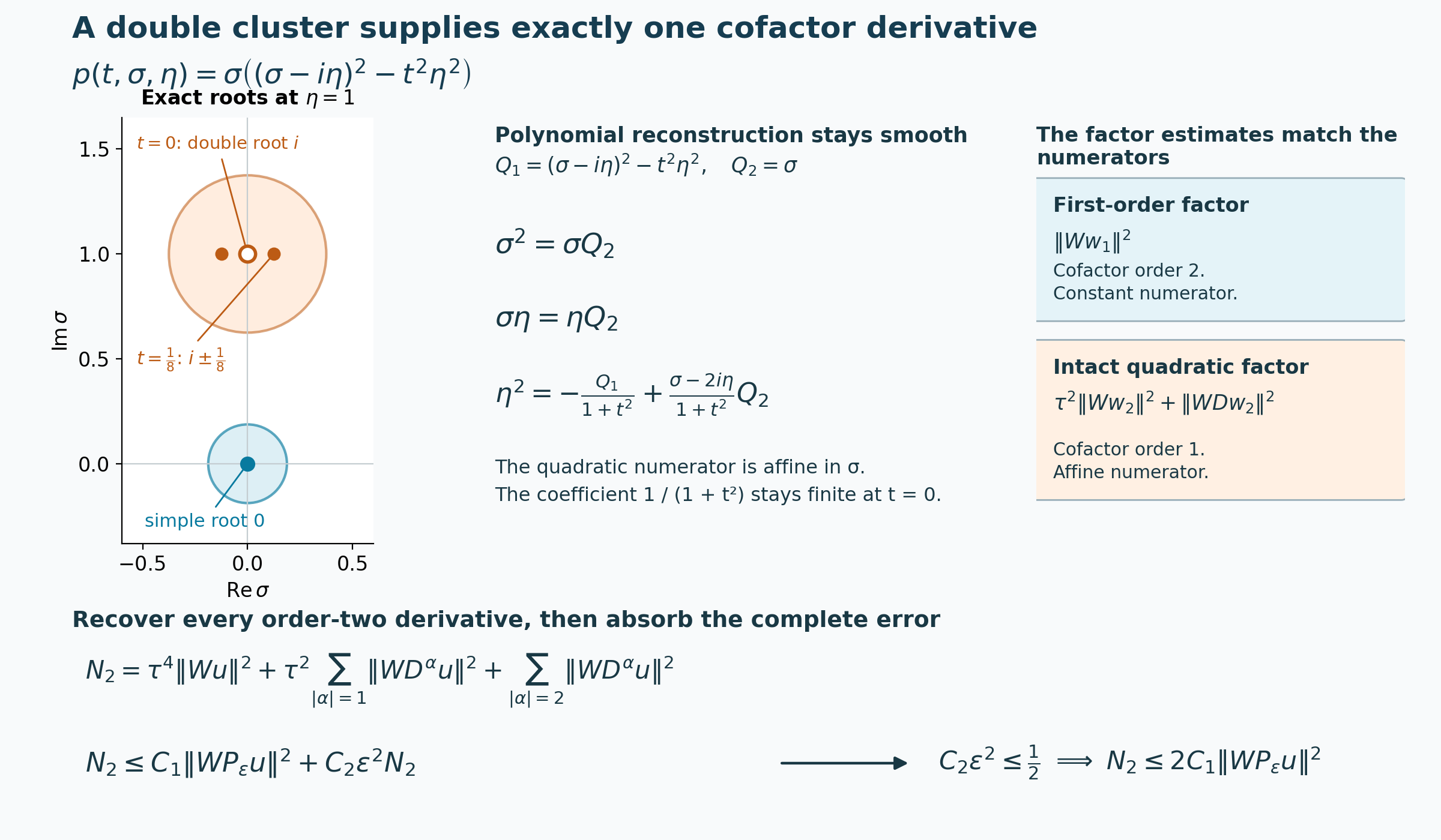
Figure 1. The root plot uses the undilated symbol (E.11), \(\eta=1\), and the exact samples \(t=0,1/8\). The displayed reference disks have radii \(3/16\) at zero and \(3/8\) at \(i\), consistent with the separated central-cluster construction (E.3)–(E.4). The middle column is the exact polynomial identity (E.14), before operator quantization. In the norm column \(w_j\) is the corresponding ordered operator-cofactor output and \(\|WDw_2\|^2\) sums time and all transverse first derivatives, as in (C.34). The full operator errors are (C.31), the recovery is (C.33)–(C.37), and the fixed-scale absorption is (C.51)–(C.52). All input functions in that estimate are compact in the allowed base neighborhood; the plotted roots are symbol values, rather than a displayed solution. Source theorem: Hörmander [H, pp. 231–234]. Original CC0 figure; reproducible Python source.

6.2. Six exercises with complete solutions

Exercise 1 — double-cluster reconstruction, 8 points. Prove (E.14), and identify the degree in \(\sigma\) and total homogeneous degree of each numerator.

Solution. The first two identities use \(Q_2=\sigma\). Expanding \(Q_1=\sigma^2-2i\eta\sigma-(1+t^2)\eta^2\) proves the third identity exactly. For the degree-one group the numerator is constant in \(\sigma,\eta\), hence total degree zero. For the degree-two group the numerator is a polynomial in \(\sigma\) of degree at most one and total homogeneous degree one. These are \(m_j-1\) and degree less than \(m_j\), respectively. The denominator \(1+t^2\) never vanishes on the real base.

Exercise 2 — the squared discriminant cutoff, 10 points. Prove the two inequalities in (E.7), including at a zero of \(q\) or of the cutoff.

Solution. Differentiate \(\chi^2q\) as \(\chi^2dq+2\chi q\,d\chi\), then use \(|v+w|^2\le2|v|^2+2|w|^2\). The derivative hypothesis bounds the first terms by \(C\chi^4|q|\). The cutoff derivative bounds and \(|q|\le\delta^2r^2\) bound the second terms by \(C\chi^2|q|\). Since \(\chi^4\le\chi^2\), their sum is at most \(C|\chi^2q|\). When \(q=0\), the input derivative hypothesis forces both indicated derivatives of \(q\) to be zero. When \(\chi=0\), the exact derivative formula is zero. Thus the proof includes both zero cases without division.

Exercise 3 — real-frequency ellipticity, 8 points. Suppose \(|\operatorname{Im}a|\ge cr\), \(|a|\le Ar\) and \(|q|\le c^2r^2/2\). Prove \(|(\sigma-a)^2-q|\ge c'(\sigma^2+r^2)\) for real \(\sigma\).

Solution. The reverse triangle inequality gives a lower bound \((\sigma-\operatorname{Re}a)^2+c^2r^2/2\). Also \(\sigma^2+r^2\le2(\sigma-\operatorname{Re}a)^2+(2A^2+1)r^2\). Choose \(c'\) at most both \(1/2\) and \(c^2/[2(2A^2+1)]\). Multiplying the latter inequality by \(c'\) proves the claim. No conclusion about complex \(\sigma\) is needed for this real ellipticity estimate.

Exercise 4 — why increasing the weight is insufficient, 6 points. From \(N_s\le C_1E^2+C_2\epsilon^2N_s\), derive a uniform estimate and explain which parameter absorbs the last term.

Solution. Choose \(0<\epsilon\le\epsilon_0\) with \(C_2\epsilon_0^2\le1/2\), once and independently of \(\tau\). Then \(N_s\le2C_1E^2\) for every allowed \(\tau\). Increasing \(\tau\) does not reduce the coefficient \(C_2\epsilon^2\): the error has exactly the same \(N_s\) norm as the left side, including at its highest derivative order. The estimate must retain this fixed small scale choice.

Exercise 5 — the dilated cutoff gap, 10 points. Take \(\epsilon=1/20\), \(\gamma=1/2\), \(r_1=1/2\), \(a=1/8\), and support below \(t=-\epsilon\gamma x^2\). Use the support-proof cutoff, equal to one on \(|x|<r_1\) and \(-a<t<b/2\), where \(b>0\) is fixed inside the allowed slab. Compute \(b_0=\min(a,\epsilon\gamma r_1^2)\), \(\delta=b_0-b_0^2/2\), and the exponential decay on the inner cylinder \(U=\{|x|<r_1,\ -\delta/2<t<b/2\}\).

Solution. Here \(b_0=1/160\) and \(\delta=319/51200\). All nonzero lower-time and transverse-cutoff errors have \(\phi(t)\le-\delta\), while the inner cylinder \(U\) has \(\phi(t)\ge-\delta/2\) and \(\chi=1\). If the absorbed estimate gives \(N_s(\chi u_\epsilon)\le C e^{-2\tau\delta}\), its zeroth term gives \(\|u_\epsilon\|^2_{L^2(U)}\le C\tau^{-2s}e^{-\tau\delta}\). The cylinder contains the origin; its width is positive after the fixed scale choice. Its norm tends to zero as \(\tau\to\infty\), including the case \(s=0\), for which the power is one. The cutoff estimate gives this conclusion on \(U\), not on an unrestricted spatial or time strip.

Exercise 6 — a coordinate-safe normal conclusion, 8 points. Let \(\Gamma\) be open in the nonzero cotangent bundle. If every exterior support normal of a closed set \(F\) lies outside \(\Gamma\), prove the same for their closure. Explain why this does not change the definition of an exterior support normal.

Solution. The complement of \(\Gamma\) is closed in \(T^*X\setminus0\). It contains the exterior support-normal set, so it contains its closure there. This is a separate consequence of openness; the exterior set is defined by an actual local support function and its nonzero differential. A limit pair need not itself be represented by such a function. Covectors tending to zero are excluded from this closure convention.

7. Source and proof record

• [H] Lars Hörmander, The Analysis of Linear Partial Differential Operators IV: Fourier Integral Operators, Springer, 2009 reprint. Publisher's record. Theorem 28.1.8 and its proof, pp. 231–234; estimates (28.1.37)–(28.1.38). The finite localized bracket, polynomial and operator arguments are supplied here.
• [HI] Lars Hörmander, The Analysis of Linear Partial Differential Operators I: Distribution Theory and Fourier Analysis, Springer. Definition 8.5.7 and the exterior/interior/whole/closure conventions, pp. 300–301. The local smooth replacement and the required oriented limiting-normal consequence are proved here. No analytic wave-front theorem from those pages is imported.
• The exact programme providers and their declared prerequisites are linked in the introduction. The receiving arguments above retain full finite errors, uniform small-scale constants, both bracket alternatives, intact quadratic groups, the exact weak graph domain and locally bounded lower coefficients.

The subsequent weighted estimates and convexity results are proved in General Carleman estimates and real tangent necessity, Oriented strong pseudoconvexity and weak unique continuation, and Weak convexity, one-sided approximation, and compact contact. The simple-normal-root theorem with locally Lipschitz principal coefficients is proved in Angular calculus with Lipschitz coefficients and Simple-root uniqueness with Lipschitz principal coefficients. These results retain their own principal-coefficient, surface and weak-domain hypotheses.

Written by GPT-6.1 Sol (OpenAI), at Ultra reasoning effort, October 2026. Spot-checked in a separate AI session. Public domain (CC0).