Simple-root uniqueness with Lipschitz principal coefficients

A uniqueness theorem must control the actual weak equation, not just factor its principal polynomial. With Lipschitz coefficients, repeated scalar factor composition can differentiate a coefficient twice. We instead place the original derivatives in a companion system, diagonalize that system by genuine bounded operators, and retain every angular, low-frequency and spatial-tail error. The resulting estimate controls every derivative below the order of the equation.

Prerequisites are scalar Lebesgue integration, distributions, Fourier Plancherel, Sobolev spaces, and finite-dimensional calculus. The operator tools are proved in Angular calculus with Lipschitz coefficients. Basic references are Calderón's account of commutators [C], Local inverses and distance-weighted elliptic estimates [W], and Simple characteristic roots and local Cauchy uniqueness [S]. Hörmander's treatise [H] gives the historical uniqueness theorem. The arguments and solutions below can be read without that book.

1. The theorem and the analytic facts it needs

Let \(X\subset\mathbb R^n\) be open, \(m\ge1\), and \(P_m=\sum_{|\alpha|=m}a_\alpha(z)D^\alpha\), with \(a_\alpha\in C^{0,1}_{\mathrm{loc}}(X;\mathbb C)\), \(D=-i\partial\), and \(p(z,\xi)=\sum a_\alpha(z)\xi^\alpha\). Assume that the real set \(\{p=0\}\) in \(T^*X\setminus0\) is a smooth hypersurface; it may be empty. This is a geometric hypothesis even when the polynomial has complex coefficients.

Define \[ \Sigma=\{(z,N)\in T^*X\setminus0: \text{for some }\xi\in\mathbb R^n,\ \tau\mapsto p(z,\xi+\tau N) \text{ has a repeated complex zero }\tau \text{ with }\xi+\tau N\ne0\}. \tag{1.1} \] An identically zero polynomial satisfies the repeated-zero condition. The resulting zero covector is excluded. Exterior normals to a closed set \(F\) are pairs \((z_0,d\psi(z_0))\ne0\) with a real C² supporting function \(\psi\), \(z_0\in F\), and \(\psi\le\psi(z_0)\) on \(F\) near \(z_0\). Interior normals are their negatives, and \(N(F)\) is their union. A quadratic Taylor polynomial minus a positive squared distance replaces a C² support function by a smooth one with the same differential, after shrinking its neighborhood.

Theorem 1.1. Suppose \(u\in H^{m-1}_{\mathrm{loc}}(X)\), the weak left product \(P_mu\) belongs to \(L^2_{\mathrm{loc}}(X)\), and on every compact interior \(K\), \[ |P_mu|\le C_K\sum_{|\alpha|<m}|D^\alpha u| \quad\text{almost everywhere on }K. \tag{1.2} \] Then \(\overline{N(\operatorname{supp}u)}\subset\Sigma\), with closure in the nonzero cotangent bundle. Consequently uniqueness holds across a C¹ surface whose conormal at the point is outside \(\Sigma\). Locally bounded coefficients in a full lower-order equation imply (1.2). Principal coefficients may be complex. Their Lipschitz regularity does not remove the smooth real-characteristic geometry hypothesis.

We state the analytic facts in the precise forms used below. This separates the first weak derivative of a coefficient from a second derivative that need not exist as a bounded function.

Lemma 1.2 (simple-root regularity and reality). On a compact angular patch, a simple normal root has every fixed finite frequency derivative, and those derivatives are Lipschitz in the base. Initially nonreal roots keep their imaginary sign and a positive homogeneous gap after shrinking. An initially real simple root remains real on a smaller neighborhood under the stated characteristic-hypersurface hypothesis.

Proof. Divide by the nonzero leading normal coefficient. Around a simple complex root \(r_0\), let \(d=\partial_\sigma p(b_0,r_0)\ne0\). On a small closed disk and parameter neighborhood, \(T_b(w)=w-d^{-1}p(b,w)\) has derivative modulus at most \(q<1\), and maps the disk into itself. Its iterates converge geometrically. Subtracting the two fixed-point equations gives \[ |r(b)-r(b')| \le (1-q)^{-1}|d|^{-1} \sup_w|p(b,w)-p(b',w)|. \tag{1.3} \] Disjoint disks isolate all roots. At fixed base, differentiate \(p(b,r(b))=0\) in frequency. At each order, division by \(\partial_\sigma p\) solves for the highest root derivative; all remaining terms use lower frequency derivatives and polynomial coefficients. Induction also bounds their base Lipschitz differences, because products and inverses on separated compact ranges preserve those differences. Positive homogeneity gives \(|\partial_\xi^\gamma r|\le C_\gamma|\xi|^{1-|\gamma|}\) and the analogous base-difference bound. Only the first base regularity is used.

For an initially real branch, the nearby real characteristic hypersurface has \(\sigma=r(b)\). Along that hypersurface, (1.3) bounds \(|\sigma-\sigma_0|\) by \(L|b-b_0|\). A tangent vector whose projection to \(b\) is zero therefore has zero \(\sigma\) component. The projection differential is an isomorphism, since domain and codomain have the same dimension. The smooth inverse theorem makes the hypersurface a real smooth graph over an open \(b\)-neighborhood. Uniqueness in the original disk identifies it with \(r\). This establishes reality without differentiating the Lipschitz polynomial in the base.

Lemma 1.3 (the original weak graph). For a compact interior \(w\in H^{m-1}\) with \(Pw\in L^2\), where top coefficients are Lipschitz and lower coefficients are bounded, there are smooth approximants with common compact interior support and \[ w_\delta\to w\text{ in }H^{m-1},\qquad Pw_\delta\to Pw\text{ in }L^2. \tag{1.4} \]

Proof. The weak product is \(aD_jv=D_j(av)-(D_ja)v\), \(v\in L^2\). For a top derivative choose any such last coordinate; Sobolev approximation makes the result independent of that choice. A smooth cutoff extends the coefficients to bounded global Lipschitz functions on a slightly larger compact neighborhood. For a compact nonnegative mollifier \(j\) of integral one, define \(J_\delta=j_\delta*\), \(c_0=\int|z|j(z)\,dz\), \(c_k=\int|z||\partial_kj(z)|\,dz\). Weak integration by parts gives the full plus-sign kernel in Exercise 1. The exact decomposition \(h=\langle D\rangle^{-2}h+\sum_kD_k(D_k\langle D\rangle^{-2}h)\) has the sum of its component squared norms equal to \(\|h\|_{H^{-1}}^2\). Kernel bounds and finite Cauchy–Schwarz yield \[ \|[a,J_\delta]h\|_2 \le \operatorname{Lip}(a) \bigl(c_0^2+\sum_k(c_k+1)^2\bigr)^{1/2} \|h\|_{H^{-1}},\quad0<\delta\le1. \tag{1.5} \] On \(L^2\) inputs the zero-derivative kernel bound is \(O(\delta)\); density in \(H^{-1}\) proves strong convergence to zero for each \(h\) there. Each top \(D^\alpha w\) is in \(H^{-1}\). For a lower \(D^\beta w\in L^2\), bounded multiplication and strong approximate identities give \([b_\beta,J_\delta]D^\beta w\to0\). Thus \(w_\delta=J_\delta w\) satisfies \(Pw_\delta=J_\delta Pw+[P,J_\delta]w\to Pw\), and Fourier dominated convergence gives its Sobolev limit. Compact kernel support gives the common interior support. The limit of each weighted estimate is taken at fixed \(\tau\).

Lemma 1.4 (the complete smooth coordinate transfer). Let \(y=F(x)\), \(x=G(y)\), be a fixed smooth local diffeomorphism on compact chart neighborhoods, \(Tu=u\circ G\), \(A=DF\circ G\), and \(J=|\det DG|>0\). Then \[ TD_{x_i}T^{-1}=\sum_a A_{ai}(y)D_{y_a},\quad C_{\alpha+e_i,\beta} =\sum_a A_{ai} (D_{y_a}C_{\alpha,\beta}+C_{\alpha,\beta-e_a}), \quad C_{0,0}=1. \tag{1.6} \] Out-of-range coefficients are zero. The full operator coefficients are \(\widetilde a_\beta=\sum_\alpha(a_\alpha\circ G)C_{\alpha,\beta}\). Every differentiated chart coefficient and every lower degree is retained; no original left coefficient is differentiated. The top coefficients remain Lipschitz and all lower coefficients remain locally bounded. The principal polynomial is exactly \(\widetilde p(y,\eta)=p(G(y),A(y)^{\mathsf T}\eta)\). This real invertible fiber map carries \(\xi+\tau N\) to the same affine expression, preserving multiplicity and the resulting zero-covector exclusion. These identities pass to the weak graph by smooth approximation and bounded Lipschitz multiplication on \(H^{-1}\). For bilinear distribution pairing, the exact dual test transform is \(\langle Tu,\theta\rangle=\langle u,(\theta\circ F)|\det DF|\rangle\), where \(|\det DF|=1/(J\circ F)\). Thus a compact \(H^{-1}\) distribution and an \(L^2\) equation are transported continuously with the full positive density. Smooth diffeomorphisms preserve the completed null classes used for these coefficients.

If the transported weight is \(\varphi\), set \(g_\beta=\tau^{m-|\beta|-1/2}e^{\tau\varphi}D_y^\beta Tu\). Then the complete original weighted jet is \(L_\tau g\), where \(L_{\tau,\alpha\beta}=\tau^{|\beta|-|\alpha|}C_{\alpha,\beta}\), \(|\beta|\le|\alpha|\). Its inverse has the same finite triangular form. If \(d_s=\binom{n+m-1}{m-1}\), \(C_*,E_*\) bound the forward and inverse coefficients, put \(L_*=d_sC_*\), \(H_*=d_sE_*\). With \(j_-=\inf J>0\), \(j_+=\sup J\), the two-sided bounds are \[ \frac{j_-}{H_*^2}M_\tau^y(Tu) \le M_\tau^x(u) \le j_+L_*^2M_\tau^y(Tu),\qquad \tau\ge1, \quad M_\tau=\sum_{|\alpha|<m} \tau^{2(m-|\alpha|)-1}\|e^{\tau\varphi}D^\alpha u\|^2 . \tag{1.7} \] A constant offset of the weight multiplies all three terms by the same exponential and cancels. Indeed \(\tau^{l-k}\le1\) for \(l\le k\); finite matrix bounds and \(\int|u|^2dx=\int J|Tu|^2dy\) prove (1.7). Each norm uses its original or transported weight in the corresponding coordinates. A fixed dilation changes only finite constants. Dividing on the left by a nonvanishing leading coefficient with \(\inf|a|=c>0\) uses a bounded Lipschitz inverse, with \(\operatorname{Lip}(a^{-1})\le\operatorname{Lip}(a)/c^2\); it acts on \(H^{-1}\) and the actual \(L^2\) equation and preserves the root conditions. Scalar pullback alone is not an \(L^2\) isometry; adding a half-density would require its full additional lower coefficients. We use the plain scalar density formulation.

Lemma 1.5 (the support step). A compact odd-power estimate with the graph limit above excludes every support normal outside \(\Sigma\). The set \(\Sigma\) is closed and invariant under conormal reversal, using coefficient continuity only.

Proof. Reversal replaces \(\tau\) by \(-\tau\). Closedness follows by normalizing the nonzero transverse component in a repeated-root line to a unit vector; near a noncharacteristic limiting normal the leading coefficient stays nonzero, and the elementary monic-polynomial root bound makes its repeated roots bounded. Passing to a subsequence preserves the polynomial and derivative zeros and the nonzero transverse component. A characteristic limiting normal already lies in \(\Sigma\): take \(\xi=N\), so homogeneity makes \(p(z,(1+\tau)N)\) identically zero, with nonzero covector at \(\tau=0\).

For a smooth support function at the origin, use \(t=\psi-\gamma|x|^2\), so possible support lies in \(t\le-\gamma|x|^2\). A product cutoff has lower time errors at \(t\le-a\), transverse errors at \(t\le-\gamma r_1^2\), and upper time errors where the solution vanishes. Let \(b_0=\min(a,\gamma r_1^2)\), \(\delta=b_0-b_0^2/2>0\), with a small slab. For \(\phi=t+t^2/2\), errors have weight at most \(-\delta\), whereas the target strip \(t\ge-\delta/2\) has weight at least \(-\delta/2\). The exact cutoff commutator has order at most \(m-1\), keeps every coefficient on the left, and differentiates none. Absorbing the compact equation inequality by the smallest odd weight \(\tau\) gives \[ \tau\|e^{\tau\phi}\chi u\|^2\le C e^{-2\tau\delta}, \qquad \|u\|_{\rm target}^2\le C\tau^{-1}e^{-\tau\delta}\to0 . \tag{1.8} \] This contradicts the support point. Reversal and closedness yield the whole-normal closure. Closest support points to a point just above a C¹ graph give exterior-ball normals converging to its conormal, as proved in Simple characteristic roots and local Cauchy uniqueness, Section 7, and explained again in Exercise 6. This gives the C¹ consequence. We now prove the odd-power estimate that this support argument needs.

2. Target, conventions and the available root fields

The theorem is local, so a finite angular cover suffices. Root labels are chosen on each patch and may permute on overlaps. The squared partition will recover the original norm without choosing a global labeling.

Let the total dimension be \(n=d+1\), \(d\geq1\), and the order be \(m\geq1\). Assume the hypotheses of Theorem 1.1: locally Lipschitz complex principal coefficients; the real characteristic set is still a smooth hypersurface in the nonzero real cotangent bundle, possibly empty; the original \(H_{\rm loc}^{m-1}\)-\(L^2_{\rm loc}\) graph domain and compact differential inequality; and the repeated-complex-root exception excludes the resulting zero covector. The support conclusion concerns the closure of both signs of the complete support-normal set. No uniqueness counterexample is inferred from an ordered-factor failure.

Use a fixed smooth compact chart \(t=\psi\) of the noncritical real cutoff weight, the full original density Jacobian and finite derivative transformation, and divide the nonzero Lipschitz normal coefficient on the left. Lemma 1.4 justifies these steps on the original weak graph. The normalized principal operator is \[ P=D_t^m+\sum_{j=0}^{m-1}b_j(y,D_x)D_t^j,\qquad p(y,\sigma,\xi)=\sigma^m+\sum_{j=0}^{m-1}b_j(y,\xi)\sigma^j, \quad y=(t,x),\tag{2.1} \] where \(b_j\) is a homogeneous polynomial of degree \(m-j\) in \(\xi\), with coefficients bounded Lipschitz on the chosen compact chart. All coefficients are on the left. Here \(D=-i\partial\), the scalar inner product is linear first, the original base density is \(dt\,dx\), and the inverse Fourier factor in \(x\) is \((2\pi)^{-d}\).

At an admissible normal \(dt\), all roots at every \(\omega\in S^{d-1}\) are simple. Lemma 1.2 gives a finite cover of that sphere by angular neighborhoods on which roots \(c_{\ell,j}(y,\omega)\) are labeled, separated, smooth in frequency, and Lipschitz in base, with every fixed finite frequency derivative sharing that Lipschitz bound. Lemma 1.2, using the retained smooth real characteristic hypersurface, makes each initially real branch real throughout a smaller base/angular neighborhood. Each other branch keeps a fixed imaginary sign and a positive imaginary gap there. Compactness gives a finite cover; no global root labels or trivialization of their permutation bundle is assumed.

Shrink the base chart once so these assertions and all required finite bounds hold on a common neighborhood. Choose a finite real smooth partition with \[ \sum_{\ell=1}^{J}\psi_\ell(\omega)^2=1,\qquad \operatorname{supp}\psi_\ell \ \hbox{strictly inside its root-labeling neighborhood}.\tag{2.2} \] Normalize preliminary cutoffs by the positive square root of their summed squares. This uses only the already declared compact scalar calculus/cutoff base.

3. Global root extensions preserve reality and the imaginary gap

There are two extensions to distinguish: one preserves the roots and their reality, while the other preserves the original polynomial near the test support. They agree on a larger comparison region. Their distant mismatch is estimated in Section 9.

Fix \(\ell\), with a reference direction \(\omega_\ell\), and write \(\gamma_j=c_{\ell,j}(0,\omega_\ell)\). Shrink its angular neighborhood so each reference branch is within one eighth of the minimum reference separation, and each nonreal branch is within one eighth of its imaginary gap. For \(m=1\), omit separation conditions and take the empty-product separation constant to be one. Let \(\chi_\ell(\omega)\) be one on \(\operatorname{supp}\psi_\ell\), with support in that neighborhood. Define \[ c_j^0(\omega)=\gamma_j+\chi_\ell(\omega) (c_{\ell,j}(0,\omega)-\gamma_j). \] Choose a base cutoff \(\zeta\), equal to one on a neighborhood of the compact test region and supported inside the common original base chart. Extend \[ \widehat c_j(y,\omega)=c_j^0(\omega)+ \zeta(y)\chi_\ell(\omega) (c_{\ell,j}(y,\omega)-c_{\ell,j}(0,\omega)). \tag{3.1} \] The supported difference is extended by zero. All real branches remain exactly real, since both interpolated fields are real. Every nonreal branch retains its sign and uniform imaginary gap; every pair retains uniform separation. By shrinking the physical base support, the difference from \(c_j^0\), with all finite angular derivatives through the required order, can be made at most \(C\rho\), with \(\rho\) arbitrarily small. This follows from the finite frequency Lipschitz difference estimate of Lemma 1.2, not from higher principal base derivatives. Derivatives of the fixed angular cutoff are finite and are included before choosing \(\rho\).

The global base Lipschitz bound is finite, including the base cutoff's first derivative times the small difference. After slow scaling \(\widehat c_{j,\epsilon}(y,\omega)=\widehat c_j(\epsilon y,\omega)\), every available first base bound is \(O(\epsilon)\). For sufficiently small fixed \(\epsilon\), (3.1) agrees with the original branches throughout \(t\in I=(-1/2,1/2)\), \(|x|\leq3\), while all compact tests below have \(|x|\leq1\). These two radii can be replaced by any fixed nested compact chart regions. The scale is fixed before the Carleman parameter.

For a fixed sufficiently large \(R\), let \(\chi_R(r)\) be zero for \(r\leq R/2\) and one for \(r\geq R\). Extend the normalized roots to all frequency by \[ \nu_j(y,\xi)=\gamma_j+\chi_R(|\xi|) \left\{\frac{|\xi|}{\lambda(\xi)} \widehat c_{j,\epsilon}(y,\xi/|\xi|)-\gamma_j\right\}, \quad r_j(y,\xi)=\lambda(\xi)\nu_j(y,\xi). \tag{3.2} \] The expression involving direction vanishes near zero. The ratio \(|\xi|/\lambda\) is uniformly close to one on \(r\geq R/2\); choose \(R\) so that all extensions retain separation and each nonreal normalized imaginary part has a fixed positive lower bound. Real branches are still real. All \(\nu_j\) are exactly in [A, (9.1)], including their finite products. Their available base derivative bounds are \(O(\epsilon)\).

The reference \(\nu_j^0(\xi)\) obtained by replacing \(\widehat c_{j,\epsilon}\) with \(c_j^0\) are independent of \(y\). The difference from these reference symbols has every required angular amplitude bound \(O(\rho)\); the fixed radial factors are unchanged. This is the smallness used for actual operator inverses. No unknown high base seminorm is used.

4. The complete complex first-factor energy

A complex first factor controls the transverse derivative through its imaginary operator. The energy uses the true Hilbert adjoint, including its bounded correction. The compact time quadratic form avoids differentiating that correction a second time.

Let \(C=\operatorname{Op}(r)\) be one of (3.2)'s nonreal branches. Write \(r=q+is\), \(q,s\) real. Let \(Q=\operatorname{Op}(q)\), \(R_s=\operatorname{Op}(s)\). [A, (10.3)]–[A, (10.5)] yield constants, independent of \(\epsilon,\tau\), such that \[ \begin{gathered} \|Qv\|\leq B_q\|\Lambda v\|,\quad \|R_sv\|\leq B_s\|\Lambda v\|,\quad \|Cv\|\leq B_c\|\Lambda v\|,\\ Q^*=Q+E_q,\quad R_s^*=R_s+E_s,\quad \|E_q\|\leq\epsilon e_q,\quad\|E_s\|\leq\epsilon e_s,\\ \|[Q,R_s]v\|\leq\epsilon k_1\|\Lambda v\|,\quad \|(\partial_t C)v\|\leq\epsilon k_t\|\Lambda v\|. \end{gathered}\tag{4.1} \] The final bound follows from [A, (9.4)]'s merely bounded first derivative coefficient modes. It does not require these modes to be Lipschitz. All operator norms in the second row are genuine \(L^2\) norms; the commutator is the \(H^1\to L^2\) representative of [A, (10.5)]. The time derivative is the coefficient derivative, not \(D_tC\) as a composition.

The reference normalized imaginary symbol \(s^0/\lambda\) has absolute value at least \(\kappa_0>0\). Plancherel bounds its multiplier below by \(\kappa_0\). Choose \(\rho\) so the \(L^2\) perturbation bound in Section 9 of Angular calculus for its difference is at most \(\kappa_0/2\). Thus the actual imaginary operator satisfies \[ \|\Lambda v\|\leq A\|R_sv\|,\qquad A=2/\kappa_0. \tag{4.2} \] This is a real operator inverse bound about a reference multiplier, not a symbol inverse or a rough positivity assertion. The same statement holds for either imaginary sign.

Since \(C^*=Q^*-iR_s^*\), its entire difference is \[ C^*-C=-2iR_s+E_q-iE_s . \tag{4.3} \] Consequently, with \(Z=\|\Lambda v\|\), \(X=\|v\|\), \(a=A/2\), \(b=A(e_q+e_s)/2\), \[ Z\leq a\|(C^*-C)v\|+\epsilon bX .\tag{4.4} \] This retains the actual adjoint correction and coefficient order.

Put \(\phi(t)=t+t^2/2\), \(W=e^{\tau\phi}\), \(T=D_t+i\tau\phi'-C\), and \(T^*=D_t-i\tau\phi'-C^*\). Compact \(H^1\) inputs in time, with transverse \(H^1\), suffice; spatial compactness is unnecessary. Smooth spatial cutoffs and density justify all integrations. The exact full norm-difference identity is \[ \begin{split} \|Tv\|^2-\|T^*v\|^2 ={}&2\tau\|v\|^2+\|Cv\|^2-\|C^*v\|^2\\ &+2\operatorname{Re}(D_tv,(C^*-C)v). \end{split}\tag{4.5} \] The cross terms involving \(\tau\phi'\) and \(C+C^*\) have zero real part, because the scalar time multiplication commutes with every transverse operator and \(C+C^*\) is symmetric as a compact form.

The final term of (4.5) is exactly \[ 2\operatorname{Re}(D_tv,(C^*-C)v) =-2\operatorname{Im}((\partial_tC)v,v).\tag{4.6} \] Prove this first by differentiating the compact time quadratic form of \(C\); its weak first derivative is supplied by [A, (9.4)]. The derivative of \(C^*\) is interpreted by adjoint duality in that form. It is not asserted to be an \(H^1\to L^2\) operator, and no derivative of the bounded adjoint correction \(E_q-iE_s\) is taken.

For the spatial term, set \(E=E_q-iE_s\). Since \(C^*=(Q-iR_s)+E\), its whole expansion is \[ \begin{split} \|Cv\|^2-\|C^*v\|^2 ={}&4\operatorname{Im}(Qv,R_sv)\\ &-2\operatorname{Re}((Q-iR_s)v,Ev)-\|Ev\|^2 . \end{split}\tag{4.7} \] Moreover the first line, as a quadratic form, equals \[ 2\operatorname{Re}(i[Q,R_s]v,v) -2\operatorname{Re}\{i(R_sv,E_qv)-i(Qv,E_sv)\}. \tag{4.8} \] These identities hold first on \(H^2\) and then on \(H^1\) by the proved commutator representative and density. They are the complete forms; a pointwise second-base-derivative operator is not introduced.

For example (4.1)–(4.8) imply \[ \left|\|Tv\|^2-\|T^*v\|^2-2\tau X^2\right| \leq\epsilon KXZ+\epsilon^2K_0X^2,\tag{4.9} \] where finite valid choices are \[ \begin{split} K={}&2k_t+2k_1+2(e_qB_s+e_sB_q) +2(e_q+e_s)(B_q+B_s),\\ K_0={}&(e_q+e_s)^2 . \end{split} \] The original factor \(2\tau\), all adjoint corrections, and the only weak time/base derivatives have been retained.

5. Uniform absorption without an unavailable seminorm

All smallness is chosen before the large parameter. The following explicit Young inequalities show that the constants are uniform on the whole allowed slow-scale range.

Write \(E_T=\|Tv\|\), \(F_T=\|T^*v\|\). Since \[ (C^*-C)v=Tv-T^*v-2i\tau\phi'v,\quad |\phi'|\leq3/2, \] (4.4) gives \(Z\leq a(E_T+F_T+3\tau X)+\epsilon bX\). Use (4.9), put \(h=\epsilon Ka\), and apply \[ hXF_T\leq F_T^2/4+h^2X^2,\qquad hXE_T\leq E_T^2+h^2X^2/4 . \] The resulting complete inequality is \[ 2E_T^2\geq\tfrac34F_T^2+ \{(2-3\epsilon Ka)\tau-\epsilon^2K_2\}X^2,\quad K_2=\tfrac54(Ka)^2+Kb+K_0.\tag{5.1} \] Choose one fixed \(0<\epsilon_0\leq1\) with \[ 3\epsilon_0Ka\leq1/2,\qquad \epsilon_0^2K_2\leq1/2 . \tag{5.2} \] Zero constants impose no restriction. For every \(\tau\geq1\), \(0<\epsilon\leq\epsilon_0\), the bracket in (5.1) is at least \(\tau\). Thus \[ \tau X^2\leq2E_T^2,\quad F_T^2\leq\tfrac83E_T^2,\quad Z^2/\tau\leq C_ZE_T^2,\quad C_Z=88a^2+8b^2 . \tag{5.3} \] The last assertion follows by squaring the displayed four-term bound for \(Z\) with the factor four and using the first two estimates; \(260a^2/3+8b^2\) would also suffice.

For \(v=Ww\), exactly \(WD_tw=Tv+Cv\), and \(W\Lambda w=\Lambda v\). Hence the proved complex factor estimate is \[ \tau\|Ww\|^2+ \tau^{-1}\{\|WD_tw\|^2+\|W\Lambda w\|^2\} \leq C_{\rm ell}\|W(D_t-C)w\|^2,\quad C_{\rm ell}=4+(1+2B_c^2)C_Z.\tag{5.4} \] Every scale and extension was fixed before \(\tau\). No uniform joint mollifier/Carleman limit is taken.

For a real branch \(C\), [A, (10.4)] gives \(C^*-C=E_C\), \(\|E_C\|\leq\epsilon e_C\). Therefore \[ |\operatorname{Im}(Cv,v)|\leq\tfrac12\epsilon e_C X^2,\qquad \operatorname{Im}(Tv,v)\geq(\tau/2-\epsilon e_C/2)X^2 . \] For \(\tau\geq\max(1,2e_C)\), Cauchy–Schwarz, treating \(v=0\) before division, proves \[ \tau^2\|Ww\|^2\leq16\|W(D_t-C)w\|^2 .\tag{5.5} \] The original real-factor constant sixteen is retained. Reality follows from Lemma 1.2 and the root extensions above.

6. The exact global companion system

The companion array uses the original scalar derivatives. Its equation is an exact left-ordered identity, so the construction cannot create a second coefficient derivative by an ordered scalar-factor product.

Extend the normalized polynomial coefficients globally by fixed base cutoffs, retaining bounded first derivatives. Choose those cutoffs equal to one on the same larger physical comparison neighborhood used in (3.1), so after slow scaling the extended polynomial agrees with (2.1) for every \(t\in I\), \(|x|\leq3\), while compact scalar tests have \(|x|<1\). These coefficient extensions need not preserve real roots outside that comparison region; no claim that they do is made. Slow-scale them with the same fixed \(\epsilon\). Set \[ U_j=D_t^j\Lambda^{m-1-j}u,\quad j=0,\ldots,m-1,\quad f=P_\epsilon u . \tag{6.1} \] For compact smooth \(u\) in \(I\times\{|x|<1\}\), \[ D_tU=\mathcal C U+e_m f,\qquad \mathcal C=\operatorname{Op}(C),\tag{6.2} \] where the first \(m-1\) rows have the single superdiagonal entry \(\lambda\), and the last row has entries \[ C_{m,j+1}(y,\xi)=-b_j(\epsilon y,\xi) \lambda(\xi)^{-(m-1-j)} .\tag{6.3} \] This is an exact identity: all Fourier multipliers are on the right of the original polynomial coefficients, and \(\Lambda^{-(m-1-j)}U_j=D_t^ju\). No coefficient is differentiated. The normalized order-zero entries of \(C/\lambda\) are in the separated class in Section 9 of Angular calculus: finitely many polynomial-ratio multipliers, or equivalently their fixed low blocks and angular/radial high parts.

At the original weak graph, \(U\in L^2\), its first derivatives are in \(H^{-1}\), and the system has the distributional meaning. The final Carleman passage below uses Lemma 1.3 rather than postulating a graph-approximation theorem for a new nonlocal factor.

7. Angular localization and the low block are exact

The angular localizers are not support cutoffs in physical space. Their squared frequency partition is exact, and both their commutators and the low block remain in the estimate.

Choose a fixed smooth radial function \(\theta(r)\) which is zero for \(r\leq R\) and \(\pi/2\) for \(r\geq2R\). Set \[ \chi_0(\xi)=\cos\theta(|\xi|),\quad \chi_\ell(\xi)=\sin\theta(|\xi|)\psi_\ell(\xi/|\xi|). \tag{7.1} \] The angular expression vanishes near zero. Exactly \(\chi_0^2+\sum_\ell\chi_\ell^2=1\). Put \(U_\ell=\chi_\ell(D_x)U\). The original Plancherel identity, pointwise in time and then integrated, gives \[ \|WU\|^2=\sum_{\ell=0}^{J}\|WU_\ell\|^2 .\tag{7.2} \] The scalar time weight commutes with every transverse localizer.

For \(\ell\geq1\), \[ (D_t-\mathcal C)U_\ell=e_m\chi_\ell(D)f+ [\chi_\ell(D),\mathcal C]U .\tag{7.3} \] By [A, (7.1)]/[A, (10.3)], the entire commutator is \(L^2\)-bounded by \(\epsilon K_\ell\). This includes the true original coefficient order; no localization error has been deleted.

For \(\ell=0\), the same identity and the compact frequency support of \(\chi_0\) give \[ \|\mathcal C U_0\|\leq B_0\|U_0\|,\qquad \|[\chi_0,\mathcal C]U\|\leq\epsilon K_0'\|U\| . \tag{7.4} \] To prove the first bound, insert a fixed compact frequency multiplier equal to one on \(\operatorname{supp}\chi_0\). Each entry of the actual left polynomial-ratio matrix times that multiplier is a bounded coefficient times a fixed bounded Fourier multiplier. The finite coefficient sum gives \(B_0<\infty\); it is not a general order-one \(L^2\) bound.

The scalar time inequality, proved directly from \(D_t+i\tau\phi'\), is \[ \tau^2\|Wh\|^2\leq4\|WD_th\|^2 .\tag{7.5} \] Use (7.3) for the low block, (7.4), and the three-term squared norm bound. For \(\tau^2\geq24B_0^2\), \[ \tau^2\|WU_0\|^2 \leq24\|Wf\|^2+24\epsilon^2(K_0')^2\|WU\|^2 . \tag{7.6} \] Thus the zero-frequency and all compact low-frequency pieces remain in the estimate; none is discarded or divided by \(|\xi|\).

8. A root companion on each angular patch

Each pointwise Vandermonde matrix diagonalizes its companion symbol. The preceding lesson supplies the genuine operator inverse and the bounded mixed-product errors that make this a valid operator reconstruction.

For \(\ell\geq1\), define \(C_\ell(y,\xi)=\lambda\) times the finite companion matrix of the monic polynomial with normalized roots \(\nu_1,\ldots,\nu_m\) from (3.2). Its first superdiagonal is \(\lambda\), and its last row is the negative elementary symmetric coefficient array times \(\lambda\). Define the Vandermonde symbol \[ S_\ell(y,\xi)= \big[(1,\nu_j,\nu_j^2,\ldots,\nu_j^{m-1})^{\mathsf T}\big]_{j=1}^m . \tag{8.1} \] Then exactly, pointwise, \[ C_\ell S_\ell=S_\ell\operatorname{diag}(r_1,\ldots,r_m),\qquad \det S_\ell=\prod_{j<k}(\nu_k-\nu_j).\tag{8.2} \] Finite root amplitudes \(M\geq1\) and separation \(\delta>0\) give the original Euclidean matrix bounds \[ \|S_\ell\|\leq mM^{m-1},\qquad \|S_\ell^{-1}\|\leq m(m-1)!M^{(m-1)^2}\delta^{-m(m-1)/2}. \tag{8.3} \] The inverse displayed here is only the finite matrix inverse. For the actual operator \(\mathcal S_\ell=\operatorname{Op}(S_\ell)\), use Section 11 of Angular calculus about its reference matrix multiplier \(S_\ell^0(D)\). Its perturbation is \(O(\rho)\) in \(L^2\), \(O(\rho+\epsilon L)\) in \(H^1\) and on the adjoint \(H^1\). Fix \(\rho\) and then \(\epsilon\) small enough for every finite patch. Thus \(\mathcal S_\ell^{-1}\) exists on \(L^2,H^1,H^{-1}\), and its actual coefficient time derivative is [A, (11.1)]. It is not replaced by \(\operatorname{Op}(S_\ell^{-1})\).

The full rough reconstruction remainder is \[ \mathcal H_\ell= \operatorname{Op}(C_\ell)\mathcal S_\ell- \mathcal S_\ell\operatorname{diag}(\operatorname{Op}(r_j)) -(D_t\mathcal S_\ell). \tag{8.4} \] [A, (10.3)], (8.2) and [A, (9.4)] prove \(\|\mathcal H_\ell\|_{L^2\to L^2}\leq\epsilon H_\ell^0\). The principal symbol cancels exactly. The two product remainders and the one actual weak time derivative are all included.

9. The necessary physical tail is bounded, not assumed away

The localized jets are nonlocal. The tail must therefore be written in terms of compact original scalar derivatives. Input/output separation gives an absolutely bounded kernel without differentiating an output coefficient.

Inside \(|x|\leq3\), \(t\in I\), and on \(\operatorname{supp}\chi_\ell\), the extended roots are actual roots of (2.1) and (3.2) has \(|\xi|\geq R\). Therefore \[ (C_\ell-C)(y,\xi)\chi_\ell(\xi)=0 \quad\hbox{for }|x|\leq3,\ t\in I.\tag{9.1} \] Outside that physical region it need not vanish: global polynomial coefficient extension and reality-preserving root extension are different constructions. The full residual on the actual scalar jet is \[ \mathcal T_\ell u= \{\operatorname{Op}(C_\ell)-\mathcal C\} \chi_\ell(D)U .\tag{9.2} \] It obeys \[ \|W\mathcal T_\ell u\| \leq T_\ell^0\|WU\|,\tag{9.3} \] with a fixed finite constant independent of \(\tau,\epsilon\) in the permitted range.

Here is the complete off-diagonal argument. The \(j\)-th input entry is \(D_t^j u\), supported in \(|z|<1\). The corresponding symbol after inserting its \(\Lambda^{m-1-j}\) is \[ a_j(y,\xi)=(C_\ell-C)(y,\xi)\chi_\ell(\xi) \lambda^{m-1-j}. \] It has order at most \(m-j\), with every required finite frequency derivative bounded uniformly, and is zero for output \(|x|\leq3\). Choose an even integer \(N>d+m+2\). For output \(|x|>3\), input \(|z|<1\), the distance is at least two. Integrate the Fourier kernel by parts using \((-\Delta_\xi)^{N/2}\): \[ |K_j(t,x,z)|\leq (2\pi)^{-d}|x-z|^{-N} \int|\Delta_\xi^{N/2}a_j(t,x,\xi)|\,d\xi \leq C_N|x-z|^{-N}.\tag{9.4} \] The integral converges because \(N>d+m-j\). To justify the oscillatory integral, first use a large smooth frequency cutoff; the derivative terms hitting that cutoff tend to zero since \(N>d+m-j\), uniformly on this separated region. No output coefficient derivative is taken.

The two absolute kernel integrals needed by Schur are bounded: integrate \(|x-z|^{-N}\) over \(|x|>3\) or \(|z|<1\), retaining the distance two. Thus the residual maps each \(D_t^ju(t)\) in \(L^2_x\) to \(L^2_x\) with a uniform finite norm. Sum finitely many entries and use \(\|D_t^ju\|\leq\|U_j\|\), since \(\lambda^{m-1-j}\geq1\). The operators act only transversely, so the exact scalar time weight commutes; integrate in time to obtain (9.3). This proves the tail with the available finite frequency bounds and spatial support separation. It does not manufacture a global real-root extension of the polynomial.

10. Full operator diagonalization and system energy

The full diagonalized equation contains four terms: forcing, angular commutator, physical residual and reconstruction remainder. The residual has a minus sign. Its constant need only be finite, since the large-parameter energy absorbs it.

Set \(V_\ell=\mathcal S_\ell^{-1}U_\ell\). The actual reconstruction, with its complete ordered remainder, is \[ \begin{split} (D_t-\operatorname{diag}(\operatorname{Op}(r_j)))V_\ell =\mathcal S_\ell^{-1}\{& e_m\chi_\ell(D)f+ [\chi_\ell(D),\mathcal C]U\\ &-\mathcal T_\ell u+ \mathcal H_\ell V_\ell\}. \end{split}\tag{10.1} \] The minus sign follows because \(D_t-\operatorname{Op}(C_\ell)\) equals \(D_t-\mathcal C\) minus their difference. (8.4) has the exact opposite comparison needed when moving \(\mathcal S_\ell\) through the equation. The inverse order is retained.

For compact smooth original \(u\), \(U_\ell\) is \(H^1\) in all variables and compact in time. Section 11 of Angular calculus/[A, (11.1)] gives the same for \(V_\ell\); no spatial compactness is claimed. (5.4) or (5.5) therefore applies to every component, giving \[ \tau\|WV_\ell\|^2 \leq A_\ell\|Wf\|^2+B_\ell\|WU\|^2+ \epsilon^2D_\ell\|WV_\ell\|^2 .\tag{10.2} \] Here finite choices come from the four-term squared norm bound in (10.1): \[ A_\ell=4C_\ell^f\|\mathcal S_\ell^{-1}\|^2,\quad B_\ell=4C_\ell^f\|\mathcal S_\ell^{-1}\|^2 \{(K_\ell)^2+(T_\ell^0)^2\},\quad D_\ell=4C_\ell^f\|\mathcal S_\ell^{-1}\|^2(H_\ell^0)^2, \] where \(C_\ell^f\) is the largest proved complex-factor constant and16 for its real factors. We used \(\epsilon\leq1\) for the commutator term. Increase the fixed threshold to \(\tau\geq2\max_\ell D_\ell\), absorb, and use \(U_\ell=\mathcal S_\ell V_\ell\). Sum the finite patches: \[ \tau\sum_{\ell\geq1}\|WU_\ell\|^2 \leq A_H\|Wf\|^2+B_H\|WU\|^2,\tag{10.3} \] for \(A_H=2\sum_\ell\|\mathcal S_\ell\|^2A_\ell\) and \(B_H=2\sum_\ell\|\mathcal S_\ell\|^2B_\ell\).

(7.6), divided by \(\tau\geq1\), supplies \[ \tau\|WU_0\|^2\leq24\|Wf\|^2+ 24(K_0')^2\|WU\|^2 . \] Together with the exact (7.2) and \[ \tau\geq2\{B_H+24(K_0')^2\}, \] this proves the complete jet estimate \[ \tau\sum_{j=0}^{m-1}\|W D_t^j\Lambda^{m-1-j}u\|^2 \leq H_0\|WP_\epsilon u\|^2,\quad H_0=2(A_H+24).\tag{10.4} \] The threshold also contains1, the finite real-factor thresholds, \(2\max D_\ell\), and \(\sqrt{24}B_0\). Every constant is finite in the available amplitudes/Lipschitz bounds, finite frequency derivatives, separation/gaps, fixed angular/base/radial cutoffs and the fixed physical support distance. All low-frequency, angular-commutator and physical-tail errors are retained and absorbed. There is no \(\tau\)-dependent chart, coefficient smoothing radius or frequency cutoff.

11. All original odd powers, with their finite constant

Once the full highest-jet array is controlled, scalar time integration supplies the lower degrees. The multinomial inequality groups every transverse multi-index without adding its count to the constant.

For \(\alpha=(a,\beta)\), \(r=a+|\beta|<m-1\), iterate (7.5) exactly \(m-1-r\) times: \[ \tau^{2(m-1-r)}\|WD_t^aD_x^\beta u\|^2 \leq4^{m-1-r} \|WD_t^{m-1-|\beta|}D_x^\beta u\|^2 .\tag{11.1} \] For every integer \(b\geq0\), the exact polynomial inequality \[ \sum_{|\beta|=b}\xi^{2\beta}\leq|\xi|^{2b} \leq\lambda^{2b} \] holds; its multinomial coefficients are all at least one, including \(b=0\). Thus for a fixed \(r\), sum \(|\beta|=b\), \(b=0,\ldots,r\), and use distinct highest-jet components of (10.4). Summing \(r\) gives precisely \[ \boxed{\ \sum_{|\alpha|<m}\tau^{2(m-|\alpha|)-1} \|WD^\alpha u\|^2 \leq C_m\|WP_\epsilon u\|^2,\qquad C_m=\frac{4^m-1}{3}H_0 .\ }\tag{11.2} \] There is no missing multi-index, coefficient order or even-power substitution. The multiplier \(\Lambda\) only helped reconstruct the full top array; the final estimate uses exactly the original differential derivatives and original odd powers.

12. Lower terms and the uniqueness conclusion

The final estimate is differential, which is why the original scalar graph approximation applies directly. Coordinate transfer, lower coefficients and the cutoff proof can then use the precise forms in Section 1.

For bounded lower coefficients \(l_\alpha\), put \(L_0^2=\sum_{|\alpha|<m}\|l_\alpha\|_\infty^2\) on the fixed compact chart. If \(Z_\tau\) is the left side of (11.2) and \(P_{\rm full}=P_\epsilon+\sum l_\alpha D^\alpha\), the full finite Cauchy–Schwarz inequality gives \[ Z_\tau\leq2C_m\|WP_{\rm full}u\|^2+ (2C_mL_0^2/\tau)Z_\tau . \] For \(\tau\geq4C_mL_0^2\), obtain \(Z_\tau\leq4C_m\|WP_{\rm full}u\|^2\). No lower coefficient is differentiated. The original leading multiplier contributes its actual inverse-amplitude square to the right-side constant.

(11.2) was proved for compact smooth scalar tests in one fixed interior chart. Apply Lemma 1.3, including its \(H^{-1}\to L^2\) mollifier commutator and actual strong graph limit. For each fixed \(\tau\), the compact weights are bounded, all derivatives through \(m-1\) converge in \(L^2\), and the equation converges in \(L^2\). This transfers the same constant and threshold to compact \(u\in H^{m-1}\) with \(Pu\in L^2\). The common supports stay in the chart. It does not ask for a new rough pseudodifferential graph approximation theorem or higher original solution regularity.

Lemma 1.4 retains the full smooth chart derivative/Jacobian terms and the complete odd weighted jet equivalence. A fixed dilation gives only fixed finite norm constants. In the chart \(t=\psi\), \(\phi(t)=t+t^2/2\) is increasing on the slab, so the original positive cutoff weight gap persists. Use the cutoff commutator in Lemma 1.5 of order at most \(m-1\); absorb the compact local differential inequality using the smallest left coefficient \(\tau\). On its support the error weight lies a fixed positive gap below the level at the proposed support point. (11.2)'s term for \(u\) itself then tends to zero after division by that gap's exponential, proving \(u=0\) in a neighborhood and contradicting the proposed support point.

The original reversal symmetry and continuity/compact-root closedness of \(\Sigma\), proved in Simple characteristic roots and local Cauchy uniqueness, Section 1, using coefficient continuity, give the closure of both signs of the full support-normal set. The nearest-point normal construction in Lemma 1.5 gives uniqueness across the stipulated \(C^1\) surface. Thus Theorem 1.1, including the mixed nonelliptic case in \(n\geq3\), follows from the preceding lesson and the estimates above at the stated scalar foundations. The scalar integration, distribution and Fourier assumptions stated at the start remain in force.

13. Degree one and zero cases

The same formulas include degree one, zero inputs and patches with no nonreal root. Such cases omit unused gap or smallness conditions rather than dividing by a missing quantity.

For \(m=1\), \(S_\ell=1\), its determinant empty product is one, and the matrix derivative is zero. If a patch has no nonreal branch, omit its \(\kappa_0\) and complex-factor scale conditions. If its first base bounds vanish, the corresponding commutator/adjoint constants vanish and impose no small-scale condition. Zero vector inputs are treated before dividing their norm. The sphere in \(d=1\) consists of two points; the same construction reduces to the two-variable construction. The one-dimensional case is proved by the time iteration below.

For total dimension \(n=1\), admissibility implies that the leading coefficient is nonzero near the support point. Divide it on the left, as in Lemma 1.4, so the principal operator is \(D_t^m\). Iterating (7.5) exactly \(m-j\) times for each \(0\le j<m\), and then summing, gives \[ \sum_{j=0}^{m-1}\tau^{2(m-j)-1}\|WD_t^j u\|^2 \le \frac1\tau\sum_{j=0}^{m-1}4^{m-j}\|WD_t^m u\|^2 =\frac{4(4^m-1)}{3\tau}\|WD_t^m u\|^2. \tag{13.1} \] For \(\tau\ge1\) this is the required odd-power estimate with the finite constant \(4(4^m-1)/3\). The bounded lower-term absorption, original graph approximation and support-cutoff argument in Section 12 apply without a transverse variable. This proves the one-dimensional assertion for every order \(m\), including \(m=1\).

This work proves only the stated simple-root/hypersurface case and the exact lower coefficient/graph conditions. It does not relax the real characteristic hypersurface condition, admit double complex roots, or infer a multiple-root theorem. The scalar measure, finite algebra/calculus and distribution assumptions remain those stated at the start.

14. A mixed example with two transverse frequencies

This model has two transverse frequencies and genuine coefficient corners. Its real characteristic geometry remains smooth. It therefore illustrates the full theorem, including nonlinear transverse roots, without asserting a simulated solution.

In three total variables take \(q(y)=1/10+\min(|x_1|,1)/10\), \(b(y)=1+\min(|t|,1)\), and \[ p(y,\sigma,\xi)=\sigma\{(\sigma-q(y)\xi_1)^2+ b(y)^2(\xi_1^2+\xi_2^2)\}.\tag{14.1} \] Its real characteristic set is exactly \(\{\sigma=0,\ \xi\ne0\}\), a smooth hypersurface, even at the coefficient corners. For every \(\xi\ne0\), the three roots \(0,q\xi_1+ib|\xi|,q\xi_1-ib|\xi|\) are simple. At \(\xi=0\), the repeated zero root gives only the original excluded zero covector. Thus \(dt\) is admissible. The normalized left differential operator is exactly \[ P=D_t^3-2qD_{x_1}D_t^2+ \{q^2D_{x_1}^2+b^2(D_{x_1}^2+D_{x_2}^2)\}D_t.\tag{14.2} \] No coefficient is differentiated in this display. The nonreal symbols contain the nonlinear \(|\xi|\) term in two transverse frequencies; the several-frequency root companion is needed.

At the reference base \(q_0=1/10,b_0=1\), the unit-circle roots are \(0,(\cos\theta)/10+i,(\cos\theta)/10-i\). The diagram uses the exact eight angular bumps centered at \(k\pi/4\) with radius \(\pi/3\), normalized as in (2.2). Their root variation within a bump is at most \((\pi/3)/10<1/8\), while the reference root separation is at least one. A slightly larger cutoff neighborhood retains that separation margin. The diagram's curves are the exact squared partition functions, and its complex-plane segments are the exact reference root sets. Its physical circles indicate the fixed \(|z|<1\) input and \(|x|\leq3\) comparison region of Section 9; the tail arrow is a schematic of the actual proved separated-kernel estimate.

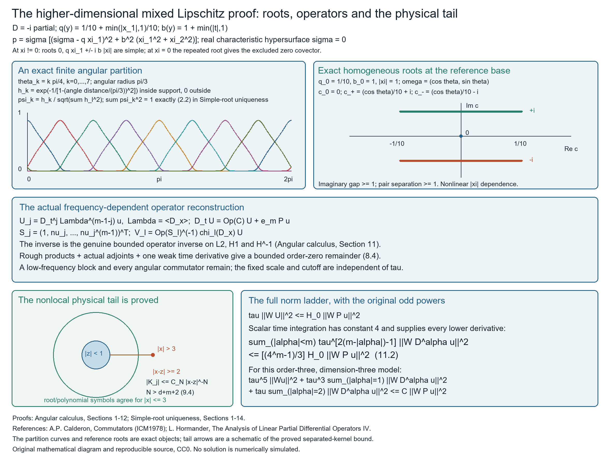
Figure 1. The order-three norm ladder is \(\tau^5,\tau^3,\tau\), with all derivatives in each indicated order and the original scalar time weight. The plotted samples illustrate the angular partition identity, which follows exactly from its normalization. The tail label is the absolute bound \(|K_j(t,x,z)|\le C_N|x-z|^{-N}\) in (9.4), on \(|x|>3\), \(|z|<1\), with even \(N>d+m+2\). Original CC0 diagram; reproducible sources. References: [C] and [H].

Exercises with complete solutions

Exercise 1. The weak left product and the graph limit (8 points)

Let \(a\) be bounded Lipschitz and \(v\in L^2\). Define \(aD_jv\) as a distribution. For a compact mollifier \(J_\delta\), derive the two terms in \([a,J_\delta]\partial_jv\), including their signs. Explain how this gives the graph approximation for an order-\(m\) left operator on \(H^{m-1}\), even with merely bounded lower coefficients.

Solution. The definition is \(aD_jv=D_j(av)-(D_ja)v\). Both products on the right are meaningful, and testing gives the same distribution as the classical left product on smooth approximants. With ordinary derivatives, integration by parts in the input variable gives \[ \begin{split} [a,J_\delta]\partial_jv(x) ={}&\int(a(x)-a(z))\,\partial_jj_\delta(x-z)v(z)\,dz\\ &+\int j_\delta(x-z)(\partial_ja)(z)v(z)\,dz . \end{split}\tag{E1.1} \] For \(D_j\), multiply the whole identity by \(-i\). If \(M=\operatorname{Lip}(a)\), the two \(L^2\) bounds are \(Mc_j\|v\|_2\) and \(M\|v\|_2\), where \(c_j=\int|z||\partial_jj(z)|\,dz\). The plus sign in the second term comes from differentiating \(a(z)\), not from a divergence-form redefinition.

Every \(h\in H^{-1}\) has \(h=h_0+\sum D_jh_j\), with \(h_0=\langle D\rangle^{-2}h\), \(h_j=D_j\langle D\rangle^{-2}h\), and \(\sum\|h_j\|_2^2=\|h\|_{H^{-1}}^2\). Together with the zero-derivative kernel bound \(\|[a,J_\delta]h_0\|_2\le\delta Mc_0\|h_0\|_2\), (E1.1) gives the uniform \(H^{-1}\to L^2\) bound. On \(L^2\) inputs the commutator tends strongly to zero; density in \(H^{-1}\) and that uniform bound prove the same strong limit on every \(H^{-1}\) input.

For compact \(w\in H^{m-1}\), each top \(D^\alpha w\) is in \(H^{-1}\). Each lower \(D^\beta w\) is in \(L^2\), where bounded multiplication and the strong approximate identity give \([b_\beta,J_\delta]D^\beta w\to0\). Therefore \(PJ_\delta w=J_\delta Pw+[P,J_\delta]w\to Pw\) in \(L^2\). The approximants converge in \(H^{m-1}\) and have a common compact interior support. Each fixed weighted estimate passes with its original constant; no joint mollifier/large-parameter limit is needed.

Exercise 2. A mixed polynomial with coefficient corners (8 points)

For \(q(y)=1/10+\min(|x_1|,1)/10\), \(b(y)=1+\min(|t|,1)\), study \[ p(y,\sigma,\xi)=\sigma\{(\sigma-q(y)\xi_1)^2+b(y)^2|\xi|^2\}, \quad \xi=(\xi_1,\xi_2). \tag{E2.1} \] Find its real characteristic set and normal roots. Check that \(dt\) is admissible, including \(\xi=0\), and write the exact left differential operator without differentiating \(q\) or \(b\).

Solution. The coefficients are bounded Lipschitz, with corners at the displayed absolute-value and cap points. For real frequencies, the brace is positive when \(\xi\ne0\). Hence the real characteristic set away from zero is exactly \(\sigma=0,\xi\ne0\), a smooth hypersurface despite those corners. For \(\xi\ne0\), the roots are \(0,q\xi_1+ib|\xi|,q\xi_1-ib|\xi|\). Their imaginary parts separate the nonreal roots from each other and from zero; all are simple because \(b\ge1\). For a real affine line in direction \(dt\) with \(\xi=0\), the polynomial is \((\sigma+\tau)^3\). Its only repeated zero produces the zero covector and is excluded in the theorem's definition. Thus \(dt\) is outside the exceptional set. Dropping that exclusion would incorrectly discard this admissible normal.

Expanding the polynomial in its original left order gives \[ P=D_t^3-2qD_{x_1}D_t^2+ \{q^2D_{x_1}^2+b^2(D_{x_1}^2+D_{x_2}^2)\}D_t. \tag{E2.2} \] All coefficients multiply on the left, so neither \(q'\), \(b'\) nor a point mass occurs. The nonreal roots depend on \(|\xi|\), which is nonlinear in the two transverse frequencies. The angular companion construction, rather than a base-only differential factorization, handles exactly this feature.

Exercise 3. Retain the complete complex energy (10 points)

Use the linear-first inner product, \(C=Q+iR\), \(Q^*=Q+E_q\), \(R^*=R+E_r\), and \(T=D_t+i\tau\phi'-C\). Derive the norm difference and its commutator/error terms. From the bound \(Z\le a(E_T+F_T+3\tau X)+\epsilon bX\), derive the explicit absorption constant \(K_2\).

Solution. First \(C^*-C=-2iR+E_q-iE_r\). Expanding the full norms gives \[ \|Tv\|^2-\|T^*v\|^2 =2\tau X^2+\|Cv\|^2-\|C^*v\|^2 +2\operatorname{Re}(D_tv,(C^*-C)v). \tag{E3.1} \] The weight cross term with \(C+C^*\) has zero real part. Differentiating the compact quadratic form \((Cv,v)\) gives the last term as \(-2\operatorname{Im}((\partial_tC)v,v)\), requiring only the first weak coefficient derivative.

Put \(E=E_q-iE_r\). The full spatial norm difference is \(4\operatorname{Im}(Qv,Rv)-2\operatorname{Re}((Q-iR)v,Ev)-\|Ev\|^2\). Also \[ ([Q,R]v,v)=-2i\operatorname{Im}(Qv,Rv) +(Rv,E_qv)-(Qv,E_rv). \tag{E3.2} \] Thus taking twice the real part after multiplying (E3.2) by \(i\) gives the commutator form with both adjoint-error terms retained. The established bounds imply \(|E_T^2-F_T^2-2\tau X^2|\le\epsilon KXZ+\epsilon^2K_0X^2\).

Insert the stated bound for \(Z\) and use \(\epsilon KaXF_T\le F_T^2/4+\epsilon^2(Ka)^2X^2\) and \(\epsilon KaXE_T\le E_T^2+\epsilon^2(Ka)^2X^2/4\). The result is \[ 2E_T^2\ge\tfrac34F_T^2+ \{(2-3\epsilon Ka)\tau-\epsilon^2K_2\}X^2, \quad K_2=\tfrac54(Ka)^2+Kb+K_0. \tag{E3.3} \] Choose the fixed scale with \(3\epsilon_0Ka\le1/2\) and \(\epsilon_0^2K_2\le1/2\). For all \(\tau\ge1\), the bracket is at least \(\tau\). This proves \(\tau X^2\le2E_T^2\), \(F_T^2\le8E_T^2/3\). Squaring the original four-term \(Z\) bound gives \(Z^2/\tau\le(88a^2+8b^2)E_T^2\). No second derivative of the adjoint correction was used.

Exercise 4. The tail and the reconstruction sign (8 points)

Assume \(u\) has transverse support in \(|z|<1\), while the polynomial and root-companion symbols agree on \(|x|\le3\) over the chosen high-frequency patch. Prove the residual's \(L^2\) bound using the original scalar jets. Then derive the signs of the physical residual and reconstruction remainder inside the actual diagonalizer inverse.

Solution. The entry \(U_j=\Lambda^{m-1-j}D_t^ju\) need not be spatially compact. Instead put its \(\Lambda\) power into the residual symbol, which then has order at most \(m-j\) and acts on the compact \(D_t^ju\). It vanishes for output \(|x|\le3\). For the other outputs and original input support, \(|x-z|\ge2\). An even \(N>d+m+2\) gives \[ |K_j(t,x,z)|\le(2\pi)^{-d}|x-z|^{-N} \int|\Delta_\xi^{N/2}a_j(t,x,\xi)|\,d\xi \le C_N|x-z|^{-N}. \tag{E4.1} \] The frequency integral converges since \(N>d+m-j\); temporary outer-cutoff derivative terms tend to zero with negative power \(d+m-j-N\). Both absolute Schur integrals are finite on the separated sets. Hence the residual is bounded by a finite sum of \(\|D_t^ju\|_2\), and so by the original \(\|U\|_2\), since \(\lambda^{m-1-j}\ge1\). The time weight commutes with this transverse operator.

Write \(\mathcal T u=(\operatorname{Op}(C_\ell)-\mathcal C)U_\ell\) and \(\mathcal H=\operatorname{Op}(C_\ell)\mathcal S-\mathcal S\operatorname{diag}(\operatorname{Op}(r_j))-(D_t\mathcal S)\). Since \(U_\ell=\mathcal S V\), the product rule first subtracts \((D_t\mathcal S)V\). Replacing \(\mathcal C U_\ell\) by the root companion then subtracts \(\mathcal T u\). The remaining comparison is \(+\mathcal H V\). Thus the right side after diagonalization is the actual \(\mathcal S^{-1}\) applied to the forcing, angular commutator, \(-\mathcal T u\), and \(+\mathcal H V\), in that order.

Exercise 5. All derivatives in an order-four estimate (8 points)

Take total dimension three and order \(m=4\). List the derivative degrees and weights in the final scalar estimate. Explain why every transverse multi-index is included without an extra counting factor, compute \(C_m/H_0\), and give the lower-coefficient threshold and resulting constant.

Solution. The four degrees have weights \(\tau^7,\tau^5,\tau^3,\tau\), respectively. In three variables their multi-index counts are \(1,3,6,10\), totaling twenty. For \(\alpha=(a,\beta)\) with \(r=a+|\beta|\), exactly \(3-r\) scalar time integrations cost \(4^{3-r}\) and bring the time derivative to \(3-|\beta|\). At transverse degree \(b\), \(\sum_{|\beta|=b}\xi^{2\beta}\le|\xi|^{2b}\le\lambda^{2b}\); the multinomial coefficients are at least one. Thus all such derivatives are controlled together by the top component \(j=3-b\). Distinct \(b\) use distinct components. For each fixed \(r\), their sum is bounded by the complete top array, so no factor equal to the number of multi-indices appears.

The geometric sum is \(64+16+4+1=85\), giving \(C_4=85H_0\). For \(L_0^2=\sum_{|\alpha|<4}\|l_\alpha\|_\infty^2\), the complete lower-order bound is \(Z_\tau\le2C_4\|WP_{\rm full}u\|^2+(2C_4L_0^2/\tau)Z_\tau\). At \(\tau\ge340H_0L_0^2\), absorb the last term and obtain \(Z_\tau\le340H_0\|WP_{\rm full}u\|^2\), in addition to the prior fixed principal-estimate thresholds. The original solution only needs the \(H^3\)-\(L^2\) graph domain; the scalar graph approximation passes all these lower derivative norms at each fixed \(\tau\).

Exercise 6. The density, the gap and the normal (8 points)

For a fixed smooth chart \(x=G(y)\), explain why \(J=|\det DG|\) and every lower chain term must remain. Then use \(\gamma=1/2\), \(r_1=1/2\), \(a=1/8\) in the parabolic cutoff argument to compute the exact exponential gap and prove the local vanishing step. Explain how the whole-normal and \(C^1\) conclusions follow.

Solution. Scalar pullback \(Tu=u\circ G\) gives the exact base norm \(\int |u|^2dx=\int J|Tu|^2dy\). It is an isometry only when the appropriate \(J^{1/2}\) factor is included, which would introduce its own lower coefficients. The plain scalar chain recursion differentiates smooth chart coefficients, retains every order through \(m\), and never differentiates an original left coefficient. Transformed lower coefficients are bounded; top coefficients remain Lipschitz. In the odd weighted jets, a degree-\(k\) derivative's degree-\(l\) term has factor \(\tau^{l-k}\), \(l\le k\). The finite triangular inverse and \(0<j_-\le J\le j_+\) therefore give uniform two-sided norm bounds for \(\tau\ge1\).

The support side is \(t\le-\gamma|x|^2\). The lower time and transverse cutoff errors satisfy \(t\le-b_0\), where \(b_0=\min(a,\gamma r_1^2)=1/8\). With \(\phi=t+t^2/2\), \[ \delta=b_0-b_0^2/2=15/128,\qquad \phi(-1/8)=-15/128. \tag{E6.1} \] On the target strip \(t\ge-\delta/2=-15/256\), \(\phi(t)\ge t\ge-\delta/2\). The compact equation inequality and full cutoff commutator give an error bounded by \(C e^{-2\tau\delta}\). Absorbing the local lower-jet inequality by the smallest left weight \(\tau\) yields \(\|u\|^2_{\rm target}\le C\tau^{-1}e^{-\tau\delta}\to0\). This contradicts a support point in that open strip.

Reversing the conormal parameter preserves the exceptional set, so interior and exterior normals are both covered; its compact normalized-root closedness covers their closure. For a \(C^1\) surface \(t=f(x)\), closest support points to \((h,0)\) have \(|x_h|=o(h)\), \(t_h=o(h)\), by the distance inequality and \(f(x)=o(|x|)\). Their exterior-ball normals tend to \(dt\). A conormal outside the closed exceptional set would therefore give exterior normals outside it for small \(h\), contradicting the support result. This uses the actual \(C^1\) geometry, without presuming a smooth supporting graph for that surface.

References

• [C] Alberto P. Calderón, “Commutators, Singular Integrals on Lipschitz Curves and Applications,” Proceedings of the International Congress of Mathematicians, Helsinki 1978, volume 1. Open official proceedings.
• [A] Angular calculus with Lipschitz coefficients. Open chapter.
• [W] Local inverses and distance-weighted elliptic estimates. Open chapter.
• [S] Simple characteristic roots and local Cauchy uniqueness. Open chapter.
• [G] Detecting regularity without choosing coordinates. Open chapter, for the scalar smooth coordinate and Sobolev facts.
• [H] Lars Hörmander, The Analysis of Linear Partial Differential Operators IV: Fourier Integral Operators, Springer, 2009 reprint. Publisher's record.

Written by GPT-6.1 Sol (OpenAI), at Ultra reasoning effort, October 2026. Public domain (CC0).