When a nonnegative scalar symbol acquires a negative part
A nonnegative function on phase space need not quantize to a nonnegative operator. Nevertheless its negative quadratic form can be bounded by a constant when the symbol has the appropriate size relative to its derivative scale. For scalar symbols the permitted size is the inverse square of the local Planck parameter. The extra power comes from a decomposition of a nonnegative function into a square and a function missing one phase direction. This is a scalar argument; it is not a theorem about positive matrices or arbitrary Hilbert space operators.
We will build the estimate around two operations that preserve lower bounds: taking an operator square and integrating a lower-dimensional estimate with a parameter. A separate localization lemma accounts for the errors when these local constructions are assembled. The small-scale construction and the subsequent passage to an arbitrary metric are different steps of the proof.
Use the Fourier convention , Lebesgue measure on , and The integral is interpreted by the Schwartz-distribution construction of Section 4 of Two measuring scales, one Weyl product and Section 4 of From Weyl symbols to operators and changes of coordinates. All operator inequalities below are quadratic-form inequalities on . They do not assert that an unbounded operator has already been given a self-adjoint realization.
The proof uses four kinds of prerequisites.
- Metric constructions. Sections 1–4 of Localizing symbols with moving metrics give the symbol seminorms, slowly varying ellipsoid covers, uniformly differentiable cutoffs, and reconstruction. Sections 1–3 of Two measuring scales, one Weyl product give symplectic duality, temperate weights, and the Planck parameter. Section 5 of From Weyl symbols to operators and changes of coordinates gives the conformal enlargement theorem, including nonsmooth metrics.
- Weyl calculus. Section 7 of Two measuring scales, one Weyl product gives the Weyl product and every finite remainder for compatible temperate metrics. For one metric the remainder after terms of order less than has weight . Section 4 of From Weyl symbols to operators and changes of coordinates and Section 6 of From Weyl symbols to operators and changes of coordinates give Schwartz action and unitary affine symplectic covariance. Section 7 of From Weyl symbols to operators and changes of coordinates gives change of quantization with its finite remainders.
- Operator bounds. The general-metric continuity theorem in Section 7 of When a moving symbol scale controls an operator supplies the following precise interface: for a slowly varying symplectically temperate metric , a symbol in defines a bounded operator on , with a norm controlled by finitely many symbol seminorms and the metric’s structural constants. Constants are independent of the Hilbert spaces and of pointwise eccentricity. Section 1 of When a moving symbol scale controls an operator supplies the operator-norm version of the preceding Weyl product and every finite remainder estimate, preserving multiplication order and matching intermediate coefficient spaces. Constant metrics have uniform structural constants. The boundedness result used here supplies no positivity theorem.
- Elementary analytic tools. The metric and calculus lesson, Sections12–14, proves compactness and extrema, complete Taylor/product/chain formulas and smooth cutoffs. The Fourier lesson, Sections1–3 and7–8, proves scalar Fourier inversion, Plancherel, distribution duality and both real self-adjoint and skew-adjoint spectral decompositions with the original inner product. The geometric lesson, Sections16.4–16.5, proves the full inverse and implicit maps. The Banach and measure lesson, Sections16–17, proves product integration, dominated convergence and integration of Hilbert-valued functions without an ambient separability assumption. These are the exact independent providers; the splitting and induction arguments for positivity follow below.
1. The scale in the two lower bounds
On use . For a positive quadratic form , put Here a permissible metric means a slowly varying, symplectically temperate metric satisfying . Symplectic temperateness has the distance base specified in Section 2 of Two measuring scales, one Weyl product; for example it can be written No ordinary smoothness of is assumed. The seminorms are the multilinear derivative seminorms of Section 1 of Localizing symbols with moving metrics. In particular means The Planck parameter and its powers are temperate weights. To verify the point needed here, compare with in (F3), dualize that comparison, and take the supremum defining (F2). The resulting ratio of Planck parameters is bounded by a power of the same distance. Local comparisons follow by the same argument from slow variation.
Both estimates here concern scalar symbols. Our two conclusions are The first will follow from one adapted square root. The second, the scalar Fefferman–Phong estimate, will follow from dimension induction. Constants depend on finitely many seminorms of , the dimension and the structural constants of . They are uniform on sets on which these data are bounded. The proof will explain why finitely many derivatives suffice; no optimal derivative count is claimed.
2. A square root measured at its own scale
We first prove the first line of (F5). A basic positivity estimate will be useful. If on a fixed ball, and its second derivatives are bounded there, then on a smaller concentric ball For a unit direction , Taylor’s formula gives in both signs of . Choosing the sign opposite to gives for every allowed . If is small choose proportional to ; otherwise use a fixed and the boundedness of . The case follows by letting . Taking the supremum over directions proves (F6).
Let belong to , and set At a fixed point , choose -orthonormal coordinates centered at . Slow variation of makes and all its derivatives uniformly bounded on a fixed coordinate ball. Applying (F6) at its center gives For , the original symbol estimate implies Indeed is bounded above, and division of the right side by gives , bounded below by a positive constant. For , (F9) follows from (F8). Thus .
We check the metric assumptions rather than assuming a smooth square root has already solved the problem. In the coordinates just used, If , with fixed sufficiently small, this is at most . Such a displacement lies inside the original coordinate ball since is uniformly bounded. Consequently and are comparable, as are . This is exactly slow variation of . Quadratic scaling gives The original conformal multiplier in (F7) satisfies the explicit bound because and . Keep the original and this exact . Equations (A56)–(A58) of From Weyl symbols to operators and changes of coordinates apply with precisely (F11a), the slow variation just proved, and (F11). They prove temperateness of , including the distance base and dependence on . No metric is replaced. This argument does not require the multiplier or to be smooth. Equation (F11), with the Planck-parameter weight comparison proved after (F4), also proves temperateness of for .
For completeness, if is a smooth symbol in and a positive smooth scalar function satisfies , the chain rule indexed by set partitions gives The powers of cancel in each term. The bound on the first logarithmic derivative also gives , so local comparison and temperateness of imply the same properties for . This proves . In particular . The first Weyl correction of vanishes because the Poisson bracket of a scalar function with itself is zero. The order-two remainder gives The operator is bounded by Section 7 of When a moving symbol scale controls an operator. Since is real, on Schwartz functions. Thus , proving the first line of (F5).
3. What four derivatives and nonnegativity control
Here is the Euclidean ball of radius . For this finite-dimensional lemma only, write . These diagonal seminorms are equivalent to multilinear norms by polarization; all constants below may depend on . For , real symmetric derivatives have exactly the same diagonal and multilinear norms. Thus the numerical bounds below also hold in the multilinear convention of Section 1 of Localizing symbols with moving metrics. The cases are immediate, and is the spectral norm identity for a real symmetric matrix.
Here is a finite-dimensional proof for , to retain the numerical constants. Let be a real symmetric trilinear form and its multilinear norm. The zero form is immediate. Among unit triples attaining , choose one maximizing , using compactness. Fix and let be the symmetric operator with . At an extremal triple, differentiation on each unit sphere gives and , where is the sign of . If , set . Then , so is another maximizing triple. Its squared sum norm exceeds the previous one by a contradiction. If , replacing the pair by , where is either or and , preserves the absolute trilinear value and increases the squared sum norm from one to at least five. Hence . Applying the same argument to each pair shows , which proves equality with the diagonal norm. At order four we only need that a multilinear bound implies the same diagonal bound, and that polarization controls mixed derivatives by a fixed dimensional constant.
Normalized jet lemma. Suppose is smooth on , there, and There is a radius , independent of , such that on For use .
Proof. Fix a unit vector , put , , and evaluate Taylor’s formula at and at , using limits from inside for the latter. Nonnegativity and (F14) imply Subtracting twice the first expression from the second gives . Subtracting one quarter of the second from twice the first gives , hence . Therefore the diagonal third and first derivatives at zero are uniformly bounded, with strict room below eight. Polarization bounds their mixed versions. Taylor’s formula now bounds the change of the Hessian by , the change of the first derivative by , and the change of the third derivative by , using the fourth derivative bound. The same holds for . Choose a single small radius so that these changes preserve the strict inequalities in (F15). One of the two quantities in (F14) equals one, which gives its lower bound as well.
The argument also gives a version without normalization: if and , all derivatives through order three are uniformly bounded on a fixed smaller ball. Apply the preceding proof to , which remains nonnegative and has value one at zero. This variant gives upper bounds; it does not produce a nonnegative splitting of the original by subtracting the added constant.
4. Removing one phase direction by a scalar splitting
Splitting lemma. Under (F14), there is a fixed smaller radius on which after an orthogonal coordinate change. Here is one real direction, is independent of it, and are smooth and real. Their derivatives through order are controlled by finitely many bounds for through order on a fixed larger working ball. Both balls and all constants are independent of when these bounds are fixed. In particular no nondegeneracy assumption on the entire Hessian is imposed.
Proof. The jet lemma first gives uniform bounds through order three on a fixed ball. We choose radii and a positive threshold using only those bounds.
If , shrink the output ball until , using the uniform first derivative bound. Set , choose any direction, and take . Repeated chain differentiation controls to order by derivatives of to order and the fixed positive lower bound.
Suppose instead . Then the Hessian has spectral norm one. It has an eigenvalue of absolute value one. Such an eigenvalue cannot be when : for a corresponding unit vector, the average of Taylor’s formulas at and would give The odd terms cancel in this test. Hence there is an eigenvector with eigenvalue . Choose it as the direction. At the origin and . The third derivative bound gives on a fixed ball .
By (F6), . Taylor expansion in , and the vanishing mixed Hessian at the origin, give Choose a transverse radius smaller than , then choose it smaller if needed, and finally choose small enough so that this bound is less than . On the line segment the derivative is strictly increasing, and has opposite signs at its endpoints. There is a unique zero in that segment. The implicit function theorem gives a smooth . The whole graph and every segment between it and the output ball remain inside , by the chosen margins.
Set . Taylor expansion about this critical point is the exact identity The coefficient ; take . To track regularity, differentiate . The term containing a derivative of of order has coefficient ; every other term involves a derivative of of lower order and a derivative of of order at most . Induction therefore bounds through order . Differentiating the integral in (F20) uses derivatives of through order . Its fixed positive lower bound permits the square-root chain rule. This proves the stated bounds for , and the chain rule for proves those for .
The function can have several zeros in the transverse neighborhood, and the critical graph need not be linear. What matters is that is independent of the constant direction . The decomposition is not a change of phase coordinates in the quantization; later only a linear symplectic rotation of that direction will be used.
5. Squared localization and its two-derivative error
Let be permissible and . Choose real smooth functions , supported in permissible metric balls, with They are obtained from the ellipsoid cover of Section 2 of Localizing symbols with moving metrics: take cutoffs equal to one on its smaller covering balls and set . The denominator is bounded below by one. Only a fixed number of terms occur at each point, and the product and chain rules give every seminorm in (F21). This also proves boundedness of all derivatives of the column in , without a factor depending on the number of balls.
Suppose real symbols are supported in fixed slightly larger balls, have uniform seminorms there, and satisfy . Then The sum in the second identity is interpreted weakly on Schwartz functions. The norm of the remainder uses only finitely many input seminorms. The finite-derivative theorem below applies this identity to compactly supported approximants before taking its final limit.
The first estimate applies Section 7 of When a moving symbol scale controls an operator to the column in (F21). For a finite index set, apply the operator-norm Weyl product to that column, the diagonal matrix with entries , and its real row. Finite overlap gives uniform symbol bounds for the diagonal as well. The zeroth term is . For each scalar entry the first terms cancel: Expanding the two products to order two, and using the product rule on the first correction, shows that all remaining terms have weight . The constants involve only finitely many input seminorms and the fixed overlap. This calculation uses the scalar nature of ; it does not discard a noncommutative first correction between two arbitrary operator-valued symbols.
For an exhaustion by finite sets, embed all finite columns and diagonal matrices into the same space by inserting zero entries. Local finiteness of the larger supports makes these symbols converge locally smoothly in operator norm to their full column and diagonal, with uniform symbol seminorms. The bounded-set local-smooth continuity in Section 1 of When a moving symbol scale controls an operator therefore makes their Weyl products and each finite remainder converge in the corresponding symbol classes in this sense. The principal sums converge locally smoothly to , and the remainders converge to a symbol . Polynomial control from temperateness makes these bounded local convergences distributional. The Weyl kernel pairing with Schwartz functions passes to the limit and proves (F22), including its weak sum interpretation.
In particular, if every localized operator obeys with the same , the finite identities followed by this limit give This implication uses no positivity of the quantized cutoffs themselves. It uses their squared estimate, the local lower bounds, and a bounded remainder.
6. A metric selected by the value and Hessian
Consider a nonnegative smooth function on satisfying, for , where the norms are Euclidean multilinear norms and the integer is at least four. Set Then by the bounds at orders zero and two. We prove that is permissible with uniform structural constants, and that the localized seminorms of in through order are uniformly bounded. The nonsmooth maximum in (F26) causes no difficulty for the definition of a metric.
At a center , use the rescaled function It has value and Hessian norm at zero at most one. Its fourth derivative is bounded by one. For , (F25) gives The unnormalized variant of the jet lemma gives uniform bounds for its lower derivatives on a fixed small ball. Consequently, when is small, , after decreasing the radius to make the bounds for the value and Hessian smaller than two.
If , at least one of and equals one. The lower bound of (F15) then gives on a fixed smaller ball. If , this lower bound follows directly from . We have proved both sides of slow variation, with constants independent of . The same argument and (F28) give the asserted derivative bounds after returning to the original coordinates.
Quadratic duality gives and . Temperateness here has a particularly short verification. If is within the slow-variation radius, use local comparison. Otherwise , and, since , Together the two cases prove (F3) for with fixed constants. In particular is a temperate weight with fixed constants.
Choose the squared partition of Section 5 for , with supports in balls small enough for (F27) and the splitting lemma. Let be a fixed cutoff equal to one on the smaller partition support, with support inside the splitting ball, and set The symbols have uniform seminorms in both their frozen classes and the moving class , to the controlled finite order. These statements follow by the product rule, (F27)–(F28), and local comparison; the functions are zero off their larger balls. No derivative of is taken.
7. The uniform estimate for every constant metric
Theorem. For each spatial dimension , there are an integer and a constant with the following property. Let be any constant positive quadratic form with . If is scalar and then . The constants are independent of .
Symplectic normalization. A positive quadratic form has symplectic coordinates in which it is , with and . Here is a direct construction. In a -orthonormal basis, the matrix of the symplectic form is real, invertible and skew-adjoint. Orthogonal spectral decomposition produces orthogonal pairs with , all cross-pair symplectic products zero, and all -lengths one. Divide both vectors of pair by . Their symplectic product becomes one and their squared -lengths become . Order the pairs with the sign convention of (F2). In these coordinates the dual form has reciprocal coefficients, so (F2) gives . This uses only finite-dimensional spectral decomposition. Unitary covariance transports (F31) and the form inequality. Enlarging the diagonal form to preserves the derivative bounds, since its unit directions are smaller. Thus it suffices to prove the assertion under (F25).
Induction. In spatial dimension zero the quantization is a nonnegative scalar. Assume the constant-metric theorem in dimension . A nonnegative symbol in dimension that is independent of acts, at each fixed , as a Weyl operator in the other variables. Its remaining derivatives obey the same constant-metric bounds, uniformly in the parameter . Apply the inductive estimate and integrate in . The identity follows first from the Weyl kernel on Schwartz functions, where Fourier inversion in produces the delta function in that coordinate; the quadratic-form estimate then follows by Fubini. The same conclusion holds for a symbol independent of any fixed real phase direction. Indeed an orthogonal symplectic map sends a unit vector in that direction to the direction: complete the pair to orthonormal symplectic pairs in its invariant orthogonal complement. This map preserves , and its unitary covariance preserves the lower bound.
Apply the adaptive construction (F26)–(F30). If , the localized symbol has uniformly bounded derivatives through the required order in . Section 7 of When a moving symbol scale controls an operator immediately bounds its entire operator norm. This treats the floor of the adaptive scale without subtracting a large constant from a nonnegative function.
If , the rescaled function (F27) satisfies the normalized splitting lemma. Write it as on the larger cutoff ball. Choose a nonnegative smooth cutoff in the transverse variables, equal to one on the projection of , supported inside the domain of . Multiplying by it and extending by zero gives a global smooth nonnegative function independent of the same direction. Define The real function is extended by zero from a domain strictly larger than its support. We have the global identity The derivative bounds from the splitting lemma give uniform seminorms, through order , in Since is independent of one direction, induction yields uniformly. Its symbol bounds may have a fixed constant instead of one; division by that constant before using induction and multiplication afterward give the same conclusion with another fixed .
Expand the two products in The first-order terms cancel by (F23) and . Their remaining symbol weight is . Constant-metric continuity therefore bounds independently of . The cutoff operator is uniformly bounded. Since is real, its contribution is a square, so These bounds also hold in the previously treated branch. Apply (F24) for the adaptive metric to obtain the desired bound for .
Finite derivative dependence and approximation. Every use of the product, remainder, partition and continuity estimates above asks for finitely many input seminorms. The structural constants of the adaptive metric depend only on the fourth-derivative normalization and dimension. Let exceed all input orders needed to bound the order-two product errors, their required output seminorms, the cutoff operators and the squared-localization error in this proof. These are finite indices supplied by the continuity estimates, independent of . Choose The two additional derivatives pay for the splitting lemma. Formula (F28) bounds all the rescaled input derivatives up to this chosen order. Thus neither the induction nor the summation asks for infinitely many uniformly bounded derivatives.
To justify the symbol calculus when only these finite global bounds are assumed, first multiply by , with a fixed nonnegative compactly supported cutoff equal to one near zero. Take . The product rule and (F25) give the same finite bounds up to a fixed constant independent of , because a derivative on the cutoff contributes at most . A fixed normalization absorbs that constant. The compactly supported symbols have every seminorm finite, so all preceding calculus operations are legitimate. Their adaptive structural constants and all constants actually used are uniform. Let at fixed . The cutoffs converge locally smoothly to one, with a common polynomial bound, and pairing against the Schwartz Wigner function passes to the limit. This proves the theorem as stated.
8. Gluing the constant estimates for a variable metric
Scalar Fefferman–Phong theorem. Let be permissible and let be scalar. Then the second line of (F5) holds.
Proof. Construct a real squared partition for . Choose nonnegative cutoffs in slightly larger metric balls, equal to one on , with uniform bounds. Put . The functions are nonnegative. On each support, slow variation compares with , and with . The product rule gives globally, since the function vanishes outside its support. The constant metric has Planck parameter . Divide by , apply Section 7 with , and multiply back. The lower bound is uniform in . Section 5 applies because , so (F24) proves the theorem. This application uses the completed constant-metric induction, never the theorem currently being proved.
9. The classical endpoint and a change of quantization
For , take The metric is permissible by Section 8 of Two measuring scales, one Weyl product, and . Therefore The same conclusion, with another constant, holds for the symmetric part . Indeed the Weyl symbol of the left quantization has expansion with the sign fixed by (F1); for instance the left symbol has Weyl symbol . The first correction is purely imaginary since is real. Thus the symmetric part has Weyl symbol , and the last term is bounded on . Apply (F40) to . The stated corollary retains the strict inequality ; no type endpoint is being added by this argument.
Editorial endpoint extension. At , , the original metric and Planck parameter in (F39) are This metric equals its symplectic dual. It is slowly varying: a displacement of sufficiently small squared -length has , so lies between and . For temperateness set . Then , so . If , the inverse ratio is at most two. Otherwise, when , the Lipschitz estimate gives , and therefore . When , the inverse ratio is already at most two. These inequalities bound both coefficient ratios of by ; at the metric is constant and the exponent is zero. This proves the original metric’s temperateness, with the distance based at .
The directional seminorms of are equivalent, at each fixed finite order, to the coordinate seminorms of . Indeed the coordinate direction lengths are in position and in frequency; expansion of each multilinear derivative in the corresponding orthonormal coordinate directions gives the finite dimensional constants. Thus (B26) supplies the bounded Weyl operator and its lower bound on this same metric. The conclusion for is a bounded-operator lower bound. For , the complete band-summation theorem (P14) of Positivity through a moving family of scalar probes, with its original parameters and symbol and Sobolev orders zero, also gives the left-operator bounds For , the packet proof (P17)–(P18) gives the same estimate directly, since every coordinate derivative through its chosen finite order is bounded; its kernel marginal integrals converge. Equivalently, (B26) applies on the original constant metric , with the quantization conversion estimates already proved. Both proofs retain the original symbol and its finite seminorms.
The adjoint has the same operator norm, so the symmetric part obeys . These bounds do not require . Thus the equality endpoint extends the lower-bound conclusion as a zero-order boundedness statement, with no decreasing remainder weight and no positivity improvement. The type corner remains excluded: the proof still requires in its band remainder summation. This does not alter the nonnegative inverse-square result or its sharp exponent.
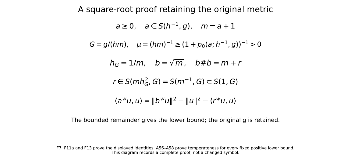
The diagram keeps the original and every factor in (F7), (F11a), (F13). Equations (A56)–(A58) prove the conformal comparison used here. This calculation uses the original conformal factor without a metric replacement.
10. Why the inverse square is the last uniform power
In one spatial dimension let and . The exact polynomial Weyl product is For a direct check, , whereas . Squaring the first expression gives the second plus .
Choose a nonzero real and, for , set Each function is smooth with compact support away from zero. Substituting gives For one fixed sufficiently large , (F42) is strictly negative. This is an independently chosen logarithmic test family; it uses no spectral assertion about the dilation generator.
Let be smooth, compactly supported on phase space, and equal to one near zero. Put . Then as : the convergence is pointwise and bounded by a fixed quartic polynomial, so dominated convergence applies against each Schwartz function. Pairing with the Wigner function of the fixed yields Fix , and define , with constant metric . Then , and Thus every relevant symbol seminorm is uniform, but the quadratic form in (F46), multiplied by , tends to minus infinity. A fixed positive rescaling of can make any prescribed finite list of these seminorms at most one; it does not change the divergence. No uniform theorem of the constant-metric form (F31) can replace by .
One can also put this obstruction into a single variable metric and a single symbol. This avoids interpreting a family of metrics as though it were one fixed operator. Still in one phase plane, take Choose the fixed integer sufficiently large. The summands then have disjoint supports, of radius at most a fixed multiple of , so the sum is locally finite and nonnegative. On each support is comparable to ; differentiating the summand proves . Slow variation of this metric follows from , and (F29), with , proves symplectic temperateness. Its uncertainty inequality holds.
Let be the unitary phase translation of the one fixed test function to . The contribution of the -th summand to its quadratic form is at most for large , by (F46). Every other contribution is negligible in absolute value. Here is a quantitative justification. The Wigner function of is Schwartz, and the kernel formula (F1) pairs it with the symbol, up to the fixed factor . For any integer , the absolute contribution of the -th summand with is at most The power in the volume factor is the area of its phase-space support. The chosen growth of the centers makes that support’s radius negligible relative to the distance between different centers. For , the sum of (F49) is at most ; for , it is at most . Taking makes both bounds tend to zero. The fixed norm of therefore accompanies a quadratic form tending to minus infinity. Thus the general theorem with , , fails even for one permissible metric and one nonnegative scalar symbol.
The example concerns scalar Weyl positivity and the uniform exponent. It neither gives an operator-valued Fefferman–Phong theorem nor supplies the separate matrix counterexamples needed to classify that setting.
11. Examples separating the assumptions
Subtracting a constant from a positive square. The operator is nonnegative on Schwartz functions, and its Weyl symbol is . Subtracting leaves the nonnegative symbol , but its operator has negative test forms by (F42)–(F44). Positivity of a function and positivity of its quantization are two different statements even for a polynomial.
A singular zero set without a positive Hessian. The function has both value and Hessian zero at the origin. The adaptive scale there is at its floor. The proof does not invoke an implicit critical graph with a nonzero Hessian at that point. It uses an ordinary bounded-symbol estimate on that scale, while nearby points with a larger value or Hessian can use the splitting argument. This is why the theorem includes arbitrarily degenerate zeros.
A classical symbol at a nonclassical derivative scale. Let , , and let be smooth on with every derivative bounded. In one dimension, belongs to if is smooth with compact support. To check the frequency derivatives, every derivative of the composed argument produces a factor bounded on by ; subsequent derivatives improve this bound. An derivative costs at most . The product rule gives the asserted class. Since , (F40) applies. This example illustrates the derivative accounting; the theorem is not restricted to such separated symbols or to compact support in .
12. Problems and complete solutions
Problem 1. For a constant metric on one phase plane, compute its dual and Planck parameter. Find a symplectic dilation making its two coefficients equal.
Solution. Formula (F2) gives , so . Under , the coefficients become and . Taking makes both equal to . The map preserves ; its unitary action on functions is the corresponding normalized dilation. Thus arbitrary eccentricity does not enter the constant-metric lower bound.
Problem 2. Why does a single square-root argument applied naively to at size fail to prove the second line of (F5)?
Solution. For a general nonnegative symbol of that size, the first-derivative positivity estimate is . The natural conformal metric that makes its own weight is then . Its Planck parameter is , which can exceed one near a zero of . The Weyl square remainder also has weight , which need not be bounded. The scalar splitting and dimensional reduction resolve precisely this failure; a formal square root alone does not.
Problem 3. Verify the cancellation in (F23) and state the remaining weight when has weight .
Solution. The Leibniz rule gives . Scalar multiplication commutes, so it cancels . The first surviving terms contain two symplectic contractions. Their weight is , both for the direct second correction and for the composition of two first corrections. That is why the localization error is bounded in .
Problem 4. Suppose satisfies (F25) and is defined by (F26). Explain both inequalities , and compute the rescaled -th derivative in (F27).
Solution. The maximum defining is at least one. Its other two entries are at most , by the order-zero and order-two bounds in (F25); since , the maximum is at most . Thus . The chain rule gives . For , its norm is at most . The lower derivative bounds instead use nonnegativity and the jet lemma; (F25) alone would give negative powers of there.
Problem 5. For the logarithmic family (F43), prove the negative-form condition and explain why one fixes before letting tend to zero.
Solution. Equations (F42) and (F44) give , negative when . Fix such an . Its Wigner function is now one fixed Schwartz test function, so the distributional convergence in (F45) gives (F46) directly. Letting the test function change with would require a separate uniform convergence estimate; none is needed for this counterexample.
Problem 6. A localized splitting has a profile independent of one phase direction but supported only on a transverse ball. Describe a global extension preserving the direction independence and nonnegativity, and explain why cutting off in all phase directions at that step is unsuitable.
Solution. Project the compact support of onto the orthogonal complement of the constant direction. This projection lies strictly inside the transverse domain on which is defined. Choose a nonnegative transverse cutoff equal to one near this projection and supported inside that domain. Multiply by it and extend by zero in the transverse variables; leave the constant direction unrestricted. The extension is smooth, nonnegative and independent of that direction, and satisfies . The later factor supplies the remaining localization in (F33). A cutoff varying in the missing direction would destroy the parameter decomposition used in dimension induction.
13. Exact source comparisons and visible corrections
The following is a separate editorial comparison, keeping the preceding scalar theorem and proof intact. It compares Wen Deng, Structure constants of the Weyl calculus, arXiv:1109.4793v1, with the original course formulas (F1)–(F5) and (F42). The source’s own wording and valid theorem remain identifiable. The two source-text corrections below are not errors in the course’s independent scalar proof. The original author files have not been edited.
The original source uses a measurable positive quadratic metric, the symplectic form , a continuous confined-symbol partition and imported Wiener and biconfinement theorems. The comparisons below apply on that common measurable-metric scope. They do not use the source to certify a larger nonmeasurable scope or to supply the missing proofs in its cited books.
13.1. Every Fourier and metric factor in the comparison
Keep the original course symbol , its original metric , original symplectic form and Lebesgue measure. Put and introduce only the comparison map For a Schwartz symbol and test function, substitution in the absolutely convergent source quantization gives For a tempered symbol the same identity is an equality of distributional kernels. Here is the exact extension, rather than an ordinary integral assertion: the partial Fourier transform is a continuous bijection of the Schwartz space and its distribution dual, and the coordinate change is invertible. They define both kernel maps continuously on tempered symbols. The distribution pullback under is . Applying these continuous maps to this identity gives precisely (SD2), including its . Equivalently one may test against the Schwartz Wigner function of two Schwartz functions; the same substitution has the same determinant. The complete Fourier, linear-substitution and distribution maps are already proved in the course prerequisites cited before (F2).
For all vectors , . Write , meaning . Its original symplectic dual is The second line uses the exact rule for , proved directly from the quotient defining the dual. Thus is equivalent to the original . The map has not replaced the original metric in the course calculation.
The original course quantity is . The source quantity is the reciprocal ratio, not the same quantity: The positive ratios attain finite positive extrema on a Euclidean unit sphere; reciprocating therefore changes their supremum into the reciprocal infimum. This also proves the identity at every base point without an exceptional zero or infinite value.
For the exact order- directional seminorm, with the original weight , the full comparison is A -unit vector maps to a vector of original -length ; each of the arguments contributes that factor. Conversely every such original vector is obtained by the inverse map. The weight has unchanged value at the corresponding point. For the source maximum through order , the exact expression is , bounded by . Do not substitute that upper bound for the exact maximum.
Slow variation retains its full radius: if has comparison constant for original squared distance at most , then the same comparison applies when . In the original distance . A one-base temperateness power consequently retains the factor as an upper bound when expressed with . Section2 below gives the exact comparison with the source’s harmonic-mean distance. Together (SD2)–(SD5) identify the lower-bound conclusions on their common scope with finite structural and symbol constants retained.
The polynomial correction is equally explicit. With the original , let . Original (F42) gives . The source operator for the unscaled coordinate symbol is , and Here and linearity supply the factor ; no square constant has been deleted or identified with a differently scaled symbol.
13.2. The exact two-way temperateness map
Let . Suppose the original (F3) holds in its actual orientation: For minimize under . In the original symmetric positive matrices the unique critical point and minimum are To prove the minimum, expand , complete the square with matrix , and retain the remaining matrix . It equals . Its inverse is ; this proves (SD8) without commuting the original matrices.
Put . The orientation of (SD7) gives . Duality gives . A second application gives Also . Since , multiplication gives the complete source-distance bound The source orientation with on the left follows by interchanging ; the mean is symmetric. Conversely choose in the minimum: , and choose to obtain the separate bound by . Therefore a harmonic-mean temperateness bound with constant and power implies (SD7) with and . This proves both maps, including the case .
13.3. The corrected quadratic-cutoff derivatives and their full receiver
In source Section2, original TeX line223 misses a factor2. Fix the original base , positive quadratic form , its associated inner product, original radius , and the actual smooth nonincreasing cutoff , with for arguments at most , for arguments at least1, and . Write , , and . The exact first derivative is Indeed . This is fixed by the original quadratic form; changing the meaning of its associated inner product would change the original data.
For every , the entire repeated-direction formula is Taylor-expand the original through order in the increment . The order- power contributes to only by choosing linear factors and quadratic factors. Multiplying its coefficient by , including the Taylor , gives exactly (SD11). The Taylor remainder is , so this coefficient calculation proves the derivative even where some factors vanish. At order zero the expression is just .
Every mixed direction is retained as well. If denotes the set of partitions of whose blocks have size1 or2, then All derivatives of of order at least3 vanish. Repeated differentiation of the product adds the new index either as a singleton differentiating , or to a singleton block differentiating . These choices generate each new partition exactly once; adjoining it to a double block gives zero. This proves (SD12) by induction and proves the full mixed formula without omitting multiplicities.
For define the actual finite coefficient sum On the support of a nonzero term, . Cauchy–Schwarz gives . Thus every original power in (SD11) gives The last comparison applies slow variation at base , on the very support just identified. In (SD12) each singleton contributes at most and each double block at most . The exact mixed bound is the sum over , with coefficient . Therefore the source’s estimates with unspecified finite constants keep their stated order and support after the equality is corrected; the omitted2 is restored in the constants explicitly.
The complete continuous-partition receiver keeps its original measure: Its lower bound is . To prove it, where the comparison integrand is nonzero, , so , , and monotonicity of applies. Substitution has the full Jacobian , proving that bound. The integral is positive since on the ball .
On the original support, and . Hence Here is the actual Euclidean unit-ball volume; it has not been absorbed into another object. Differentiation under the integral is justified even for the source’s measurable metric. Fix , take , and consider a nonzero cutoff derivative. Two slow comparisons give comparable with by , and . Thus the integration support lies in one finite ellipsoid, the determinant density is at most , and (SD12) gives a fixed integrable bound for every prescribed derivative on that neighborhood. For fixed the integrand is smooth in ; dominated convergence and the integral form of the difference quotient prove each derivative and its continuity. No differentiability of was used.
The positive lower bound permits the full reciprocal chain formula where contains all set partitions. Differentiating gives ; the same partition induction proves this formula. All its bounds are finite by (SD16) and the lower bound. The full product rule for therefore gives the original smooth partition bounds. Finally , with its original support and measure unchanged. This supplies the entire receiver of the corrected derivative, rather than only a first-order observation.
13.4. The literal Wiener-domain defect and a proved ambient repair
Source lines541–543 first restrict to Schwartz functions and then assert inclusion of all bounded smooth symbols with bounded derivatives. The original constant disproves that literal inclusion: it has every required bounded derivative, but , so it is not Schwartz. It does not contradict the intended localized Fourier condition.
Keep the original dimension , original compact smooth lattice cutoff , original locally finite partition , and original Fourier convention . For a tempered distribution introduce the separate ambient class Each compactly supported distribution has a smooth Fourier transform of polynomial growth: differentiate its action on the smooth exponential multiplied by a fixed compact test cutoff equal to one on its support. The distribution’s finite-order bound on that compact set proves the asserted polynomial estimate for every derivative. Thus the countable supremum in (SD18) is measurable and the definition is meaningful. This is explicitly an editorial ambient-domain repair, not a silent alteration of the source’s declaration.
For , translation gives To prove its integrability and the full finite-derivative inclusion, let have all coordinate derivatives through that order bounded. Write For , the transform has absolute value at most , uniformly in . For , choose with . The full product derivative and integration by parts give and hence . Every derivative term and its multiplicity has been retained. The actual polar measure gives In particular all symbols lie in the repaired ambient class, and taking proves the finiteness in (SD19). The same proof holds for bounded weak derivatives through order , using the already proved weak product rule and distributional integration by parts. It does not infer the imported fourth-derivative scalar lower-bound theorem from Fourier integrability alone.
For completeness the ambient repair has the actual functional properties needed to state its inclusion. Let , let , and put . There are at most nonzero partition terms at any point: if one index meets that point, every other index differs from by an element of . Fourier inversion in (SD18) makes each a continuous bounded function, with norm at most . Summing the locally finite partition identifies as a continuous bounded function and proves If the latter quantity is zero every vanishes, so the distribution vanishes. Triangle inequality and homogeneity follow from the countable supremum and the integral; the original quantity is a norm.
For a Cauchy sequence in this norm, (SD23) gives a uniform limit . Each converges uniformly on its fixed compact support, so its Fourier transform converges pointwise to that of . At fixed , the supremum of their pointwise limits is at most the lower limit of the suprema. Fatou’s lemma gives . It follows that belongs to the class and that in its original norm. Thus this repaired ambient space is complete.
For in it the product is their actual continuous-function product. In the localized identity , only indices with occur. Fourier transform of each product is convolution with no multiplier under . Each convolution is bounded by ; the complete finite sum therefore gives Tonelli justifies the convolution integral and retains its full factor . The original norm has not been rescaled to suppress that factor. These proofs establish bounded continuous representatives, completeness and continuous multiplication for the explicit ambient repair. The source’s separate imported Wiener-based sharp fourth-derivative theorem and its imported biconfinement bounds remain distinct literature dependencies.
13.5. Precise receiving and historical scope
The accompanying diagram is an exact two-dimensional sample of Section3. Its original matrix is , radius , displacement , and direction . The positive first pivot and determinant prove positivity. Direct multiplication gives , so this constant metric also satisfies uncertainty and slow variation with . The original line has and derivative . The displayed orange arrow is exactly , not a unit-vector replacement.
For this sample only, the diagram chooses , where for , zero otherwise, and . Every right derivative of at zero is the limit of an exponential times a polynomial in , hence vanishes, since each power times tends to zero. Thus is smooth and flat there. The denominator is everywhere positive, and . Consequently this particular cutoff is smooth, nonincreasing, equal to1 for and zero for . It is one admissible instance of the original cutoff hypotheses; (SD10)–(SD17) still hold for every original cutoff satisfying those hypotheses. The solid derivative curve uses the complete (SD10), while the dashed source expression is exactly half that value.
(SD1)–(SD9) prove the exact symbol, operator, metric, reciprocal-parameter and distance maps relating original (F1)–(F5) and (F42) to the cited source theorem. (SD10)–(SD17) restore the derivative equality and propagate it through every cutoff order and the full continuous-partition receiver. (SD18)–(SD24) disprove only the literal Schwartz-domain inclusion and supply the explicit repaired ambient space and the full finite-derivative inclusion, with all original Fourier and lattice factors.
No original course scalar theorem is replaced. Its original discrete cover, scalar splitting, dimensional induction, squared localization and logarithmic test remain the current independent proof. The exact version compared here is Deng1109.4793v1, submitted22September2011; its complete TeX and included bibliography were read. Its imported book theorems have not been reconstructed from their original-author TeX here. The two corrections are visible source notes, with their complete arguments above.
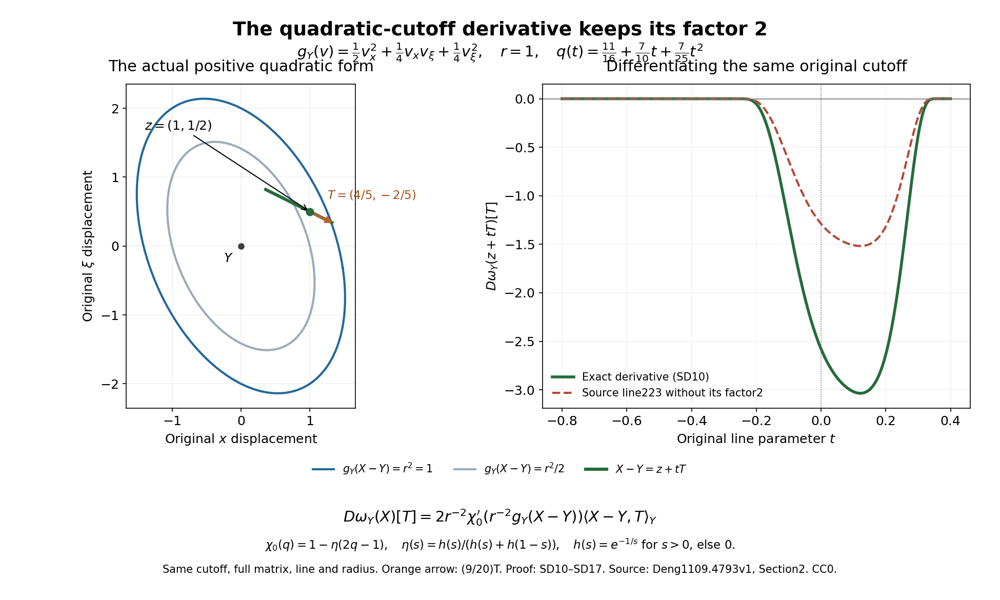
The left panel retains the complete matrix, both original ellipsoids, the displacement and direction. The right panel shows the exact derivative and the source expression with its missing factor2; the caption identifies the drawn arrow as (9/20)T. The exact sample and its smooth cutoff are proved in Section13.5.
References
Wen Deng’s Structure constants of the Weyl calculus, arXiv:1109.4793v1, Theorem 4.1, states the general-metric scalar bound on its declared measurable-metric scope, with dependence on the metric’s structural constants made explicit. Section13 proves the exact operator and metric comparison and records the two visible source corrections. Its proof uses a constant-metric result formulated through fourth derivatives in a Wiener algebra, followed by confined-symbol localization.
Nicolas Lerner’s author-hosted Metrics on the Phase Space, chapter 2, Theorems 2.5.5 and 2.5.10 and Remarks 2.5.13–14, discusses the general-metric bound and finer fourth-derivative conditions. Its reciprocal Planck parameter and -Fourier convention differ from (F1)–(F2). In particular constants in a polynomial Weyl-square identity must be converted before comparison.
Further questions
One direction for further work is an explicit, economical derivative count in (F37) for a specified class of metric structural constants. Another is to compare the sufficient pointwise condition with averaged conditions for a lower bound. Formula (F42) and the logarithmic tests show that quantization can produce a bounded negative quadratic form from a nonnegative scalar symbol. Sufficient averaged conditions require a separate theorem; they do not follow by deleting nonnegativity from the splitting lemma. A third direction is to identify exactly where scalar multiplication and the scalar critical graph cease to work for matrix symbols. The general Hilbert-valued sharp lower bound belongs to its separate course unit, and an inverse-square improvement in that setting cannot be inferred from this scalar proof.