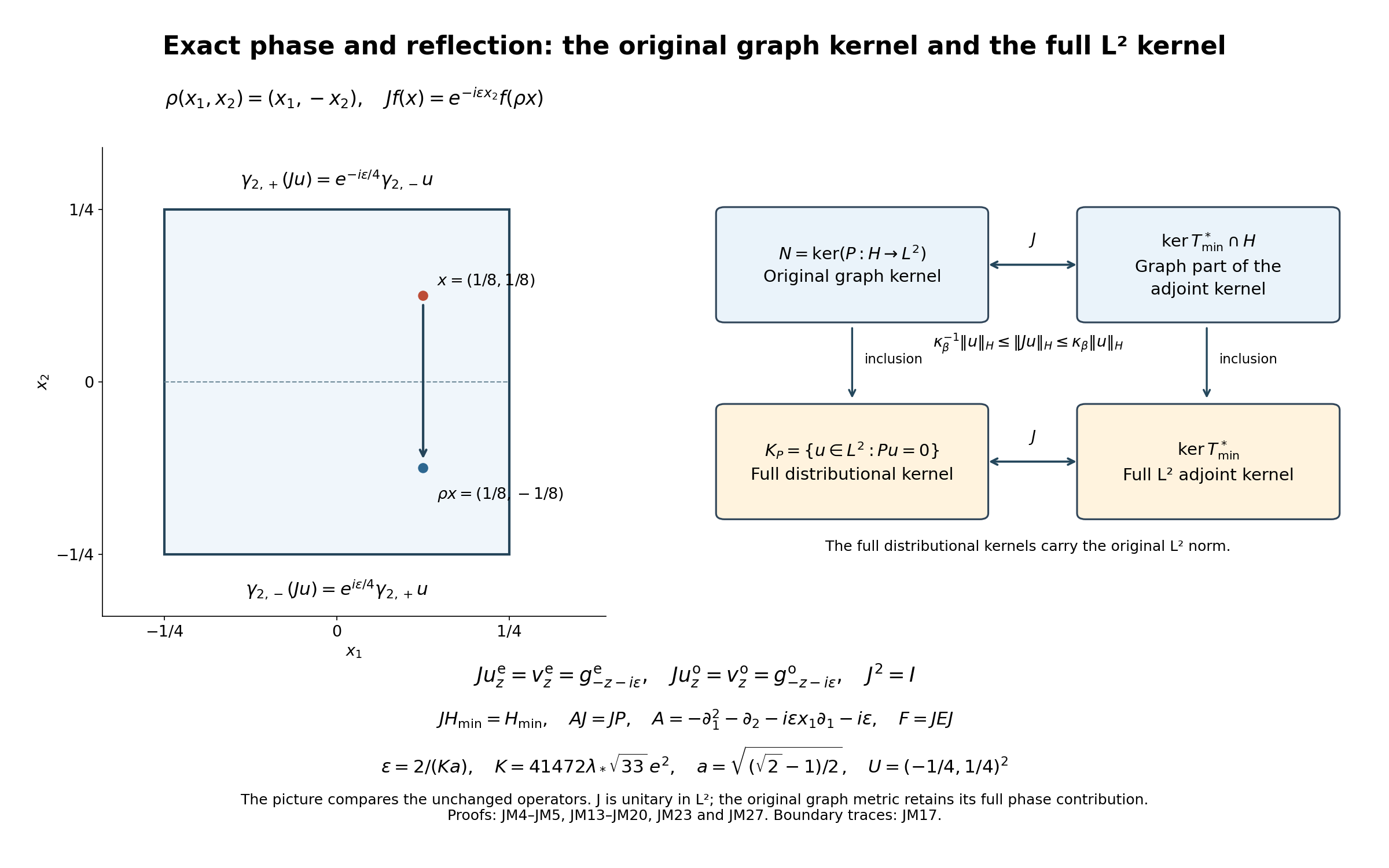
Exact reflection and phase transport for the original operator

This separate reflection and adjoint supplement proves an exact transport for the original operator. Its complete graph-domain foundations are in The two graph-domain quotients of the local inverse. The receiving original-source proofs are Local inverse, Section 14.6, (CS40)–(CS50) and Section 14.8.5, (CE25)–(CE34). The complete packaged proofs are the local inverse identities and the original-coefficient example. The pinned source citations require repository access. No new external theorem is used, and no novelty is claimed.

All Hilbert inner products below are linear in their first argument. Distribution pairings are complex bilinear. The resulting distinction between the Hilbert adjoint and distributional transpose is retained explicitly.

1. Fixed quantities and the involution on functions and distributions

Keep the original coordinates and all constants:

$$U=(-1/4,1/4)^2,\qquad D_j=-i\partial_{x_j},\qquad p(\xi_1,\xi_2)=\xi_1^2+i\xi_2,$$ $$C=\begin{pmatrix}14&-20&7\\-20&32&-12\\7&-12&5\end{pmatrix}, \quad\lambda_*=\text{the largest eigenvalue of }C,\quad K=41472\lambda_*\sqrt{33}\,e^2,\quad a=\sqrt{\frac{\sqrt2-1}{2}},\quad \varepsilon=\frac2{Ka}>0 . \tag{JM1}$$

Let $Y=L^2(U)$. For every polynomial $q$, keep its complete derivative strength $$\widetilde q(\xi)^2=\sum_{\alpha\in\mathbb N^2} |\partial_\xi^\alpha q(\xi)|^2, \quad V_p=\{q:\sup_{\xi\in\mathbb R^2}\widetilde q(\xi)/\widetilde p(\xi)<\infty\}, \quad \|q\|_p=\sup_{\xi\in\mathbb R^2}\frac{\widetilde q(\xi)}{\widetilde p(\xi)}.$$ For any actual declared basis $q_1,\ldots,q_4$ of the exact space $V_p$, define $$H=\{u\in L^2(U):q_j(D)u\in L^2(U),\ 1\leq j\leq4\}, \quad \|u\|_H^2=\|u\|_2^2+\sum_{j=1}^4\|q_j(D)u\|_2^2, \quad H_{\min}=\overline{C_c^\infty(U)}^{\|\cdot\|_H}. \tag{JM2}$$ The complete proofs of finite dimension, Hilbert completeness, $V_p=\operatorname{span}\{1,\xi_1,\xi_1^2,\xi_2\}$, and the four monomial norms are GM1–GM2 and GM31 of the retained note. No norm for a different basis is substituted for (JM2).

Retain the original full operator and its full Hilbert formal adjoint: $$P=D_1^2+iD_2+\varepsilon x_1D_1 =-\partial_1^2+\partial_2-i\varepsilon x_1\partial_1,$$ $$A=P^\dagger =D_1^2-iD_2+\varepsilon x_1D_1-i\varepsilon =-\partial_1^2-\partial_2-i\varepsilon x_1\partial_1-i\varepsilon. \tag{JM3}$$ The zeroth-order term is the contribution from $D_1(\varepsilon x_1 v)=\varepsilon x_1D_1v-i\varepsilon v$. It is retained in every calculation below. For this specific smooth coefficient, both expressions act on every distribution; this does not assert that an arbitrary continuous coefficient can multiply any distributional derivative.

Put $$\rho(x_1,x_2)=(x_1,-x_2),\qquad Jf(x_1,x_2)=e^{-i\varepsilon x_2}f(x_1,-x_2). \tag{JM4}$$ The real reflection has determinant $-1$, absolute Jacobian $1$, and preserves the actual open square. Since $\varepsilon$ is real, its displayed phase has modulus one. Thus change of variables, with Lebesgue measure and the absolute Jacobian retained, gives $$\langle Jf,Jh\rangle_2 =\int_U e^{-i\varepsilon x_2}f(x_1,-x_2) e^{i\varepsilon x_2}\overline{h(x_1,-x_2)}\,dx_1\,dx_2 =\langle f,h\rangle_2 .$$ Applying the exact phase twice gives $$J^2f(x) =e^{-i\varepsilon x_2}e^{-i\varepsilon(-x_2)}f(x)=f(x), \qquad \|Jf\|_2=\|f\|_2,\qquad J^*=J . \tag{JM5}$$ Consequently $J$ is a complex-linear unitary involution on $Y$.

Its distributional extension is specified by the actual bilinear transpose: $$\langle JT,\phi\rangle_{\mathcal D',\mathcal D} =\langle T,J^{\mathrm t}\phi\rangle_{\mathcal D',\mathcal D}, \qquad J^{\mathrm t}\phi(x_1,x_2) =e^{i\varepsilon x_2}\phi(x_1,-x_2). \tag{JM6}$$ The test transform maps $C_c^\infty(U)$ continuously to itself; reflection preserves compact support, and differentiation of its smooth phase leaves a finite sum of smooth bounded factors on each compact set. Formula (JM6) therefore defines a distribution for every $T$. For an $L^2$ function, the substitution $x_2\mapsto-x_2$ in its bilinear integral gives precisely this formula, so it agrees with (JM4). The test transform also squares to the identity, because its phases are $e^{i\varepsilon x_2}$ and $e^{-i\varepsilon x_2}$. Thus $J^2=I$ on distributions. In particular the plus sign in $J^{\mathrm t}$ is not replaced by the minus sign of the function formula or by the Hilbert adjoint convention.

For smooth functions, differentiation retains the complete phase contributions and gives $$D_1J=JD_1,\qquad D_2J=J(-D_2-\varepsilon),\qquad x_1J=Jx_1 . \tag{JM7}$$ Indeed differentiation of $e^{-i\varepsilon x_2}$ contributes $(-i)(-i\varepsilon)e^{-i\varepsilon x_2}=-\varepsilon e^{-i\varepsilon x_2}$; differentiation of the reflected argument contributes $i e^{-i\varepsilon x_2}(\partial_2f)(x_1,-x_2)$. Together these are exactly the second formula. The other coordinate and multiplication formulas follow because neither its phase nor its reflection changes $x_1$.

These formulas also hold on all distributions, without a regularity premise. In the bilinear convention $D_j^{\mathrm t}=-D_j$. On tests, direct differentiation of the plus-phase transform gives $D_1J^{\mathrm t}=J^{\mathrm t}D_1$ and $D_2J^{\mathrm t}=J^{\mathrm t}(-D_2+\varepsilon)$. For the second distributional identity, pair its left side against $\phi$ to obtain $\langle T,J^{\mathrm t}(-D_2\phi)\rangle$. The right side pairs as $\langle T,(D_2-\varepsilon)J^{\mathrm t}\phi\rangle$, which is the same expression by the displayed test identity. The first and multiplication identities follow by the same transpose calculation. Thus no differentiation or coefficient term is lost in their distributional extension.

2. The full weaker-polynomial pullback and every basis graph bound

Define the original affine frequency transform $$\tau(\xi_1,\xi_2)=(\xi_1,-\xi_2-\varepsilon),\qquad q^\#(\xi)=q(\xi_1,-\xi_2-\varepsilon).$$ It is an involution. Applying (JM7) successively to each monomial, then adding every coefficient, gives on all distributions $$q(D)J=Jq^\#(D),\qquad \partial_\xi^\alpha q^\#(\xi) =(-1)^{\alpha_2}(\partial_\xi^\alpha q)(\tau\xi), \qquad \widetilde{q^\#}(\xi)=\widetilde q(\tau\xi). \tag{JM8}$$ The chain rule has no additional higher-order term, because $\tau$ is affine with linear part $\operatorname{diag}(1,-1)$. Iterating the first-order chain rule proves the sign $(-1)^{\alpha_2}$ for every multi-index, including zero derivatives.

The full original $p$-strength at the reflected and translated frequency is $$\widetilde p(\tau\xi)^2 =\xi_1^4+(\xi_2+\varepsilon)^2+4\xi_1^2+1+4. \tag{JM9}$$ This contains the nonzero translated-frequency contribution and both separate constants $1$ and $4$. To compare it with the original array, the complete derivative array of $p^\#=\xi_1^2-i\xi_2-i\varepsilon$ is the array of $\overline p=\xi_1^2-i\xi_2$ with the additional zeroth entry $-i\varepsilon$ and no additional derivative entries. The two arrays have exactly the same first and second derivative entries and all the same zeros. The Euclidean triangle inequality therefore gives $$\widetilde p(\tau\xi)\leq\widetilde p(\xi)+\varepsilon \leq\left(1+\frac{\varepsilon}{\sqrt5}\right)\widetilde p(\xi), \qquad \widetilde p(\xi)\geq\sqrt{1+4}=\sqrt5 .$$ For $q\in V_p$, keep every factor in $$\widetilde{q^\#}(\xi) =\widetilde q(\tau\xi) \leq\|q\|_p\,\widetilde p(\tau\xi) \leq\left(1+\frac{\varepsilon}{\sqrt5}\right) \|q\|_p\,\widetilde p(\xi). \tag{JM10}$$ Thus $q^\#\in V_p$, with the exact proved bound $\|q^\#\|_p\leq(1+\varepsilon/\sqrt5)\|q\|_p$. Applying it again to $q^\#$ yields $\|q\|_p\leq(1+\varepsilon/\sqrt5)\|q^\#\|_p$, because $(q^\#)^\#=q$. This proves both directions of the comparison while retaining the original polynomial as the receiving object.

Let the column of original monomials be $r=(1,\xi_1,\xi_1^2,\xi_2)^{\mathrm T}$. For the actual basis in (JM2), write its exact coefficient matrix as $q=B_0r$, where $B_0\in\operatorname{GL}_4(\mathbb C)$. No coefficient of this basis matrix is discarded. The pullback has the full matrices $$r^\#=B_\#r,\qquad B_\#= \begin{pmatrix} 1&0&0&0\\ 0&1&0&0\\ 0&0&1&0\\ -\varepsilon&0&0&-1 \end{pmatrix},\qquad q^\#=\beta q,\qquad \beta=B_0B_\#B_0^{-1},\qquad \beta^2=I_4 . \tag{JM11}$$ The last row retains the translation term $-\varepsilon$. The other zero entries are retained in the printed matrix. The basis formula follows by inserting $r^\#$ into $q^\#=B_0r^\#$. The involution formula follows either by multiplying $B_\#^2=I_4$ or by applying the polynomial involution twice.

For $u\in H$, (JM8) and (JM11) give $q_j(D)Ju=J\sum_k\beta_{jk}q_k(D)u$. Every right side is an $L^2$ function, which proves $Ju\in H$. Exact $L^2$ unitarity then gives the original-norm identity $$\|Ju\|_H^2 =\|u\|_2^2 +\sum_{j=1}^4 \left\|\sum_{k=1}^4\beta_{jk}q_k(D)u\right\|_2^2. \tag{JM12}$$ Put $\sigma_\beta=\|\beta\|_{\mathbb C^4\to\mathbb C^4}$, with the ordinary Euclidean coefficient-vector norm, and $\kappa_\beta=\max\{1,\sigma_\beta\}$. The definition of this finite matrix norm and integration imply $$\kappa_\beta^{-1}\|u\|_H \leq\|Ju\|_H\leq\kappa_\beta\|u\|_H, \qquad J:H\longrightarrow H\text{ is a bounded involution.} \tag{JM13}$$ The upper estimate uses (JM12) and its unchanged separate $L^2$ term. Apply it to $Ju$ and use $J^2u=u$ for the lower estimate. If a directly summed finite bound is desired, $\sigma_\beta\leq(\sum_{j,k}|\beta_{jk}|^2)^{1/2}$ follows by rowwise Cauchy–Schwarz; every actual basis coefficient remains in that sum.

For the declared monomial basis of GM32, $B_0=I_4$, so $\beta=B_\#$. The actual graph norm has its two separate $u$ terms: $$\|Ju\|_H^2 =\|u\|_2^2+\|u\|_2^2+ \|D_1u\|_2^2+\|D_1^2u\|_2^2+\|D_2u+\varepsilon u\|_2^2$$ $$=\|u\|_H^2+\varepsilon^2\|u\|_2^2 +2\varepsilon\operatorname{Re}\langle D_2u,u\rangle_2. \tag{JM14}$$ The matrix coefficient norm has squared value $\sigma_\beta^2=1+\varepsilon^2/2+ (\varepsilon/2)\sqrt{\varepsilon^2+4}$: the nontrivial block of $\beta^*\beta$ is $\begin{pmatrix}1+\varepsilon^2&\varepsilon\\\varepsilon&1\end{pmatrix}$; its characteristic polynomial gives these two eigenvalues with signs plus and minus, and the other two eigenvalues are one.

Keeping the separate duplicate $u$ terms gives the stronger proved bound $$k_H^2=1+\frac{\varepsilon^2}{4} +\frac{\varepsilon}{4}\sqrt{\varepsilon^2+8}, \qquad k_H^{-1}\|u\|_H\leq\|Ju\|_H\leq k_H\|u\|_H. \tag{JM15}$$ Here is a direct verification in the original metric. For a pair of complex numbers $b,d$, the relevant input expression is $|b|^2+|b|^2+|d|^2$, and its output is $|b|^2+|b|^2+|d+\varepsilon b|^2$. Their Hermitian matrices are respectively $\operatorname{diag}(2,1)$ and $\begin{pmatrix}2+\varepsilon^2&\varepsilon\\\varepsilon&1\end{pmatrix}$. The determinant of the difference with $t\operatorname{diag}(2,1)$ is $2(1-t)^2-\varepsilon^2t$. Its larger root is exactly $t=k_H^2$. At that root the matrix $$k_H^2\operatorname{diag}(2,1)- \begin{pmatrix}2+\varepsilon^2&\varepsilon\\\varepsilon&1\end{pmatrix}$$ has determinant zero and positive diagonal entries: the lower entry is $k_H^2-1>0$, and the upper is $(\varepsilon/2)(\sqrt{\varepsilon^2+8}-\varepsilon)>0$. Its quadratic form is nonnegative, because if the two positive diagonal entries are $\alpha,\delta$, their product is $\varepsilon^2$, and its form is $|\sqrt\alpha b-\sqrt\delta d|^2$. Thus the output pair is bounded by $k_H^2$ times the input pair. Integrate this bound and retain both other graph derivatives, whose norms are unchanged by $J$. Since $k_H^2\geq1$, they obey the same upper bound. Apply it to $Ju$ for the inverse estimate. This proves (JM15) as a bound in the original graph metric. It does not assert equality with the actual graph-operator norm, nor replace the original metric by the two-dimensional coefficient matrix.

3. The actual minimal domain and every trace phase

The map $J$ sends $C_c^\infty(U)$ onto itself: reflection preserves the square and compact support, and multiplication by its smooth phase preserves smoothness. By (JM13) both $J$ and its inverse are bounded on the actual $H$. If $u_j\to u$ in $H$ with compactly supported smooth $u_j$, then $Ju_j\to Ju$ in the same norm. Applying the involution for the reverse inclusion proves $$JH_{\min}=H_{\min}. \tag{JM16}$$

For the monomial basis, the six trace maps in GM55–GM56 have the exact transport $$\gamma_{1,\pm}(Ju)(x_2) =e^{-i\varepsilon x_2}(\gamma_{1,\pm}u)(-x_2), \qquad \gamma'_{1,\pm}(Ju)(x_2) =e^{-i\varepsilon x_2}(\gamma'_{1,\pm}u)(-x_2),$$ $$\gamma_{2,+}(Ju)=e^{-i\varepsilon/4}\gamma_{2,-}u,\qquad \gamma_{2,-}(Ju)=e^{i\varepsilon/4}\gamma_{2,+}u . \tag{JM17}$$ These are equalities in their actual $L^2(-1/4,1/4)$ trace spaces. To prove the vertical formulas, regard $u(x_1,\cdot)$ and $\partial_1u(x_1,\cdot)$ as the continuous Hilbert-valued representatives supplied by GM53. The phase-reflection transform on that $L^2$ space is a fixed unitary map independent of $x_1$. It therefore commutes with taking the endpoint limits of those two representatives. The derivative identity (JM7) gives the indicated first derivative as well. For the horizontal formulas, use the continuous representative $u(\cdot,x_2)$ in the other $L^2$ space; reflection changes the endpoint and the phase evaluates at the original endpoint $+1/4$ or $-1/4$, giving exactly the displayed factors. Thus every side and phase is accounted for. All six zero conditions are transported to themselves, with the horizontal sides exchanged, in agreement with (JM16). No trace of a missing mixed derivative is assumed.

4. The exact kernel bridges and the distinction between two adjoint domains

Using (JM7), with the zeroth-order term in (JM3) still present, gives on every distribution $$AJ =J\bigl[D_1^2+iD_2+i\varepsilon+ \varepsilon x_1D_1-i\varepsilon\bigr] =JP,\qquad PJ=JA. \tag{JM18}$$ The first equality shows the two separate $i\varepsilon$ and $-i\varepsilon$ contributions before their cancellation. The second intertwining follows by multiplying $AJ=JP$ on both sides by the involution. This is a proved comparison of the original two operators; neither is used as a replacement definition of the other.

Define the full distributional $L^2$ kernel and the actual graph kernel separately: $$K_P=\{u\in L^2(U):Pu=0\text{ in }\mathcal D'(U)\}, \quad N=\ker(P:H\to Y)=K_P\cap H,$$ $$N^\dagger=\ker T_{\min}^* =\{v\in L^2(U):Av=0\text{ in }\mathcal D'(U)\}, \qquad T_{\min}=P|_{H_{\min}}\text{ as an operator in }Y. \tag{JM19}$$ The adjoint-domain equality is proved in GM26. The first kernel is closed in $L^2$: if $u_j\to u$ there, every test pairing of $Pu_j$ converges to that of $Pu$, because distributional derivatives and multiplication by the specific smooth coefficient are continuous on distributions. Thus a sequence of zero pairings has a zero limit. The same argument applies to $N^\dagger$.

The distributional identity (JM18) proves $J K_P\subset N^\dagger$, and its reverse identity proves $J N^\dagger\subset K_P$. Using $J^2=I$ proves both surjectivity and inverse formulas. The map $$J:K_P\longrightarrow\ker T_{\min}^* \text{ is a complex-linear unitary bijection in the original }L^2\text{ norms}.$$ Preservation of $H$ then gives the strongest corresponding graph-domain bridge $$J:N\longrightarrow N^\dagger\cap H=\ker(A:H\to Y) \text{ is a bounded bijection with inverse }J,$$ $$\kappa_\beta^{-1}\|u\|_H\leq\|Ju\|_H\leq\kappa_\beta\|u\|_H \quad(u\in N), \qquad \|Ju\|_2=\|u\|_2. \tag{JM20}$$ For the monomial basis use the stronger $k_H$ bound (JM15). The spaces $N$ and $N^\dagger\cap H$ are closed in their $H$ norms because they are kernels of bounded maps $P,A:H\to Y$. For $A$, this boundedness follows directly from its polynomial terms and bounded smooth coefficients, or from $A=JPJ$, (JM13), and $\|P\|\leq C_P$. The broader $K_P$ is not silently identified with $N$. Likewise the full $N^\dagger$ is not silently identified with its intersection with $H$.

Let $A_{\min}$ mean the minimal graph closure in $L^2$ of the formal expression $A$ initially on $C_c^\infty(U)$. This is a different domain question from the Hilbert adjoint $T_{\min}^*$. Indeed unitary transport on $L^2$, the core transport $JC_c^\infty=C_c^\infty$, and (JM18) give $$A_{\min}=JT_{\min}J,\qquad \operatorname{Dom}(A_{\min})=JH_{\min}=H_{\min},$$ $$\operatorname{Dom}(T_{\min}^*) =\{v\in L^2(U):Av\in L^2(U)\text{ as a distribution}\}, \qquad T_{\min}^*v=Av. \tag{JM21}$$ For the closure assertion, the graph map $(u,Pu)\mapsto(Ju,JPu)$ is an isometry on $Y\oplus Y$; it maps the core graph of $P$ onto the core graph of $A$ by (JM18). It consequently maps their graph closures onto one another. GM-A1 identifies the first closure domain as $H_{\min}$, and (JM16) gives the displayed transported domain. This proves the first formula, including closedness and dense definition. The second formula retains the fully proved GM26 domain, rather than giving it the minimal trace conditions.

The actual inclusion $A_{\min}\subset T_{\min}^*$ follows from (JM21) since $u\in H_{\min}$ has all polynomial derivatives and hence $Au\in L^2$. It is proper. For example $u_0=1$ is a nonzero member of $N$ by GM45, so $Ju_0=e^{-i\varepsilon x_2}$ is a nonzero element of $N^\dagger\cap H$ by (JM18). It is in $\operatorname{Dom}(T_{\min}^*)$. It cannot be in $H_{\min}$, since (JM16) would put $u_0$ in $H_{\min}$, contradicting the injectivity estimate GM8 or its positive distance in GM46. Thus it is outside the domain of $A_{\min}$. This proves the specific strict inclusion, while making no unproved strict inclusion between $K_P$ and $N$.

5. The transported completed inverse, closed minimal range, and quotient maps

Retain $E:Y\to H$, $PE=I_Y$, and $EP=I$ on $H_{\min}$ from GM6–GM8 and the original (CS43)–(CS50). Let $$R=P(H_{\min}),\qquad R_A=A(H_{\min}).$$ The exact range transport and minimal graph-operator comparison are $$R_A=JR,\qquad A_{\min}(Ju)=J(T_{\min}u)\quad(u\in H_{\min}). \tag{JM22}$$ Indeed $J$ maps $H_{\min}$ onto itself and $AJ=JP$. This proves each range inclusion and their equality. Since $R$ is closed in $Y$ by GM-A and $J$ is unitary, $JR$ is closed.

Define the transported map using its full phases, rather than a new coefficient convention: $$F=JEJ:Y\longrightarrow H,\qquad AF=I_Y,\qquad FAu=u\quad(u\in H_{\min}),\qquad F(JR)=H_{\min}. \tag{JM23}$$ For boundedness, (JM13), exact $L^2$ unitarity on the input side, and $\|E\|\leq C_E$ give $\|Ff\|_H\leq\kappa_\beta C_E\|f\|_2$. The right-inverse formula is $AF=AJEJ=JPEJ=JJ=I$. For $u\in H_{\min}$, use $JAu=PJu$ and $Ju\in H_{\min}$ to give $FAu=JEPJu=JJu=u$. Finally $F(JR)=JE(R)=JH_{\min}=H_{\min}$, using the exactly proved GM8 image formula. Hence $$A_{\min}:H_{\min}\longrightarrow JR \text{ is a bounded bijection with inverse }F|_{JR}, \quad \|u\|_H\leq\kappa_\beta C_E\|Au\|_2\quad(u\in H_{\min}). \tag{JM24}$$ Its graph-domain operator norm is at most $\kappa_\beta C_P$ from $A=JPJ$. In the monomial basis, every coefficient gives the explicit independent bound $$\|A\|_{H\to Y} \leq C_A=\left(|-i\varepsilon|^2+ \varepsilon^2/16+|1|^2+|-i|^2\right)^{1/2}.$$ Its first coefficient is the retained zeroth-order term. The corresponding original constants are $$C_P=\left(|0|^2+\varepsilon^2/16+|1|^2+|i|^2\right)^{1/2}, \qquad C_E=2K\left(\frac15+\frac15+a^2+1+1\right)^{1/2}.$$ For that basis $\|F\|\leq k_H C_E$ and the coercive bound in (JM24) also improves to $k_H C_E$, using (JM15). Both copies of $1/5$ and both copies of $1$ remain present. The map $F$ is a right inverse of $A:H\to Y$ on every input; its inverse on the minimal realization is $F|_{JR}$. There is no claim that $Ff\in H_{\min}$ for $f\notin JR$.

The kernel projections are transported exactly: $$Q=I-EP,\qquad Q_A=I-FA=JQJ,\qquad \operatorname{Ran}Q_A=JN=N^\dagger\cap H,\qquad \ker Q_A=F(Y),\qquad Q_AH_{\min}=0. \tag{JM25}$$ The equality follows from $F=JEJ$ and $A=JPJ$. Its range, kernel and zero restriction follow by applying the original projection identities GM9–GM11 through the bijections $J:H\to H$ and $J:H_{\min}\to H_{\min}$. This also proves its idempotence. An explicit bound is $\|Q_A\|\leq\kappa_\beta^2(1+C_EC_P)$; the direct formula gives the additional bound $1+\kappa_\beta C_E\,\|A\|$. For the monomial basis use $k_H$ in place of $\kappa_\beta$ and the proved $C_A$ in the second bound. No orthogonality of the graph-domain summands is asserted.

There are exact quotient transports $$\mathcal J_H:H/H_{\min}\to H/H_{\min},\quad [u]\mapsto[Ju], \qquad \mathcal J_Y:Y/R\to Y/JR,\quad[f]\mapsto[Jf]. \tag{JM26}$$ The first is well defined by (JM16), involutive, and obeys both $\kappa_\beta$ bounds in the original quotient norm: take the infimum over $h\in H_{\min}$ in $\|J(u-h)\|_H$, then use the inverse. The second is well defined because $J(R)=JR$. Its inverse is the same formula in the opposite quotient spaces, and it is isometric: $$\inf_{m\in R}\|Jf-Jm\|_2=\inf_{m\in R}\|f-m\|_2.$$ The two actual quotient decompositions therefore commute with $J$: $$[Ju]\longmapsto(Q_AJu,[AJu]) =(JQu,[JPu]).$$ This is the transport of the original map $[u]\mapsto(Qu,[Pu])$ by $J|_N$ and $\mathcal J_Y$. The adjoint-side inverse is $(v,[f])\mapsto[v+Ff]$, which is well defined because $F(JR)=H_{\min}$. It is inverse by $AF=I$, $Q_AF=0$, and $u=Q_Au+FAu$; these are precisely the identities just proved. Moreover $(JR)^\perp=J(R^\perp)=J N^\dagger=K_P$. For its proof, $y\perp JR$ if and only if $Jy\perp R$ by unitarity, and then use the kernel bijection (JM19)–(JM20). Thus the adjoint-side obstruction quotient retains the full $L^2$ kernel of $P$; it is not reduced to $N$.

6. The exact entire mode phases and graph energies

Retain the complete even and odd functions from GM34 and GM47: $$\varphi_z(x_1)= \sum_{k=0}^\infty \frac{\prod_{h=0}^{k-1}(z-2i\varepsilon h)}{(2k)!}x_1^{2k}, \qquad \psi_z(x_1)= \sum_{k=0}^\infty \frac{\prod_{h=0}^{k-1}(z-i\varepsilon(2h+1))}{(2k+1)!}x_1^{2k+1}.$$ The empty products are one. Their complete compact convergence, every differentiated series, and actual graph-domain membership were proved in GM34–GM40 and GM47–GM48. With $$u_z^{\rm e}=e^{zx_2}\varphi_z(x_1),\qquad u_z^{\rm o}=e^{zx_2}\psi_z(x_1),$$ $$g_\lambda^{\rm e}=e^{\lambda x_2}\varphi_{-\lambda-i\varepsilon}(x_1),\qquad g_\lambda^{\rm o}=e^{\lambda x_2}\psi_{-\lambda-i\varepsilon}(x_1),$$ retain also the actual GM42 parametrization $$v_z^{\rm e}=e^{-(z+i\varepsilon)x_2}\varphi_z(x_1),\qquad v_z^{\rm o}=e^{-(z+i\varepsilon)x_2}\psi_z(x_1).$$ The exact full-parameter transport is $$Ju_z^{\rm e}=v_z^{\rm e}=g_{-z-i\varepsilon}^{\rm e},\qquad Ju_z^{\rm o}=v_z^{\rm o}=g_{-z-i\varepsilon}^{\rm o},\qquad Jg_\lambda^{\rm e}=u_{-\lambda-i\varepsilon}^{\rm e},\qquad Jg_\lambda^{\rm o}=u_{-\lambda-i\varepsilon}^{\rm o}. \tag{JM27}$$ For example the even left side is $$e^{-i\varepsilon x_2}e^{z(-x_2)} \sum_{k=0}^\infty \frac{\prod_{h=0}^{k-1}(z-2i\varepsilon h)}{(2k)!}x_1^{2k}.$$ Its full exponential is $e^{(-z-i\varepsilon)x_2}$. At $\lambda=-z-i\varepsilon$, the complete even $g$-coefficient is $-\lambda-i\varepsilon(2h+1)=z-2i\varepsilon h$. For the odd family its coefficient is $-\lambda-i\varepsilon-i\varepsilon(2h+1) =z-i\varepsilon(2h+1)$. Thus every product factor and factorial agrees with the respective original $u$ series; no phase is discarded. The reverse formulas follow by the same parameter calculation or $J^2=I$.

Exact $L^2$ unitarity gives equality of the two mode $L^2$ norms. The graph norms obey the more informative original-metric formula $$\|g_{-z-i\varepsilon}^{\rm e}\|_H^2 =\|u_z^{\rm e}\|_H^2+ (\varepsilon^2+2\varepsilon\operatorname{Im}z)\|u_z^{\rm e}\|_2^2,$$ $$\|g_{-z-i\varepsilon}^{\rm o}\|_H^2 =\|u_z^{\rm o}\|_H^2+ (\varepsilon^2+2\varepsilon\operatorname{Im}z)\|u_z^{\rm o}\|_2^2 \tag{JM28}$$ for the monomial metric GM32. Indeed $D_2u_z=-iz\,u_z$ in both families, so the cross term in (JM14) has real part $\operatorname{Re}(-iz)\|u_z\|_2^2=(\operatorname{Im}z)\|u_z\|_2^2$. Every other derivative term and both separate $u$ terms are unchanged. This proves the formulas, including when that correction is negative. Their full right sides remain nonnegative because they equal the actual squared graph norms with last derivative factor $|z+i\varepsilon|^2$. No graph unitarity is inferred from the $L^2$ unitarity.

Finally this comparison also transports the complete bounded solver choices proved in GM58–GM64. If $G:Y\to H$ satisfies $PG=I_Y$ and $GP=I$ on $H_{\min}$, then $$G_A=JGJ,\qquad AG_A=I_Y,\qquad G_AA=I\text{ on }H_{\min}, \qquad \|G_A\|\leq\kappa_\beta\|G\|. \tag{JM29}$$ The two identities follow by inserting $AJ=JP$, $JA=PJ$, and $JH_{\min}=H_{\min}$; the norm bound uses $J$’s $H$ bound on the output and its exact unitary input norm. The same conjugation is the inverse correspondence and gives the inverse bound. At $G=E$ it gives the already proved $F$.

If the original choice is $G=E+L\pi_R$, write $$G_A=F+L_A\pi_{JR},\qquad L_A=J|_N\,L\,\mathcal J_Y^{-1}: Y/JR\longrightarrow N^\dagger\cap H.$$ To verify this exact parameter formula, note that $\pi_RJ=\mathcal J_Y^{-1}\pi_{JR}$, since both send $f$ to $[Jf]$ in $Y/R$. Substitution gives $JGJ=JEJ+JL\pi_RJ$, exactly the displayed formula. Boundedness and its inverse use the isometry of $\mathcal J_Y$ and the two graph bounds of $J|_N$. Thus the comparison retains the original full solver parameters and transports them to the actual graph-domain adjoint kernels; it does not replace either original operator or confuse a minimal realization with its Hilbert adjoint.

The diagram accompanying this supplement labels both kernel bridges, the exact phase and reflection, and the original square’s trace transport. Its caption points to (JM4)–(JM5), (JM13)–(JM17), and (JM19)–(JM20). The graph-domain note supplies the complete earlier proofs. The bounded original-author TeX comparison records the earlier reading coverage; this supplement makes no additional human-source reading or exhaustive literature claim.