The two graph-domain quotients of the local inverse
This editorial note derives the graph-domain consequences of the completed local inverse. Its receiving proofs are Section 14.6, (CS40)–(CS50) and the unchanged example in Section 14.8.5, (CE25)–(CE34). The original lesson construction and the unchanged example remain explicit throughout. These source links require access to the course repository. The complete packaged proofs are the local inverse identities and the original-coefficient example.
All spaces below are complex. The inner product is linear in its first argument. Distribution pairings retain the complex-bilinear convention of U006. The Hilbert adjoint introduced below consequently involves conjugation; it is a different operation from the distributional transpose in U006 (CS4).
1. The unchanged polynomial graph space and completed maps
Retain the original nonzero polynomial , its degree , the original coordinates, and . For every polynomial , keep the full strength array
Every zeroth and higher derivative, including its zero value, remains part of this definition. To recall why its denominator is positive, choose a nonzero degree- coefficient . Then , so . For , this bound is . It follows that , with . The pointwise triangle inequality for the complete derivative arrays makes a vector space and a norm.
This vector space is finite dimensional. Indeed for some finite , since its derivative array is finite and each entry is a polynomial of degree at most . If had degree , its degree- part would be nonzero at some real vector . A polynomial zero on every real vector has every coefficient zero: apply the one-variable root bound in the first variable for each fixed choice of the other variables and repeat by induction. Consequently would contradict . Thus lies in the finite-dimensional space of polynomials of degree at most . These are also the arguments in U006 (CS5)–(CS6).
Choose the actual basis used for the graph norm. Retain the original polynomials , coefficients with , and the bounded open neighborhood of (CS42). In particular the coefficients are bounded on , because is compact. Put , and use exactly the full common maximal graph space
The derivatives in this definition are distributional. Its inner product is the corresponding sum of the original inner products. Completeness follows directly: if is Cauchy in this norm, let and be the limits of and . Testing against a compactly supported smooth function shows , because differentiation is continuous in the distributional topology and convergence implies distributional convergence by Cauchy–Schwarz. Thus and in . A basis expansion proves that the set contains the distributional derivative for every . No graph norm is changed when this fact is used.
Write the exact basis expansions
The graph-domain realization of the original operator is
Every coefficient multiplies an already defined function. Define the finite bound
Pointwise Cauchy–Schwarz followed by integration proves . This is an explicit bound, with every original coefficient present; sharpness of the operator norm is not claimed.
Keep the completed maps , and from (CS38)–(CS50), rather than constructing a new inverse. Keep
Equations (CS41), (CS45), and (CS47) give the bounded map with . Equation (CS48) proves ; equation (CS50) proves for . These are completed input results, with their full proofs retained in the input lesson. This note derives their domain consequences without adding a solvability premise or suppressing any part of their construction.
2. The minimal domain, its closed image, and the exact kernel projection
Define the actual minimal common graph domain by
Theorem GM-A. The identity holds on . The restriction is a bounded bijection with inverse , and
The image is closed in . The exact operator
is a bounded projection onto , with kernel , and
It vanishes on . The completed solution space is the exact topological direct sum
For every , all solutions in this original graph domain, and only those solutions, are
Proof. For , choose with in . Boundedness of gives in . Boundedness of then gives in . On the compactly supported functions the input identity is initially an equality in , and hence an equality in , since the equal classes have the same distributional derivatives. Taking the limit proves in . The estimate in (GM8) follows. It proves injectivity of ; surjectivity onto is its definition. If with , then . Conversely for every . Thus , and .
To prove closedness, let converge in to . Write . The bound for gives in . Since is closed, ; since , it follows that . This proves the claimed closedness without a Fredholm or ellipticity assumption.
The identity gives . Expanding proves . It also gives and . If , then , so the range of is exactly . If , then ; if , then . Thus the kernel is exactly . Both summands are closed: is the kernel of a bounded map, and is the kernel of . The intersection is zero, because implies . Formula (GM11) is the definition of . Its projections are and , so the direct sum is topological. The norm bound in (GM10) is the triangle inequality and the two operator bounds. Finally for ; any solution satisfies . This proves (GM12). ∎
Corollary GM-A1: the single-operator minimal closure. Consider on with its original expression (GM4). Its closure as an unbounded operator in has domain exactly , and it is injective with closed range . On this domain the original full graph norm and the single-operator graph norm obey
Proof. The second estimate holds on all of by (GM2) and (GM5); the first follows from (GM8). If converges in the single-operator graph norm, the difference version of (GM8) makes it Cauchy in the full original norm. Its limit is in and agrees with its limit, and boundedness of identifies the limiting image. Conversely the defining -approximation for gives approximation in the single-operator graph norm by the second estimate. This proves equality of the two closures while retaining both norms and their exact comparison.
For closedness as an unbounded operator, suppose , in , and in . Again (GM8) makes Cauchy in . Its limit belongs to , agrees with , and has image . The domain is dense in , because it contains , which is dense: truncate an function to compact subsets a positive distance from the boundary, then mollify with radii smaller than that distance. The truncations converge by dominated convergence, and the mollifications by translation continuity in . These operations are also proved in the prerequisite cited in U006 before (CS38). Injectivity and closed range were proved in GM-A. ∎
The word “maximal” in (GM2) refers to all original constant-polynomial derivatives in . We have not replaced that domain by a domain that asks only for . For continuous coefficients, multiplying an arbitrary distributional derivative by a coefficient is not automatically defined. The exact closure statement just proved applies to the minimal operator and supplies the bridge between its two graph norms without altering the maximal common domain.
3. The complete quotient maps, constants, and three projections
Equip and with their actual quotient norms:
On , use the Hilbert direct-sum norm
Theorem GM-B. The following explicit maps are inverse bounded linear isomorphisms:
Put . Their original-norm bounds are
The exact quotient norm, before using either estimate, is
There is also the split exact sequence with all original connecting maps
Proof. If is replaced by for , then and , so (GM16) is well defined. If is replaced by for , then , so (GM17) is well defined. Using , , , and , we obtain . Using (GM11), we obtain .
For every , Square, add, and take the infimum to obtain the first bound. For every , Taking the infimum and then applying two-variable Cauchy–Schwarz proves the second bound. Since , the infimum in the definition of the quotient norm is exactly (GM19), not a newly imposed norm. The injection in (GM20) is injective because . The second map is surjective because . If , then , so and is in the displayed injection. The splitting follows from and is bounded by . Thus every assertion of exactness and splitting is established. ∎
For completeness, a closed subspace of a Hilbert space has an orthogonal projection with norm at most one. Here is the argument used below. For , let , and choose approaching that infimum. The parallelogram identity gives Thus . The real one-variable variation of , first for , then for , proves . This orthogonal decomposition is unique, depends linearly on , and its two squared component norms add to ; consequently each projection has norm at most one. Write these projections as and .
There are three actual bounded projections on :
Their ranges are respectively , their pairwise products in both orders are zero, and their sum is . Indeed , the two orthogonal -projections square to themselves and have zero products, and . The range of is , and it is the identity there because on that domain. The same calculation proves the other range and identity. Thus
These sums use the original norm. Orthogonality between their -summands is not asserted. The precise quotient-coordinate map is also , because is an isometry from onto .
4. The second factor is the exact adjoint obstruction space
Define the original Hilbert formal adjoint distribution on by
The bars on polynomials conjugate their coefficients, not their variables. Each product inside a derivative is an function; distributional differentiation of that product is defined even when is only continuous. No derivative of a continuous coefficient is postulated as a function.
Theorem GM-C. One has . In particular the quotient factor is isometrically isomorphic to the exact distributional adjoint kernel, and the original full graph-domain quotient has the bounded isomorphism
with the bounds in (GM18), using the norm on and the norm on .
Proof. For , integration by parts or the definition of distributional derivatives gives
For the signs, , its distributional transpose is , and . The same identity term by term in the complete polynomials gives on and on . There is no boundary contribution because is compactly supported.
If , its pairing with vanishes for every such , so (GM25) proves . Conversely, if , the pairing vanishes on . For any , choose the original graph approximation . Then in , so Cauchy–Schwarz extends the zero pairing to . Hence . This proves equality. Since is closed, the orthogonal quotient identification proved after GM-B applies. Substitution in (GM16)–(GM17) gives (GM24) and its inverse, and all bounds are unchanged. ∎
The unbounded adjoint of the closed densely defined minimal operator of GM-A1 has the complete domain
To prove this, the defining adjoint equality on restricts to (GM25), and so identifies its representing function with . Conversely an representing function for gives the adjoint equality first on the compactly supported functions by (GM25), then on by graph approximation; both and in . This proves both inclusions of the domain and the displayed operator formula. Therefore the space in (GM24) is exactly , with no additional regularity condition.
There is an exact existence criterion for the minimal-domain solution: for , a solution of exists if and only if for every . In that event its unique value is . Indeed a minimal-domain image lies in and is orthogonal to . Conversely the orthogonal decomposition , proved above, shows that orthogonality to forces the second component to vanish, so . Equation (GM8) then puts in , and . Injectivity of proves uniqueness. Thus the second quotient factor specifies the exact right-hand-side obstruction and its receiving map, while the first specifies the ambiguity among full graph-domain solutions.
5. The unchanged example and its entire kernel modes
Now retain every quantity of U006 (CE1)–(CE34):
Here is the matrix eigenvalue from U006 (CE7)–(CE10). It is not the freely varying mode parameter below. The full original differential expression becomes
Indeed , , and . Thus every sign and the nonzero drift coefficient are retained.
Lemma GM-D1: the full weaker-polynomial space. For this actual ,
Proof. The degree argument after (GM1) puts every in degree at most two. Write its complete expression At , the bound forces by dividing by and taking . At , the complete denominator is ; dividing the bound by then forces . All remaining coefficients are unrestricted once the four displayed monomials are in .
For , the complete strength numerator is , whose ratio is maximal at , where the denominator is . For , the squared ratio is It is maximal at . Put . Differentiating gives numerator ; it is positive before and negative afterwards. Substitution gives , including the actual endpoint value and the limit . For , the squared ratio is and its values at tend to one. For , the squared ratio is and its values at tend to one. Thus the two suprema are exactly one. The derivative-array triangle inequality shows that every linear combination of these four monomials is in ; their polynomial independence makes them a basis. ∎
For the explicit norm calculation choose the basis . This is a declared instance of the basis in (GM2), not a replacement of . The graph set and its full norm are
In this exact basis the full coefficient vector of is . Hence
The supremum for is the essential supremum over the unchanged open square; values approach its endpoints on sets of positive measure. The two terms in are respectively the separate term of the graph estimate and the contribution. The two terms belong to and . None is absorbed or omitted. Thus all results GM-A–GM-C apply with the constants (GM29) and (GM33).
Theorem GM-D2: the requested even modes. For every , put the empty product equal to one and define
The series and every derivative converge uniformly on every compact subset of . The functions are entire, lie in the full actual space , and satisfy . Any finite family with distinct parameters is linearly independent. In particular and are infinite dimensional, and every represents a nonzero class in .
Proof of convergence and derivatives. Put . For , Therefore the full product satisfies For the second inequality, , since . If , the -th derivative of the -th term is zero for , and otherwise has magnitude at most For , use in this majorant. The majorant series converges: for the ratio of successive terms is It proves uniform convergence of each differentiated series on the compact disk. Termwise differentiation follows, for example, by integrating the uniformly convergent derivative series along a line segment and using the value at a fixed point; iteration handles each derivative. The factor is entire with -th derivative . On this has magnitude at most , using also at . Multiplying the two compact majorants proves uniform convergence and differentiation of every mixed derivative on every compact polydisk, and therefore the asserted entire extension.
Proof of the equation. The exact coefficients obey If a coefficient is zero this equality still holds, since it was derived by multiplication of the complete product and factorial, not by division by that coefficient. By the proved termwise differentiation, Substituting the full derivatives in (GM30) gives
Proof of membership and explicit bounds. On the closed actual square , let The positive coefficient majorant gives, including its differentiated sums, For the first derivative, differentiate the positive majorant to obtain ; for the second, obtain , and use the actual . The complex unit factors in do not change these absolute values. Since , the original norm obeys Thus the classical derivatives represent the required distributional derivatives and . This also proves membership for any other declared basis, because every basis polynomial belongs to the four-dimensional space proved in GM-D1 and has a finite expansion. The norm for that basis stays its own original sum.
Proof of independence. Suppose in , with distinct . The sum is continuous, so it vanishes at every point of : a nonzero value would have a neighborhood of positive measure with nonzero values. At , , giving for . Differentiate in at zero for orders . Then . The Vandermonde determinant is ; its determinant formula follows by viewing the determinant as an alternating polynomial, dividing by every displayed difference, and comparing the coefficient of . Hence all . There are arbitrarily large such families, so is infinite dimensional. Every mode is nonzero because . Its intersection with is zero by (GM8). The injection in (GM20) preserves every finite independence relation in the quotient. ∎
6. Explicit adjoint modes and the size of both quotient factors
For the unchanged smooth example (GM30), the full Hilbert formal adjoint is
The last zeroth-order term is indispensable. The adjoint of is , by integration by parts with the conjugated coefficient; the product rule produces exactly the last two terms in (GM41).
Theorem GM-E. The functions
are entire, belong to and to , and every finite family with distinct parameters is linearly independent. Consequently , is infinite dimensional, and the two separate factors in (GM24) are both infinite dimensional. In particular the closed minimal operator is injective with infinite-dimensional cokernel; the completed maximal common graph operator is surjective with infinite-dimensional kernel. Neither is Fredholm.
Proof. The compact convergence proof for is unchanged. The exponential factor is entire and its -th derivative is times itself. Replace in (GM39)–(GM40) by and replace the last derivative factor by . The original norm still has both separate contributions and all three derivative contributions, so this proves membership without dropping a term. Put . Substitution of (GM37) into the complete adjoint expression gives This uses the unchanged drift and the exact zeroth-order adjoint term. At the functions restrict to . Distinct give distinct exponents, and the preceding continuity and Vandermonde proof proves their finite independence. Each is therefore a nonzero element of , proving both the properness and infinite codimension of . The other statements follow from GM-A and GM-D2. A bounded operator between Hilbert spaces is Fredholm only when it has closed range and finite-dimensional kernel and cokernel; the unbounded minimal operator has the same criterion in its graph domain. The infinite dimensions just proved rule this out in each case. ∎
There are explicit polynomial members in both entire families. If , , then the factor with vanishes and
The factors before that first zero are nonzero; hence the degree is exactly . Thus These formulas exhibit the constant mode and a nonconstant mode with the original nonzero . The constant mode is outside . It follows that compactly supported smooth functions are not dense in the full maximal graph norm. More quantitatively, for every and , , so
In particular (GM32) gives , so the distance of from is at least . This is an explicit obstruction in the unchanged graph metric, rather than an unspecified boundary interpretation.
7. The second initial value and odd modes
The even series fixes , . The complementary initial value has the exact series
With , every product factor is at most in modulus. Consequently the coefficient is bounded by , since . Differentiating a term times on a compact disk gives a majorant with , whose successive ratio tends to zero. The complete derivative and entire-function proof of GM-D2 therefore applies. Its exact recurrence is
Hence , with and . The functions lie in , and lie in , by the same full substitutions (GM38) and (GM43). Their smooth derivatives on the compact closed square prove membership in the actual . Explicit compact majorants follow by differentiating : they are , , and for orders zero, one, and two; use the actual and the exponential factor as in (GM40).
For any distinct , all even and odd modes are independent. Restricting a zero linear combination to first forces every even coefficient to vanish by the Vandermonde argument. Differentiating in and then restricting to forces every odd coefficient to vanish by the same argument. The identical reasoning applies to the adjoint family. At , the odd polynomial terminates at its first zero factor , and has exact degree . Thus both initial-value sectors survive the original nonzero drift.
These modes also exhaust the separated classical solutions for each fixed exponent. If is a twice continuously differentiable function on and solves the original equation, then (GM30) gives . The function solves the same equation and has the same two initial values. For their difference , integrate the equation from zero and the identity . On a sufficiently short interval , with , the supremum of is at most that strict factor times itself, hence is zero. Starting at either endpoint of this zero interval repeats the same estimate, with the same bounded coefficient on the full interval. Finitely many such intervals cover any compact subinterval of , so everywhere. This proves the exact two-dimensional separated solution space. For the adjoint exponent , use ; its separated equation is exactly the same , so the same proof gives the two adjoint sectors. No exhaustion of all nonseparated graph-domain kernel elements is claimed.
8. The two retained figures and their exact series error bounds
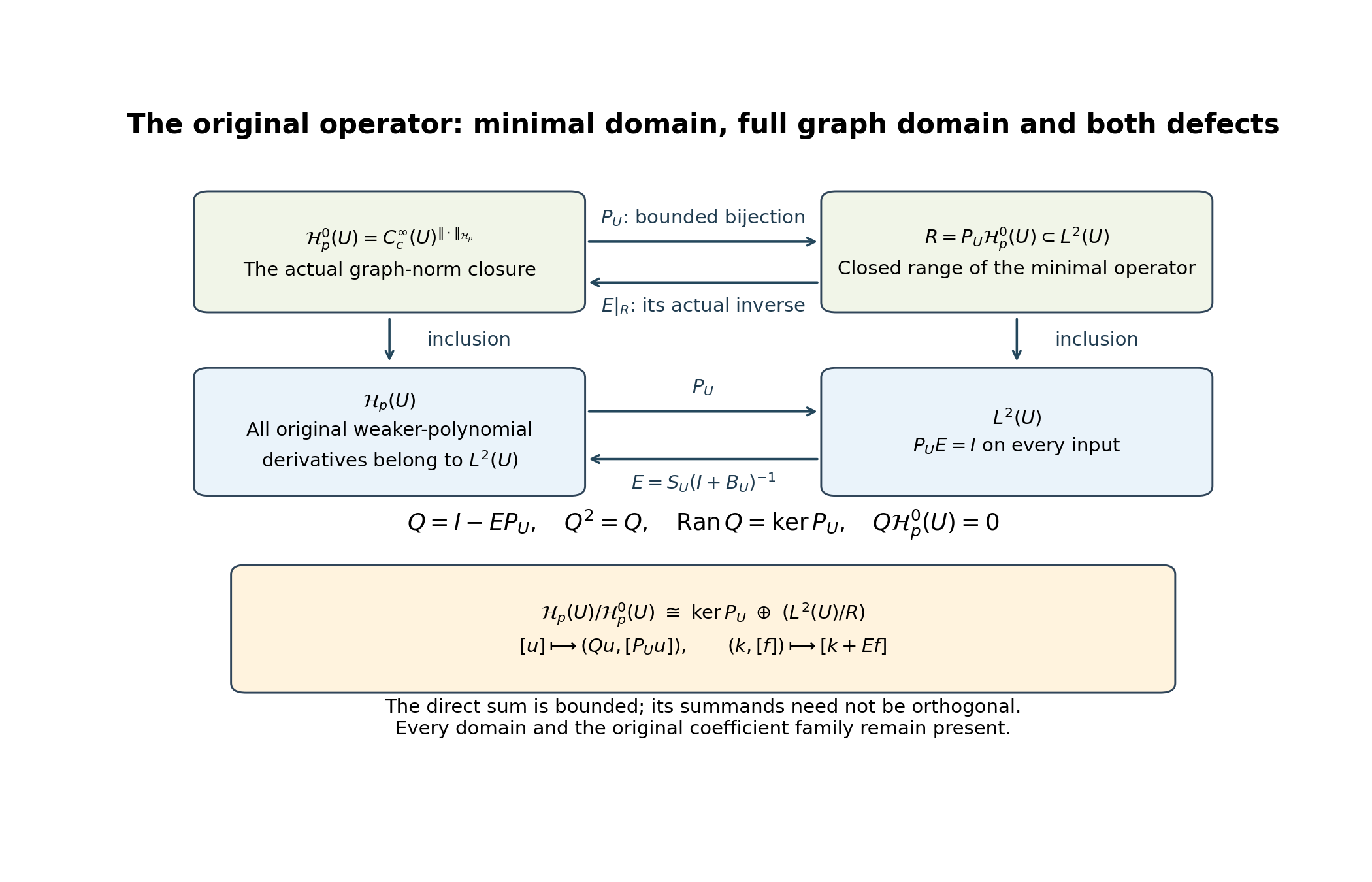
The accompanying figures retain the original graph spaces, coefficient, constants, and square. The first shows the maps of GM-A and GM-B, including the two opposite inverse arrows on the minimal domain and its actual closed image. Its notation means exactly the space in (GM7), and its means exactly . The displayed direct sum is topological; orthogonality in the original graph metric is not asserted. Its proof locators are (GM8)–(GM11) and (GM16)–(GM20).
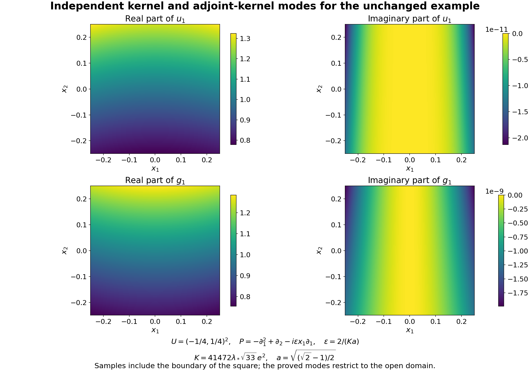
The second figure uses the exact mode from (GM34), and the exact adjoint mode
Indeed substitution of into (GM34) changes each product factor to , and substitution into (GM42) gives the exponential . Thus (GM38) proves , and (GM43), with every adjoint term retained, proves . These are two different operators and two explicitly specified modes.
The renderer retains terms , evaluates the coefficients with 80 decimal digits, and converts them to numerical display samples. The following bounds concern only the omitted exact series terms. They do not certify the numerical display rounding.
First the actual constants prove without numerical approximations. The orthonormal eigenbasis used here is proved in Fourier transforms, finite spectra and convex separation, Theorem3.1. For the real symmetric matrix in (GM29), its largest eigenvalue is at least its second diagonal entry : writing a unit vector in an orthonormal eigenbasis makes its quadratic form a weighted average of the eigenvalues, and the second coordinate vector has quadratic form . Since , one has . Also , since , so and . Therefore
For , each factor satisfies The complete product of these bounds is Thus on the closed original square, the -th series term after multiplication by has magnitude at most . For and an integer , The inequality holds because , including the empty product. Write for the sum of precisely the retained terms, including its exponential. The resulting bound is
For , the full adjoint factor obeys Its complete -fold product is at most . The bound proved in GM-D2 consequently bounds the coefficient by . On , the power contribution is at most . With defined using exactly the same retained indices,
The plotted grid includes the boundary of the square only to display these entire functions. Their graph-domain restrictions and all operator assertions use the unchanged open square . The retained renderer, formula record, image hashes, and actual visual-inspection records accompany this note. The pictures illustrate the proved maps and modes; the complete proofs above establish them.
9. The exact boundary realization on the original square
For the example, the graph closure in (GM7) can be characterized by actual traces without changing its norm or replacing its open square. Put , whose length is . The definition (GM32), with Fubini’s theorem, gives as functions in the first coordinate, and as such functions in the second coordinate. The weak derivative assertions are Hilbert-valued assertions: test first against products of two compactly supported smooth scalar functions, then use density of those functions in the other space and Cauchy–Schwarz to extend the equality to every fixed vector of that Hilbert space.
Here is the trace fact being used, including its proof. If , where is a Hilbert space, and the distributional derivative of is , then for a uniquely determined continuous, absolutely continuous representative on the closed interval. To see this, the Bochner integral is absolutely continuous and has weak derivative , as follows by scalar integration by parts after pairing with any vector of . Thus has distributional derivative zero. Every scalar test function of integral zero is the derivative of a compactly supported smooth function on . The derivative-zero identity consequently gives . Fix a scalar compactly supported smooth of integral one and subtract from any other test function; it follows that is the constant vector , as an -valued distribution and hence almost everywhere as an function. This proves (GM53). The integral formula is continuous on the closed interval by Cauchy–Schwarz and proves absolute continuity. Two continuous representatives equal almost everywhere are equal everywhere, which proves uniqueness.
Average over , where . The triangle inequality and Cauchy–Schwarz give the same bound at both endpoints: Apply this to and to in the first coordinate, and to in the second. This defines the six bounded trace maps all valued in the other space. The first bound uses the separate and terms of (GM32), the derivative trace bound uses , and the last uses . Since each unit factor in has modulus one, these are bounded for the exact original graph norm.
Theorem GM-F. The actual minimal domain for the unchanged example is exactly Consequently in GM-A1 is the realization of (GM30) on these six trace conditions. Its adjoint has exactly the distributional domain (GM26), with expression (GM41); no extra boundary trace condition is imposed on that adjoint domain.
Proof. Every compactly supported smooth function has all six zero traces. The bounds just proved show that their graph closure has the same zero traces. This proves one inclusion.
For the converse, let have all displayed zero traces, and extend it by zero from to . The Hilbert-valued formula (GM53) gives integration by parts in each coordinate, including the two endpoint values, by integrating the derivative of the scalar pairing. The zero terms remove the two boundary contributions for the first derivative. Applying that formula once more to , its zero terms remove the second pair. The zero terms remove the boundary contributions in the second coordinate. Tests with tensor products, then finite sums of them and their limits on compact sets, give the distributional identities on One can avoid the tensor approximation in this last step by pairing the Hilbert-valued integration-by-parts formula with the smooth -valued function supplied by an arbitrary two-variable test function. The scalar product rule follows from (GM53) and the ordinary derivative of that smooth function. Thus these equalities hold for every compactly supported smooth test, and every derivative on the right is . The full original graph norm of on is exactly that of on , with its two separate contributions.
For , define . This auxiliary approximation keeps both original coordinates in the receiving domain. Its support lies in , a distance from the boundary of . Distributional differentiation and the change of variables give, with every factor retained, The norm in this formula is the original sum on the indicated support; it is not an imposed rescaled norm.
For any , in as . Indeed for a compactly supported smooth function this follows by uniform convergence on a fixed compact support and dominated convergence. Such functions are dense in , by truncation and mollification as proved in GM-A1, and the dilation operator has exact norm , by its two-dimensional Jacobian. The approximation error is therefore bounded uniformly near , which proves the assertion for every . Apply it separately to , keeping the multipliers , to obtain in the original full graph norm.
Now convolve with a compactly supported smooth mollifier of integral one and radius . The result belongs to . Its constant-polynomial derivatives are the corresponding convolutions of : this follows by testing the convolution against a compactly supported smooth function and applying the definition of the distributional derivative. Each convolution tends to its input as . To prove that convergence directly, express its difference as the integral of translated differences of the input and apply the triangle inequality; translation continuity follows first for compactly supported smooth functions and then for all functions by their density and the exact unit norm of translation. Thus it also converges in the original graph sum. Choose and then a radius giving graph error below from . The resulting compactly supported smooth functions converge to in . This proves the converse inclusion and (GM56).
The identification of the closed minimal realization now follows from GM-A1. Its adjoint-domain assertion follows from the two inclusions proved for (GM26), with (GM41) as the actual expression. In particular the adjoint’s lack of an imposed trace condition is proved by that distributional-domain equality, rather than assumed from a formal integration-by-parts calculation. ∎
10. All bounded solver choices compatible with the minimal inverse
Write for the actual quotient map of (GM14), and for bounded linear maps between the indicated original normed spaces. Its operator norm uses those norms. Let These are exactly the bounded solvers that preserve both proved identities on their actual domains.
Theorem GM-G. The following is an affine bijection, with unique bounded parameters: Here retains the original norm. The affine bijection is isometric on differences: Its full operator-norm comparisons include The restricted-map norm is zero when . The original neighborhood is nonempty, so ; then proves . Before these estimates, the exact norm is No orthogonality between and is used to replace this formula by another norm.
Proof. If , then has image in ; hence . For , , so , and . Boundedness follows from the triangle inequality, , and the bound for .
Conversely let , and put . Since , , so . For every , choose with . Then . Define . The zero restriction to proves that this is well defined, and it is linear. For every , Taking the infimum proves and hence . The reverse bound follows from and the quotient inequality. Thus . Surjectivity of proves uniqueness of . Apply the same argument to to prove the displayed isometry on differences.
The first three triangle bounds in (GM59) now follow from and . In addition , so . For any nonzero , gives , proving . Finally , by the same minimal-domain argument used to prove , which proves the remaining lower bound. ∎
By the isometry in GM-C, this solver-parameter space is also exactly : if is bounded, the associated solver is ; conversely and . These formulas are inverse because and , and their operator norms agree because the quotient identification is an isometry. Thus the two proved defects determine the complete space of compatible choices, rather than only the failure of uniqueness.
For explicit choices in the unchanged example, define the adjoint modes using their actual exponent: The parameter conversion is written explicitly; at it gives exactly the retained of (GM49). The entire-function, full-domain, and independence proofs for apply under this bijective parameter conversion. In particular and .
For every , keep the exact rank-one correction The second formula is well defined because . Cauchy–Schwarz proves boundedness and the bounds by the product of the two original norms. Taking achieves the first bound. Its quotient class has norm one because , so the second bound is achieved as well. Thus their exact operator norms are All constituent norms, with every original graph contribution retained, are Both are finite by the complete compact derivative proofs above and positive because the modes have value one at the origin. In these exact integrals the exponential factor, including its exceptional real-part-zero case, is This follows by integrating at the two unchanged endpoints, or by integrating the constant one in the second case.
For a fully explicit finite bound in the same constants, put Equations (GM35) and (GM40) give Indeed by the actual area , and the square root of (GM40) gives times the displayed square root. This is a bound on the exact norm (GM62), rather than a replacement of its terms.
For any , the actual solver therefore satisfies both and on . Alternatively check the two corrections directly: because , and for because . Its norm is at most , and its distance from in operator norm is exactly , by (GM59). Distinct give distinct solvers since the correction is nonzero.
There are arbitrary finite independent grids of these corrections. To prove this completely, take distinct and distinct . The mode proofs give independent vectors and . The -by- matrix with entries is invertible: if a row combination of its rows were zero, the corresponding linear combination of the ’s would be orthogonal to each , hence to itself, and thus would be zero; independence then makes every row coefficient zero. Solving this exact finite matrix system gives vectors in their span with . If , apply it to to obtain . Independence of the ’s gives every . Thus all operators are independent. Taking and their diagonal sum gives a correction of exact rank : its image is contained in the span of the , and the test vectors map to those independent vectors. Every one of these finite-rank corrections belongs to the full parameter space (GM58).
The classification is a consequence of the two completed identities and the exact quotient maps, and its explicit variations use the two previously proved mode spaces. No classification of unbounded solvers, no additional regularity of all kernel elements, and no novelty assertion is made.
11. Literature comparison and the extent of the consequence
The comparison covers bounded passages of two freely accessible original-author TeX sources. The following locators identify the arguments actually compared; neither work supplies a new theorem as a premise for the domain and defect calculations proved here.
- Klaus Kröncke and Boris Vertman, Perelman’s Entropies for Manifolds with conical Singularities, arXiv:1902.02097: author TeX lines 934–1062, including the maximal/minimal/Friedrichs domain definitions, Proposition labelled minimal-domain-1 and its complete proof, and only the opening of the following corollary. The proposition concerns a conical Laplacian with link dimension at least three and its self-adjoint domain coincidence. The present square, full weaker-polynomial graph space, nonselfadjoint operator, nonzero drift, and two infinite-dimensional defect spaces are different specified objects. None of that source’s domain coincidence or parametrix conclusions is imported here.
- Robin J. Deeley, Magnus Goffeng, and Bram Mesland, The bordism group of unbounded KK-cycles, arXiv:1503.07398: author TeX lines 644–666, Lemma labelled firstgammadef and the following remark. That passage uses minimal Dirac domains and their adjoint maximal domains in a bundle setting. Here (GM26) is proved from the actual U006 expression and its graph closure, including continuous coefficients; no Dirac Sobolev-domain assertion is transferred.
The cited arXiv records identify the works. The comparison covers the passages specified above, rather than both complete works, and does not establish an identical arXiv source version. The projection and quotient argument is an elementary consequence of the completed two-sided identities on their actual domains. The explicit modes and adjoint modes are derived here from the unchanged operator, with their convergence and domain membership proved above.
The lesson’s statement that the construction supplies no uniqueness among all local solutions remains correct. Equations (GM11)–(GM12), (GM16)–(GM24), and the two mode families give its strongest domain relation established in this note: the completed inverse selects the closed complement , it inverts the injective minimal operator exactly on its closed image , and the full quotient has separate original kernel and adjoint-obstruction coordinates. These are editorial consequences linked to (CS40)–(CS50) and (CE25)–(CE34); no source passage is rewritten.