Alternation and the index under linear phase changes

Written and dedicated to the public domain by Codex, September 2026 (CC0).

For matrix symbols, reversing an ordered product is different from changing the sign of an exterior trace. We first prove the graded trace identity and expand the full alternating matrix word in the original phase coordinates. We then follow an actual symbol through an invertible real linear change, preserving its metric class and exterior inverse, and determine precisely how its analytic index changes. The result uses the original matrix index formula with its complete coefficient and outward orientation.

Read The matrix Weyl index in the original phase coordinates for the all-dimensional theorem (MB10), Scaled Weyl parametrices and the surviving differential degree for the original analytic Fredholm construction, Metric operator bounds for operator-norm continuity, and Relative Weyl projectors and the Chern cutoff form for the full matrix exterior and cutoff setting. From ordered Weyl errors to the exterior index form, equations (5)–(18), gives the independent direct proof from the same ordered errors.

1. Ordered exterior products and graded cyclic trace

Let $\alpha$ and $\beta$ be matrix-valued differential forms of degrees $p$ and $q$. Their exterior product wedges scalar form components and multiplies matrices in the written order. Expanding in elementary forms and using the finite matrix identity $\operatorname{tr}(UV)=\operatorname{tr}(VU)$ gives $$\operatorname{Tr}(\alpha\wedge\beta) =(-1)^{pq}\operatorname{Tr}(\beta\wedge\alpha). \tag{EF1}$$ This is a statement after matrix trace; the untraced products generally differ. In particular, for one-forms $\alpha,\beta$, rotate the first factor of the $2n$-fold ordered word $(\alpha\wedge\beta)^n$ past the remaining $2n-1$ one-forms. Its sign is $-1$, so $$\operatorname{Tr}[(\alpha\wedge\beta)^n] =-\operatorname{Tr}[(\beta\wedge\alpha)^n]. \tag{EF2}$$ Taking $\alpha=db,\beta=da$ proves the trace relation needed for the two parametrix orders without interchanging any untraced matrix factors.

To see the full orientation coefficient, put $z_{2j-1}=x_j,z_{2j}=\xi_j$ and $\Omega=dz_1\wedge\cdots\wedge dz_{2n}$. Directly expanding every wedge gives $$\operatorname{Tr}[(db\wedge da)^n] =\left[ \sum_{\sigma\in S_{2n}}\operatorname{sgn}(\sigma)\, \operatorname{tr}\!\left( \prod_{r=1}^{n} \bigl[(\partial_{z_{\sigma(2r-1)}}b) (\partial_{z_{\sigma(2r)}}a)\bigr]\right) \right]\Omega . \tag{EF3}$$ The product over $r$ is ordered from $1$ to $n$. Every permutation appears once, with its actual sign; no scalar determinant replaces the matrix word. For $n=1$, its coefficient is $\operatorname{tr}(b_xa_\xi-b_\xi a_x)$, the negative of the stated matrix Poisson bracket convention.

The matrix Poisson bracket itself is not generally antisymmetric before trace: $$\{b,a\} =\sum_j(b_{\xi_j}a_{x_j}-b_{x_j}a_{\xi_j}), \qquad \{a,b\} =\sum_j(a_{\xi_j}b_{x_j}-a_{x_j}b_{\xi_j}). \tag{EF4}$$ For a compactly supported example in dimension one, choose a smooth cutoff $\rho$ equal to one near $(0,0)$, $A=E_{12}$, $D=E_{21}$, $a=\rho xA$, and $b=\rho\xi D$. At the origin, $\{b,a\}=DA=E_{22}$ and $\{a,b\}=-AD=-E_{11}$. Their sum $E_{22}-E_{11}\ne0$. This example proves why the exact alternating trace of exterior words in (EF2) cannot be replaced by pointwise scalar antisymmetry.

2. The original isotropic symbol under a fixed linear map

Keep $g_z=(1+|z|^2)^{-1}|dz|^2$ on $\mathbb R^{2n}$ and $a\in S(1,g;\operatorname{End}\mathbb C^\nu)$, uniformly invertible outside a ball. If $T\in GL(2n,\mathbb R)$, define the actual transformed symbol $a_T(z)=a(Tz)$, with no replacement of its matrix values. For every derivative order $k$, the linear chain rule writes $D^k a_T(z)$ as a finite sum of $D^k a(Tz)$ applied to $T$-images of the $k$ directions. Since $\langle Tz\rangle\asymp_T\langle z\rangle$, the defining seminorms give $$a_T\in S(1,g),\qquad \|D^k a_T(z)\| \le C_{T,k}\langle z\rangle^{-k}. \tag{LS1}$$ If $a(w)$ is invertible for $|w|\ge R$, then $a_T(z)$ is invertible for $|z|\ge\|T^{-1}\|R$, with the same bound on its pointwise inverse. The proved scaled-parametrix result IP14 therefore makes $a_T^w$ Fredholm for every $T\in GL(2n,\mathbb R)$.

3. Norm-continuous transport along one component

Let $T_t$, $0\le t\le1$, be a continuously differentiable path in $GL(2n,\mathbb R)$. Compactness of the parameter interval supplies common bounds for $T_t$, $T_t^{-1}$ and $\dot T_t$. Differentiating any order-$k$ spatial derivative of $a(T_tz)$ produces terms with $D^k a(T_tz)$ times one differentiated $T_t$ factor, and a term with $D^{k+1}a(T_tz)\dot T_tz$. The latter is bounded by $C\langle z\rangle^{-k-1}|z|$, so every term obeys the original $S(1,g)$ order-$k$ bound uniformly in $t$. The fundamental theorem of calculus therefore gives convergence in each fixed finite symbol seminorm as $t$ varies. B26 turns this into operator-norm continuity: $$t\longmapsto(a\circ T_t)^w \quad\text{is continuous in } \mathcal L(L^2(\mathbb R^n;\mathbb C^\nu)). \tag{LS2}$$ Every member is Fredholm by Section 2. Norm stability of the Fredholm index gives $$\operatorname{ind}(a\circ T_1)^w =\operatorname{ind}(a\circ T_0)^w . \tag{LS3}$$

For clarity, the component with positive determinant is path connected without invoking an index theorem. Write $T=QP$ with $P=(T^tT)^{1/2}$ positive definite and $Q=TP^{-1}\in SO(2n)$. The path $(1-s)I+sP$ stays positive definite. Every real special orthogonal matrix has an orthogonal decomposition into two-dimensional rotation planes and fixed $+1$ directions: complex nonreal eigenvalues occur in conjugate pairs, while the $-1$ eigenspace has even dimension because the determinant is $+1$, and can be paired into rotation planes of angle $\pi$. Decreasing each rotation angle continuously to zero gives a path in $SO(2n)$ from $Q$ to $I$. Concatenating these paths yields a path from $I$ to $T$ in $GL^+(2n,\mathbb R)$. Hence $$\det T>0 \quad\Longrightarrow\quad \operatorname{ind}(a\circ T)^w =\operatorname{ind}a^w . \tag{LS4}$$ This proves the positive-determinant half of the analytic assertion independently of any exterior formula.

4. The boundary functional under both determinant signs

On the invertibility region let $\theta_a=a^{-1}da$. The ordinary pullback chain rule retains the matrix factor order and gives $$(a\circ T)^{-1}d(a\circ T)=T^*\theta_a,\qquad \operatorname{Tr} [((a\circ T)^{-1}d(a\circ T))^{2n-1}] =T^*\operatorname{Tr}(\theta_a^{2n-1}). \tag{LS5}$$ The closed odd trace form used for the boundary comparison has a complete local proof. On the original invertibility region differentiate $a^{-1}a=I$. This gives $d(a^{-1})=-a^{-1}(da)a^{-1}$, so $$d\theta_a=-\theta_a^2,\qquad d(\theta_a^{\,2n-1}) =-\sum_{r=0}^{2n-2}(-1)^r\theta_a^{\,2n} =-\theta_a^{\,2n}. \tag{EF5}$$ The sum has $2n-1$ terms and its alternating sum is one. By EF1, rotating the first degree-one factor of the even word gives $\operatorname{Tr}(\theta_a^{2n})=-\operatorname{Tr}(\theta_a^{2n})$, hence $$d\,\operatorname{Tr}(\theta_a^{\,2n-1}) =-\operatorname{Tr}(\theta_a^{\,2n})=0. \tag{EF6}$$ Every matrix multiplication and differential form remains in its original order before taking the graded trace.

Choose a ball $B_R$ in the $z$ variables large enough that both its boundary and the boundary of $T(B_R)$ lie in the respective invertibility regions and $T(B_R)$ contains the original noninvertible compact set. Orient every boundary by the stipulated positive ambient form $\Omega=dx_1\wedge d\xi_1\wedge\cdots\wedge dx_n\wedge d\xi_n$. The boundary change-of-variables rule, obtained by applying the Jacobian sign to an outward-normal-first oriented frame, gives $$\int_{\partial B_R} T^*\operatorname{Tr}(\theta_a^{2n-1}) =\operatorname{sgn}(\det T) \int_{\partial T(B_R)} \operatorname{Tr}(\theta_a^{2n-1}). \tag{LS6}$$ EF6 proves this odd trace form is closed on the invertibility region. Apply Stokes to the region between $\partial T(B_R)$ and any sufficiently large enclosing sphere $\partial B_{R'}$; the outer and inner induced boundary orientations have opposite signs. Therefore the two integrals without the Jacobian factor agree. In particular the original boundary functional obeys $$\int_{\partial B_R} \operatorname{Tr} [((a\circ T)^{-1}d(a\circ T))^{2n-1}] =\operatorname{sgn}(\det T) \int_{\partial B_{R'}} \operatorname{Tr}[(a^{-1}da)^{2n-1}] . \tag{LS7}$$ This is an exact geometric sign statement for every dimension. It does not rely on equality between the boundary functional and the analytic index.

5. Direct checks in dimensions one and two

For $n=1$, equations (16), (18) and (19) of From ordered Weyl errors to the exterior index form directly prove the full analytic formula with the original $dx_1\wedge d\xi_1$ orientation: $\operatorname{ind}a^w=(2\pi i)^{-1} \int_{\partial B}\operatorname{Tr}(a^{-1}da)$. Apply that same proved formula to $a\circ T$, then use (LS7). This gives, for every $T\in GL(2,\mathbb R)$, $$\operatorname{ind}(a\circ T)^w =\operatorname{sgn}(\det T)\operatorname{ind}a^w \qquad(n=1). \tag{LS8}$$ For $n=2$, equations (16), (18), (20) and (21) of that same direct lesson evaluate the finite coefficient completely, with the original ambient orientation and the same analytic receiving map for $a$ and $a\circ T$. Apply that proved formula to both symbols, and then apply (LS7) to their odd boundary forms. The exact constant $1/(24\pi^2)$ is identical on both sides, so it factors out without a sign change. Thus $$\operatorname{ind}(a\circ T)^w =\operatorname{sgn}(\det T)\operatorname{ind}a^w \qquad(T\in GL(4,\mathbb R),\ n=2). \tag{LS9}$$ The dimension-one and dimension-two calculations independently check the all-dimensional argument that follows.

6. The all-dimensional analytic sign

MB10 proves for every $n\geq1$, every original $a\in S(1,g;\operatorname{End}\mathbb C^\nu)$ uniformly invertible outside a compact set, and the original $\Omega$-outward boundary orientation, $$\operatorname{ind}a^w =D_n\int_{\partial B}^{\Omega} \operatorname{Tr}[(a^{-1}da)^{2n-1}], \qquad D_n=-(-2\pi i)^{-n} \frac{(n-1)!}{(2n-1)!}. \tag{LS10}$$ This is the full coefficient, with its sign, $\pi$- and $i$-powers and factorials. LS1 proves that $a\circ T$ meets the same symbol and exterior-invertibility hypotheses for every $T\in GL(2n,\mathbb R)$; its matrix size and its $D_n$ are unchanged. Apply (LS10) to $a\circ T$, use the exact pullback identity (LS5) and the oriented boundary change (LS7), and then apply (LS10) back to $a$: $$\begin{aligned} \operatorname{ind}(a\circ T)^w &=D_n\int_{\partial B_R}^{\Omega} \operatorname{Tr} [((a\circ T)^{-1}d(a\circ T))^{2n-1}]\\ &=\operatorname{sgn}(\det T)\,D_n \int_{\partial B_{R'}}^{\Omega} \operatorname{Tr}[(a^{-1}da)^{2n-1}]\\ &=\operatorname{sgn}(\det T)\operatorname{ind}a^w, \qquad T\in GL(2n,\mathbb R),\quad n,\nu\geq1. \end{aligned} \tag{LS11}$$ There is no metaplectic or unitary-conjugacy assertion for a general $T$; the second line is the proved boundary pullback, and the first and last lines are separate applications of the proved original matrix index theorem. The analytic formula is therefore closed at precisely the hypotheses of MB10. The independent direct calculation in the exterior-reduction lesson, equations (5)–(18), proves the same analytic sign using the full finite ordered coefficient and its exterior evaluation.

7. Worked example: a reflection changes a nonzero index

Use the same full bounded one-plane symbol as (MI1), $$a(x,\xi)=\frac{x+i\xi}{\sqrt{1+x^2+\xi^2}}, \qquad T(x,\xi)=(-x,\xi),\qquad \det T=-1. \tag{LI1}$$ The symbol $a$ has index $+1$ by the proved formula (MB10), as calculated directly in (MI2). Both $a$ and $a\circ T$ belong to the original $S(1,g)$ class and have a uniformly bounded inverse outside a ball. On the positively oriented circle $(x,\xi)=R(\cos\vartheta,\sin\vartheta)$, the denominator is positive and $$(a\circ T)(R\cos\vartheta,R\sin\vartheta) =\frac{R e^{i(\pi-\vartheta)}}{\sqrt{1+R^2}}, \qquad (a\circ T)^{-1}d(a\circ T)=-i\,d\vartheta. \tag{LI2}$$ The original $n=1$ coefficient is $D_1=1/(2\pi i)$. Therefore $$\operatorname{ind}(a\circ T)^w =\frac1{2\pi i}\int_0^{2\pi}(-i)\,d\vartheta =-1 =\operatorname{sgn}(\det T)\operatorname{ind}a^w. \tag{LI3}$$ This checks an actual nonzero analytic sign change without treating the non-symplectic reflection as a unitary conjugation.

8. Exercises with solutions

Exercise 1. In two phase planes let $T$ change only $x_1$ to $-x_1$, leaving $\xi_1,x_2,\xi_2$ fixed. Determine the index of $(a\circ T)^w$ from $\operatorname{ind}a^w=m$, and calculate the coefficient $D_2$ separately.

Solution. In the original ordered coordinates $\det T=-1$. Equation (LS11) gives $\operatorname{ind}(a\circ T)^w=-m$, including for noncommutative matrix symbols. The complete coefficient is $$D_2=-(-2\pi i)^{-2}\frac{1!}{3!} =\frac{1}{24\pi^2}. \tag{LI4}$$ The minus sign of the transformed index comes from the boundary orientation in (LS7), not from changing $D_2$.

Exercise 2. Why does $\operatorname{Tr}[(db\wedge da)^n]=-\operatorname{Tr}[(da\wedge db)^n]$ not imply $\{b,a\}=-\{a,b\}$ as untraced matrices?

Solution. Equation (EF2) rotates one degree-one factor through $2n-1$ others inside a matrix trace, using graded cyclicity (EF1). It does not commute the matrix coefficients. In (EF4)’s exact compact two-by-two local example, $\{b,a\}=E_{22}$ and $\{a,b\}=-E_{11}$ at the origin, so their untraced sum $E_{22}-E_{11}$ is nonzero. The traced exterior assertion and the untraced Poisson assertion have different algebraic hypotheses.

9. References

• M. Pflaum, H. Posthuma and X. Tang, Cyclic cocycles on deformation quantizations and higher index theorems, arXiv:0805.1411v3, IndThms.tex, theorem thm:higher-algind and proof, lines 412–479. The preceding matrix-index lesson proves its specialization to the original symbols and all factor and orientation comparisons.

10. Every derivative in the linear transport

Here we supply the estimates and finite-dimensional constructions used in Sections 2–4. Keep the original ordered coordinates, the full matrix symbol and the actual map $T$. Write $d=2n$, $\langle z\rangle=(1+|z|^2)^{1/2}$, and, for this same symbol, set $$A_k(a)=\sup_z\langle z\rangle^k \|D^k a(z)\|_{(\mathbb R^d)^k\to\operatorname{End}\mathbb C^\nu}, \qquad p_{\le J}(a)=\sum_{k=0}^J A_k(a). \tag{LT1}$$ For $k=0$ the norm means the matrix norm itself. These are exactly the derivative norms for the original metric: $g_z(v)\le1$ means $|v|\le\langle z\rangle$, so the supremum of $\|D^ka(z)(v_1,\ldots,v_k)\|$ over the original metric unit vectors is $\langle z\rangle^k\|D^ka(z)\|$. They measure the unchanged $a$; no coordinate or symbol is being substituted for it. In particular each $A_k(a)$ is finite.

Let $$m_T=\|T^{-1}\|^{-1},\qquad \mu_T=\min(1,m_T),\qquad L_T=\max(1,\|T\|). \tag{LT2}$$ The inverse identity gives $|z|=|T^{-1}Tz|\le\|T^{-1}\||Tz|$, and the operator norm gives the upper bound. Adding the unchanged constant one proves both inequalities $$\mu_T^2(1+|z|^2)\le1+|Tz|^2 \le L_T^2(1+|z|^2). \tag{LT3}$$ The complete coordinate chain rule is $$\partial_{j_1}\cdots\partial_{j_k}a(Tz) =\sum_{\ell_1,\ldots,\ell_k=1}^d \left(\prod_{r=1}^k T_{\ell_rj_r}\right) (\partial_{\ell_1}\cdots\partial_{\ell_k}a)(Tz). \tag{LT4}$$ The product here consists of scalar entries; the matrix derivative remains intact. For $k=0$ the sum has its single empty term $a(Tz)$. The first-order formula follows by differentiating each coordinate of $Tz$. Induction differentiates only the last derivative, because every entry of $T$ is constant in $z$, and proves the displayed sum for every $k$.

Equivalently, applying that full sum to $v_1,\ldots,v_k$ gives $D^ka(Tz)(Tv_1,\ldots,Tv_k)$. Hence $$A_k(a\circ T)\le\|T\|^k\mu_T^{-k}A_k(a). \tag{LT5}$$ All constants and the original $1+|z|^2$ are retained in (LT3)–(LT5). If coordinate derivative norms are used instead, expanding the same multilinear form gives their comparison explicitly. With $M_k$ the maximum of the weighted norms of its coordinate derivatives, $$M_k(a)\le A_k(a)\le d^{k/2}M_k(a). \tag{LT6}$$ Indeed the expansion has all $d^k$ terms, and its norm is bounded by $M_k\prod_r\sum_j|v_{rj}|$. Cauchy–Schwarz gives $\sum_j|v_{rj}|\le\sqrt d\,|v_r|$. The other inequality evaluates the multilinear form on coordinate unit vectors. Thus either of these finite seminorm lists gives the exact continuity required by B26.

Now let $T_t$ be the original continuously differentiable path. The full derivative of (LT4), including every matrix-entry derivative and every coordinate of $\dot T_tz$, is $$\begin{aligned} &\partial_t\partial_{j_1}\cdots\partial_{j_k}a(T_tz)\\ &=\sum_{\ell_1,\ldots,\ell_k=1}^d \sum_{s=1}^k (\dot T_t)_{\ell_sj_s} \left(\prod_{\substack{1\le r\le k\\r\ne s}} (T_t)_{\ell_rj_r}\right) (\partial_{\ell_1}\cdots\partial_{\ell_k}a)(T_tz)\\ &\quad+\sum_{\ell_1,\ldots,\ell_k=1}^d \left(\prod_{r=1}^k(T_t)_{\ell_rj_r}\right) \sum_{q,p=1}^d(\dot T_t)_{qp}z_p (\partial_q\partial_{\ell_1}\cdots\partial_{\ell_k}a)(T_tz). \end{aligned} \tag{LT7}$$ For $k=0$ the first sum is empty, and the second is $\sum_{q,p}(\dot T_t)_{qp}z_p\partial_qa(T_tz)$. This accounts for the term that would be lost by differentiating only the prefactor.

Put $L=\sup_t\|T_t\|$, $H=\sup_t\|\dot T_t\|$, and $\mu=\min(1,\inf_t\|T_t^{-1}\|^{-1})$. The inverse entries are the signed minor polynomials divided by the nonzero determinant; they are continuous. On the compact interval the norms are bounded, so $L>0$, $H<\infty$ and $\mu>0$. In multilinear notation the first sum in (LT7) has $k$ terms with one $\dot T_t$ and $k-1$ copies of $T_t$. The second has $k$ copies of $T_t$ and the extra argument $\dot T_tz$. Using (LT3) for this common $\mu$ yields $$A_k\bigl(\partial_t(a\circ T_t)\bigr) \le H\left[kL^{k-1}\mu^{-k}A_k(a) +L^k\mu^{-k-1}A_{k+1}(a)\right]. \tag{LT8}$$ At $k=0$ omit the first term. In the last term the retained factor is $|z|/\langle z\rangle\le1$. The finite-dimensional fundamental theorem of calculus, applied to every matrix entry and derivative, gives $$A_k(a\circ T_t-a\circ T_u) \le |t-u|H\left[kL^{k-1}\mu^{-k}A_k(a) +L^k\mu^{-k-1}A_{k+1}(a)\right]. \tag{LT9}$$ The common bound permits the supremum in $z$ and unit directions after integration. Summing through the actual finite $J$ of B26 proves (LS2), with every spatial derivative and parameter derivative accounted for.

There is a stronger continuity statement. Fix $T\in GL(d,\mathbb R)$ and take $S$ with $\|S-T\|<m_T/2$. Along the actual segment $T_s=T+s(S-T)$, $$|T_sz|\ge(m_T-\|S-T\|)|z|\ge(m_T/2)|z|, \qquad\|T_s\|\le\|T\|+m_T/2. \tag{LT10}$$ The lower bound makes every $T_s$ injective, hence invertible in this finite dimension. Use $\mu=\min(1,m_T/2)$, $L=\|T\|+m_T/2$ and $H=\|S-T\|$ in (LT9). It proves $$A_k(a\circ S-a\circ T) \le\|S-T\|\left[kL^{k-1}\mu^{-k}A_k(a) +L^k\mu^{-k-1}A_{k+1}(a)\right]. \tag{LT11}$$ Thus $T\mapsto a\circ T$ is locally Lipschitz in every fixed original symbol seminorm. B26 proves local Lipschitz continuity of $T\mapsto(a\circ T)^w$ in operator norm. Every continuous path $T_t$ consequently gives a continuous operator path; differentiability of the path is unnecessary. Section 2 and IP14 still prove Fredholmness at every parameter. The norm-stability proof in Section 3 of Finite defects under perturbation makes its index locally constant. A locally constant integer on $[0,1]$ is constant: if two values occurred, the set of points reached from zero with its value and its open complement would separate the interval; taking the supremum of an initial interval of that value contradicts local constancy at its endpoint. This proves (LS3) for all continuous paths, while retaining the original differentiable-path calculation (LT7)–(LT9).

11. The full positive square root and orthogonal rotation planes

We prove the original polar and orthogonal-plane assertions. First consider any real symmetric $d$-by-$d$ matrix $H$. Its quadratic form has a maximum on the unit sphere. Here is the finite compactness fact needed for this statement. A bounded real sequence has a convergent subsequence: bisect a containing closed interval, keep a half containing infinitely many terms, repeat, and choose increasing sequence indices from those halves. The nested lengths tend to zero; the chosen values converge to their common endpoint limit. Repeating for each of the finitely many coordinates yields a convergent subsequence of any bounded sequence in $\mathbb R^d$. The unit sphere is closed because the sum of coordinate squares is continuous. A maximizing sequence for the bounded continuous quadratic form therefore has a sphere subsequence whose limit attains its supremum. Its boundedness follows from the finite sum $\sum_{j,k}|H_{jk}||v_j||v_k|$ for $|v|=1$.

Let $v$ be such a maximizing unit vector and $u\perp v$. On the unit curve $(v+tu)/(1+t^2|u|^2)^{1/2}$, the derivative of the quadratic form at zero is $2\langle u,Hv\rangle$; it must vanish. Thus $Hv=\lambda v$. Symmetry gives $\langle v,Hu\rangle=\langle Hv,u\rangle=0$, so $v^\perp$ is invariant. Induction on its dimension gives an orthonormal eigenbasis $v_1,\ldots,v_d$, with $$H=\sum_{j=1}^d\lambda_j v_jv_j^t. \tag{LP1}$$ All eigenvalues and all orthogonal projections are retained. For the original $H=T^tT$, $$\lambda_j=\langle v_j,T^tTv_j\rangle=|Tv_j|^2>0, \qquad P=\sum_{j=1}^d\sqrt{\lambda_j}\,v_jv_j^t, \quad P^{-1}=\sum_{j=1}^d\lambda_j^{-1/2}v_jv_j^t. \tag{LP2}$$ Orthogonality of the projections proves $P^2=T^tT$, $PP^{-1}=I$, and positive definiteness of $P$. This positive symmetric square root is unique. If $W$ is another such root, then $WH=HW$, since $H=W^2$; it preserves each eigenspace of $H$. Apply (LP1) to its symmetric restriction there. Every positive eigenvalue $r$ of $W$ satisfies $r^2=\lambda$, so that restriction is $\sqrt\lambda I$. Hence $W=P$.

Set $Q=TP^{-1}$, exactly as in Section 3. Direct multiplication proves $$Q^tQ=P^{-1}T^tTP^{-1}=I, \qquad T=QP, \qquad \det P=\prod_{j=1}^d\sqrt{\lambda_j}>0, \qquad\det Q=\frac{\det T}{\prod_j\sqrt{\lambda_j}}. \tag{LP3}$$ An orthogonal matrix has determinant $+1$ or $-1$, since taking determinants in $Q^tQ=I$ gives $(\det Q)^2=1$. Thus its determinant is precisely the sign of the original $\det T$. The original positive-definite path also follows without deleting any eigenspace: $$(1-s)I+sP =\sum_{j=1}^d(1-s+s\sqrt{\lambda_j})v_jv_j^t, \qquad 0\le s\le1. \tag{LP4}$$ Every coefficient is positive, including at both endpoints.

For the rotation-plane assertion, start with this same real orthogonal $Q$ and retain both its parts $$C=\tfrac12(Q+Q^t),\qquad K=\tfrac12(Q-Q^t), \qquad C^t=C,\quad K^t=-K. \tag{LP5}$$ Since $QQ^t=Q^tQ=I$, expanding both products gives $$CK=KC,\qquad C^2-K^2=I, \qquad Q=C+K. \tag{LP6}$$ By (LP1), $C$ has mutually orthogonal real eigenspaces $E_c$. Commutation shows $K(E_c)\subset E_c$. On that actual space, $$K^2=(c^2-1)I, \qquad |Kv|^2=-\langle v,K^2v\rangle=(1-c^2)|v|^2. \tag{LP7}$$ Therefore $|c|\le1$. If $c=1$ or $c=-1$, the right side is zero, so $K=0$ there and $Q=I$ or $Q=-I$, respectively. If $-1<c<1$, put $\sigma=(1-c^2)^{1/2}>0$. Choose a unit $v\in E_c$ and put $w=Kv/\sigma$. Skew symmetry gives $\langle v,w\rangle=0$; (LP7) gives $|w|=1$. The full action on this plane is $$Kv=\sigma w,\quad Kw=-\sigma v, \qquad Qv=cv+\sigma w,\quad Qw=-\sigma v+cw. \tag{LP8}$$ Its orthogonal complement inside $E_c$ is invariant under $K$, because inner products of $Ku$ with $v,w$ equal the negatives of the inner products of $u$ with $Kv,Kw$. Repeating decomposes all of $E_c$ into these two-dimensional planes. Each plane has the exact matrix $$R(c,\sigma)=\begin{pmatrix}c&-\sigma\\\sigma&c\end{pmatrix}, \qquad c^2+\sigma^2=1,\quad\det R=1. \tag{LP9}$$ The remaining spaces are fixed $+1$ directions and $-1$ directions. The determinant of $Q$ is the product of their signs and the plane determinants. When $\det Q=1$, the number of $-1$ directions is even, and pairing them gives planes $R(-1,0)$. This proves the exact decomposition claimed earlier. Its complex eigenvalues on each nonreal plane are the conjugate roots $c+i\sigma,c-i\sigma$ of $\lambda^2-2c\lambda+1$; the $-1$ and $+1$ cases were proved over the reals as well.

We also construct every needed path explicitly. If $(c,\sigma)\ne(-1,0)$, define $$(c_s,\sigma_s)= \frac{(1-s+sc,\,s\sigma)} {\sqrt{(1-s+sc)^2+s^2\sigma^2}},\qquad 0\le s\le1. \tag{LP10}$$ The denominator can vanish only if $s\sigma=0$ and $1-s+sc=0$. At $s=0$ the second expression is one. If $s>0$, these two equalities force $\sigma=0,c=-1,s=1/2$, which was excluded. Thus (LP10) is a smooth path of actual unit pairs from $(1,0)$ to $(c,\sigma)$. For $(-1,0)$, use first the same normalized segment from $(1,0)$ to $(0,1)$, then the segment from $(0,1)$ to $(-1,0)$. Neither segment has opposite endpoints, so the same nonvanishing proof applies. Every matrix $R(c_s,\sigma_s)$ is real orthogonal with determinant one.

Choose the actual orthonormal basis of all these planes and fixed directions, and call its change-of-basis matrix $O$. Conjugating the block paths by $O$ gives a continuous, piecewise smooth $Q_s\in SO(d)$ with $Q_0=I,Q_1=Q$. No eigenvalue, direction or plane is discarded. The exact concatenated path from the identity to the original $T$ is $$T_s=\begin{cases} Q_{2s},&0\le s\le\tfrac12,\\ Q\bigl((2-2s)I+(2s-1)P\bigr),&\tfrac12\le s\le1. \end{cases} \tag{LP11}$$ Its endpoints are $I,T$, the two formulas agree at $s=1/2$, and their determinants are positive by (LP4) and $\det Q=1$. Equations (LT10)–(LT11) and Fredholm stability apply to this continuous path, proving (LS4) with all its prerequisites supplied.

For completeness these are exactly the two path components of $GL(d,\mathbb R)$. A continuous determinant cannot pass between its signs without zero, by the intermediate value theorem. The positive component is connected by (LP11). For a negative-determinant $T$, retain $J=\operatorname{diag}(-1,1,\ldots,1)$. The matrix $JT$ has positive determinant; multiplying its identity-to-$JT$ path on the left by this same $J$ gives a negative-determinant path from $J$ to $T$. This proves connectedness of that component. The analytic index of $(a\circ T)^w$ is consequently constant on each component for the unchanged $a$, by (LS3).

12. The oriented boundary comparison with a global primitive

We give the complete integration argument for (LS6)–(LS7). It also proves a geometric strengthening: these two boundary identities hold for any smooth $\nu$-by-$\nu$ matrix $a$ on $\mathbb R^{2n}$ that is invertible outside a compact set. Neither symbol estimates nor a uniform bound on the exterior inverse is needed for this geometric assertion. The analytic Fredholm results continue to use their original symbol and inverse bounds.

Choose $\rho>0$ so that the noninvertible set lies in $B_\rho$. A smooth admissible cutoff can be constructed explicitly. Set $\eta(t)=e^{-1/t}$ for $t>0$ and $\eta(t)=0$ for $t\le0$, and $$\chi(t)=\frac{\eta(t)}{\eta(t)+\eta(1-t)},\qquad \psi(z)=\chi\!\left(\frac{|z|^2-\rho^2}{3\rho^2}\right). \tag{LG1}$$ Every derivative of $\eta$ on $t>0$ is $e^{-1/t}$ times a finite polynomial in $t^{-1}$. Each tends to zero at the origin: with $u=1/t$, the inequality $e^u\ge u^N/N!$, taking $N$ greater than each polynomial degree, proves this limit. Induction therefore proves that the zero extension is smooth. The denominator in $\chi$ is positive everywhere, since $t\le0$ and $1-t\le0$ cannot both hold. Thus $\psi$ is smooth, is zero on $\overline{B_\rho}$, and is one for $|z|\ge2\rho$. In particular $K=\operatorname{supp}(1-\psi)=\overline{B_{2\rho}}$, and every possible noninvertible point has a neighborhood where $\psi=0$.

On the actual invertibility region $U_a$, keep $$\theta=a^{-1}da,\quad\omega=\operatorname{Tr}(\theta^{2n-1}), \qquad F_n(t)=n\int_0^t u^{n-1}(1-u)^n\,du =n\sum_{j=0}^n(-1)^j\binom nj\frac{t^{n+j}}{n+j}. \tag{LG2}$$ Equations (EF1), (EF5) and (EF6) prove $d\omega=0$, with all matrix orders retained. Define $\beta=F_n(\psi)\omega$ on $U_a$, extending it by zero near the noninvertible set. It is globally smooth: $F_n(0)=0$, and $\psi$ is identically zero on that whole neighborhood. The complete product differentiation gives $$\begin{aligned} d\beta &=n\psi^{n-1}(1-\psi)^n d\psi\wedge\omega +F_n(\psi)d\omega\\ &=n\psi^{n-1}(1-\psi)^n d\psi\wedge\omega,\\ F_n(1)&=n\int_0^1u^{n-1}(1-u)^n\,du =\frac{n\,(n-1)!\,n!}{(2n)!} =\frac{(n!)^2}{(2n)!}>0. \end{aligned} \tag{LG3}$$ The first term extends by zero in the same manner. Its support is contained in the original compact $K$, since $d\psi=0$ where $\psi=1$. The full factorial moment is proved by repeated one-dimensional integration by parts in ES4 of Relative Weyl projectors and the Chern cutoff form. Its positivity also follows directly from its strictly positive integrand on $0<u<1$. Equation (LG3) is the same global primitive as BN2–BN3, with all its factors intact.

We first justify the exact distinction between the signed determinant and the absolute determinant in integration. For any compactly supported smooth complex function $f$ on $\mathbb R^d$ and any real invertible $T$, $$\int_{\mathbb R^d}f(Tz)\,dz =\frac1{|\det T|}\int_{\mathbb R^d}f(w)\,dw, \qquad T^*\Omega=(\det T)\Omega. \tag{LG4}$$ For the first equality it suffices to prove it for the exact elementary factors of $T$. Swapping two coordinates preserves the Lebesgue integral by Fubini and has determinant $-1$. Scaling one coordinate by $c\ne0$ gives the factor $1/|c|$ by the one-dimensional substitution formula; when $c<0$, reversing the integration endpoints supplies the absolute value. Adding $c$ times coordinate $k$ to a different coordinate $j$ preserves the integral: fix every other coordinate and translate the $j$-th line by the actual constant $cz_k$. Its determinant is one. The one-dimensional substitutions follow from the fundamental theorem of calculus applied to a compactly supported continuous integrand’s primitive. All the functions here are integrable, so Fubini applies to their real and imaginary parts.

Every invertible matrix is a finite product of these actual elementary factors. At each elimination stage its next column has a nonzero entry among the remaining rows; otherwise the remaining square block would have a zero column and determinant zero. Swap that entry into the pivot position, scale by its nonzero pivot inverse, and subtract its required multiples from the other rows. Continuing in the remaining block and then eliminating above the pivots produces the identity. Each reverse step is an elementary factor of the same type. Their determinants multiply, so applying their already proved substitutions successively gives the full $|\det T|^{-1}$ in (LG4). This is a proof concerning the original $T$, preserving its determinant and all its factors. The second equality in (LG4) follows by expanding the entire wedge $d(Tz)_1\wedge\cdots\wedge d(Tz)_d$: its coefficient is the full signed permutation sum defining $\det T$.

Let $\nu=z/R$ be the unit outward normal to $\partial B_R$, and set $w=Tz$. The ellipsoid $T(B_R)$ is defined by $|T^{-1}w|^2<R^2$. Differentiating this full quadratic defining function gives its unit outward normal and the full transverse factor $$\nu_w=\frac{T^{-t}\nu}{|T^{-t}\nu|},\qquad (T\nu)\cdot\nu_w=\frac1{|T^{-t}\nu|}>0. \tag{LG5}$$ Thus $T\nu$ is outward transverse, even though it generally differs from the Euclidean normal. If $(e_1,\ldots,e_{d-1})$ is a positive orthonormal tangent frame on the sphere, then the complete determinant identity gives $$\Omega(T\nu,Te_1,\ldots,Te_{d-1})=\det T, \qquad \Omega(\nu_w,Te_1,\ldots,Te_{d-1}) =|T^{-t}\nu|\det T. \tag{LG6}$$ To obtain the second equality, subtract from $T\nu$ its tangent component; wedge evaluation kills that component, while its remaining normal component is exactly (LG5). The absolute value of the second determinant is the tangential area factor $$J_{\partial T}(z)=|\det T|\,|T^{-t}\nu|. \tag{LG7}$$ Indeed the squared volume of a tangent parallelepiped equals its Gram determinant, by expanding its coordinates in any orthonormal basis of the tangent hyperplane. Adjoining the unit normal does not change that Gram determinant. This proves the area factor and the orientation sign simultaneously: the actual image tangent frame is positive precisely when $\det T>0$.

These frame identities prove the boundary substitution for any smooth $(d-1)$-form $\gamma$ on a neighborhood of the ellipsoid boundary. Use the finite sphere graph charts from the proof of ES6–ES7 in the relative-projector lesson. In a chart $z=z(u)$, the image chart is exactly $w=Tz(u)$, and pullback evaluation is $\gamma_w(T\partial_{u_1}z,\ldots,T\partial_{u_{d-1}}z)$. The image area is multiplied by (LG7); its orientation relative to the outward image normal has the sign given by (LG6). Integrating each chart, with a partition of unity transported by $T$, therefore proves $$\int_{\partial B_R}^{\Omega}T^*\gamma =\frac{\det T}{|\det T|} \int_{\partial T(B_R)}^{\Omega}\gamma. \tag{LG8}$$ There is no unstated sign from a normal replacement: its multiplier was proved positive in (LG5). A finite partition can be constructed by choosing smaller graph neighborhoods covering the compact sphere, taking smooth nonnegative coordinate cutoffs positive on those smaller neighborhoods, and dividing each by the positive sum. Coordinate cutoffs follow from the same $\eta$ construction in (LG1). Their transported sum is still one. Thus the chart sums give the full boundaries, including the overlaps. Applying (LG8) to $\gamma=\omega$ proves (LS6).

Finally choose actual radii $$R>2\rho\max(1,\|T^{-1}\|),\qquad R'>\max(2\rho,\|T\|R). \tag{LG9}$$ Then $K\subset B_R$, $K\subset T(B_R)$, and $T(B_R)\subset B_{R'}$, with collars of all relevant boundaries lying where $\psi=1$. Write the globally smooth compact derivative as $d\beta=V(w)\Omega$. Its pullback is the full top form $T^*d\beta=(\det T)V(Tz)\Omega$. The supports of $V$ and $V\circ T$ are inside $B_{R'}$ and $B_R$, respectively. Applying (LG4) to this actual compact $V$, with no interior inverse required, proves $$\begin{aligned} \int_{B_R}T^*d\beta &=\det T\int_{\mathbb R^d}V(Tz)\,dz\\ &=\frac{\det T}{|\det T|} \int_{\mathbb R^d}V(w)\,dw\\ &=\operatorname{sgn}(\det T)\int_{B_{R'}}d\beta. \end{aligned} \tag{LG10}$$ ES7 applies to the globally smooth forms $T^*\beta$ and $\beta$ on their two closed balls. The identity $d(T^*\beta)=T^*(d\beta)$ follows by differentiating their full finite coordinate expansions: all second derivatives of the linear map vanish, and the first-derivative factors are exactly those of the exterior pullback. The boundary values of the two primitives are $F_n(1)T^*\omega$ and $F_n(1)\omega$. Consequently (LG10) gives $$F_n(1)\int_{\partial B_R}^{\Omega}T^*\omega =\operatorname{sgn}(\det T)F_n(1) \int_{\partial B_{R'}}^{\Omega}\omega. \tag{LG11}$$ Retaining the nonzero full value $F_n(1)=(n!)^2/(2n)!$ before division proves (LS7). It also proves equality of the outward sphere and ellipsoid integrals appearing in Section 4, by (LS6). Every contribution through the noninvertible interior was carried by the globally smooth primitive; none was assigned an inverse there.

For the more general smooth exterior-invertible matrices stated at the start of this section, (EF5)–(EF6) are unchanged. The cutoff, the global primitive, all compact supports and both ball integrations remain valid. This proves that geometric extension at exactly its stated hypotheses. Equations (LT1)–(LT11) and IP14 separately supply the original analytic symbol and Fredholm hypotheses; the two scopes are identified by these explicit maps and computations.

13. An exact circle-to-ellipsoid orientation sample

The following sample depicts the geometry of (LG5)–(LG8). In the original one-plane coordinate order $(x_1,\xi_1)$, take the actual ball radius $2$ and the full auxiliary map $$T=\begin{pmatrix}-2&0\\0&\tfrac12\end{pmatrix},\qquad \det T=(-2)\tfrac12=-1,\qquad z(\vartheta)=(2\cos\vartheta,2\sin\vartheta), \quad Tz(\vartheta)=(-4\cos\vartheta,\sin\vartheta). \tag{LO1}$$ Its image boundary has the exact equation $w_1^2/16+w_2^2=1$. The image of the positive input path is clockwise: at $\vartheta=0$ it is at $(-4,0)$ with derivative $(0,1)$, directed upward at the left endpoint. The positively oriented ambient ellipse path is $(4\cos\varphi,\sin\varphi)$; at its same left endpoint $\varphi=\pi$, its derivative is $(0,-1)$. The exact relation $\varphi=\pi-\vartheta$ retains this sign on the full circle.

At $\vartheta=\pi/4$ the positive input normal and tangent are $\nu=(1,1)/\sqrt2$, $e=(-1,1)/\sqrt2$. All the factors in the image frame are $$\begin{aligned} T\nu&=(-\sqrt2,\sqrt2/4),& Te&=(\sqrt2,\sqrt2/4),\\ T^{-t}\nu&=(-\sqrt2/4,\sqrt2),& |T^{-t}\nu|&=\sqrt{34}/4,\\ \nu_w&=(-1,4)/\sqrt{17},& (T\nu)\cdot\nu_w&=4/\sqrt{34}>0,\\ (dx_1\wedge d\xi_1)(T\nu,Te) &=(-\sqrt2)(\sqrt2/4)-(\sqrt2)(\sqrt2/4)=-1,& J_{\partial T}&=\sqrt{34}/4. \end{aligned} \tag{LO2}$$ Thus the carried normal is outward transverse, while the carried tangent has the opposite sign from the positive ambient image tangent. The difference is precisely $\det T/|\det T|=-1$, with the full positive area factor still present.

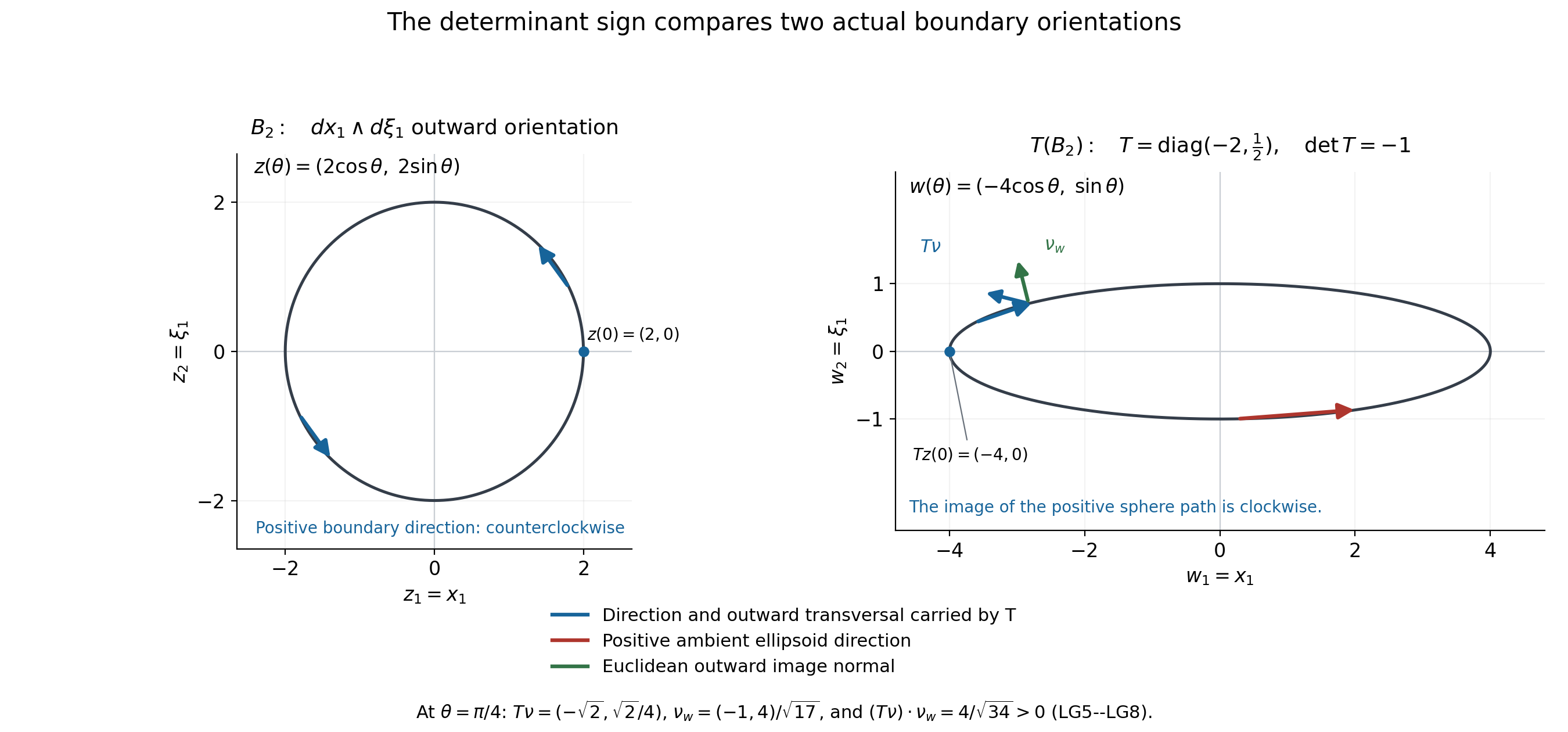
The blue arrows carry the original positive input direction and its outward transversal through the full map in (LO1). The red arrow gives the positive ambient ellipse direction; the green arrow is its Euclidean outward normal. The exact normal dot product and area multiplier are (LO2), and their proof is (LG5)–(LG8). This auxiliary geometric sample depicts no analytic index. Its reproducible figure source, vector image and coordinate record retain every sample coordinate and factor.

14. Complete analytic receivers for the original statements

The full flat matrix-index bridge has its complete finite proof in the matrix-index lesson, (LP3)–(LP14). Its (LP3) starts with the original two ordered errors and a proved trace-norm remainder. Its (LP5)–(LP7) select the full coordinate degree by the actual invertible paths and the finite Laurent identity. Its (LP8)–(LP12) retain every intrinsic derivative and later contraction, cancel repeated derivatives by the explicit coordinate-label involution, and count every remaining ordered exterior word. Therefore the same original finite calculation proves the direct values used in Section5 here, independently of a cited algebraic index theorem. The separate exterior-reduction lesson proves the same calculation independently in (OE1)–(OE17). Its proof retains the full ordered coefficients, coordinate selection, exterior multiplicities and cutoff primitive.

In dimension one the finite choice is $N=2$; in dimension two it is $N=4$. The entire finite coefficient is respectively the $n=1$ and $n=2$ instance of the displayed (LP11), before its exact binomial and factorial cancellation in (LP12). The proved cutoff primitive (BN1)–(BN5) then gives, with the original outward orientation, $$D_1=-(-2\pi i)^{-1}{0!\over1!}={1\over2\pi i},\qquad D_2=-(-2\pi i)^{-2}{1!\over3!}={1\over24\pi^2}. \tag{LC1}$$ Applying those proved formulas to both original symbols $a$ and $a\circ T$, whose full symbol and inverse bounds are (LT1)–(LT7), and then using the complete original boundary comparison (LG1)–(LG11), proves (LS8) and (LS9). For every dimension, the same argument uses the full unchanged coefficient in (LS10), giving $$\begin{aligned} \operatorname{ind}(a\circ T)^w &=D_n\int_{\partial B_R}^{\Omega}T^*\operatorname{Tr}(\theta_a^{2n-1})\\ &=D_n{\det T\over|\det T|} \int_{\partial B_{R'}}^{\Omega}\operatorname{Tr}(\theta_a^{2n-1})\\ &={\det T\over|\det T|}\operatorname{ind}a^w. \end{aligned} \tag{LC2}$$ Here both original bounded Weyl operators have the actual same Hilbert domain and target; each is Fredholm by IP14 and (LT1)–(LT7). Both radii obey the full inequalities in (LG9). The complete beta moment and its nonzero value were retained in (LG11) before division; the determinant sign and the positive surface multiplier were proved in (LG5)–(LG8). Thus this closes (LS10)–(LS11) without replacing any original object or orientation. The complete reflected bounded example (MI1)–(MI2) in the matrix-index lesson, with every denominator derivative proved in its Section10.2, and the literal reciprocal differential (LI2) here give the indices $+1$ and $-1$ in Section7. The two exercise solutions then use only (LC2), (LC1), and the finite graded matrix trace already proved in (EF1)–(EF4).