Global boundary operators, compressed wave fronts, and normal extension
Written and dedicated to the public domain by Codex, September 2026 (CC0).
The local half-space calculus already tells us how a totally characteristic operator acts near one boundary chart. On a manifold, the same calculation must survive changes of coordinates, corners in the operator kernel, and the distinction between an ordinary normal derivative and a vector field tangent to the boundary. This lesson builds that global calculus, proves its wave-front rules, and then uses the exact boundary trace to extend solutions of noncharacteristic equations. A final argument shows when conormal regularity is genuine smoothness up to the boundary.
We keep the original Fourier convention , with inverse factor . A supported distribution is always represented on the closed half-space; a restricted interior distribution is a different object. Matrix products retain their input and output order. All orders of symbols and conormal distributions are real unless a theorem specifies an integer normal order.
The named prerequisites are Singularities along a submanifold and smooth boundary passage, Totally characteristic operators on the half space, From symbol estimates to operators on every Sobolev scale, and Detecting regularity without choosing coordinates. The proofs below reproduce their particular formulas when used, so the global construction remains readable from these exact entry points.
1. Stretched kernels and compressed covectors
1.1. The real projective blowup
Let be a smooth embedded submanifold of codimension in . In coordinates , , . Replace the normal origin by its lines: Here is the actual normal vector, with both signs. Equivalently the model is , , modulo , with . For the chart in which the -th component of the line is nonzero, represent that line by a vector with . Coordinates are , and . On overlaps, These are smooth invertible changes where , including . They give a smooth manifold; the exceptional set is its projectivized normal bundle, and the projection is a diffeomorphism away from . For , there is one line and the local projection is the identity.
To prove independence of coordinates, let be another normal coordinate system vanishing on . Hadamard’s formula gives In a chart , choose an index for which . The new coordinates are , , and the actual transformed tangential coordinate . The denominator stays nonzero locally; all these functions are smooth at . The inverse coordinate change has the same construction. The maps agree away from the exceptional set, and therefore everywhere by continuity, so their cocycle identities hold. This proves coordinate independence and identifies the exceptional transition with the actual normal derivative.
If vanish on , their pullbacks have the form by the same integral formula. Wherever the normal derivative of on the line is nonzero, , and extends smoothly. These ratio charts are thus intrinsic. No positive-ray quotient replaces the projective quotient in this construction.
1.2. The positive corner and its exact coordinates
For boundary charts on two manifolds, keep and their positive normal rays. The projective interior normal cone at the corner is . Its coordinate and the radial coordinate are At , records the ray; the projection collapses this interval to the original corner. The two side faces are , where , and , where .
Boundary coordinate changes have normal parts , , with . Set , . Their exact lifted law is The denominator is strictly positive on the entire closed interval: , , and both coefficients are positive. The tangential coordinates are the original coordinate changes evaluated at . Thus the full lift is smooth up to every face and corner, and its inverse is the lift of the inverse changes. It preserves each side face and multiplies by a smooth positive function. These laws glue the stretched product intrinsically.
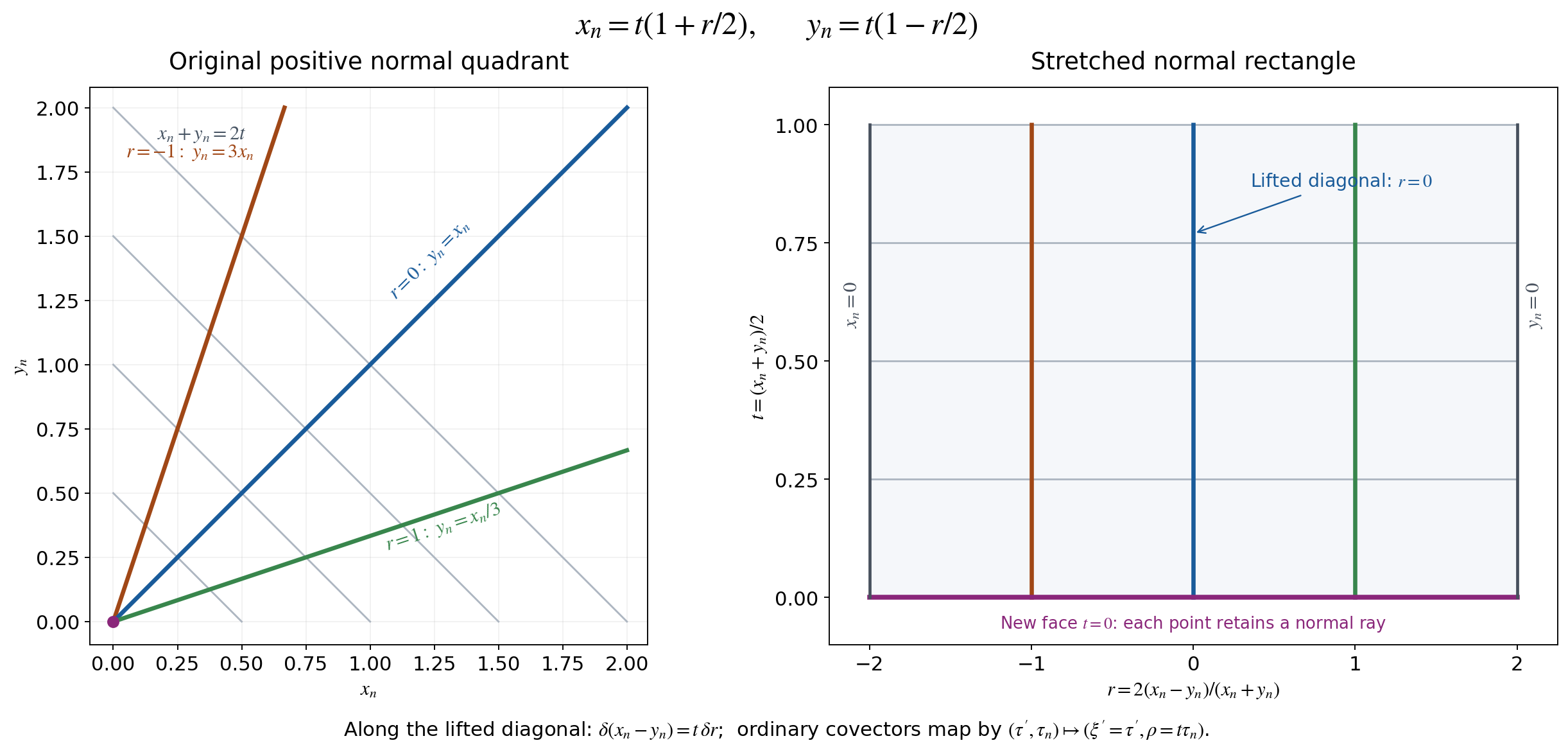
Figure GL-F1. The two panels retain the exact coordinates in (GL4). The new face retains the ray when both normal variables vanish. The lifted diagonal crosses that face. Only the two normal variables are drawn; tangential coordinates and covectors retain their full dimensions in (GL7)–(GL10). Reproducible source: ../figures/global_compressed_corner_geometry.py.
For the square of one manifold the interior diagonal lifts to The projection restricts to , a diffeomorphism with the original diagonal. The lifted diagonal avoids , and is transverse to because its tangent includes the direction. This proves all these assertions at boundary points as well as in the interior.
1.3. The compressed bundle and both natural maps
Pull back by (GL6). In local coordinates its covectors have the form . The normal differential of the projection at the lifted diagonal is This follows by differentiating at . Dualizing gives the natural map from the ordinary cotangent bundle: It is an isomorphism for . At its kernel is precisely the ordinary conormal line to the boundary, and its image is the hyperplane , canonically . The compressed fibre itself still has dimension ; its other covectors have not been discarded.
The dual anchor is Its smooth sections map bijectively onto smooth vector fields tangent to the boundary. Indeed a tangent normal coefficient vanishes at and equals . This constructs its smooth inverse coefficient. Uniqueness follows in the interior and hence at the boundary by continuity.
For an exact coordinate law write , , . In the interior a compressed covector is . Differentiating the original coordinate functions, without dropping terms, gives These expressions extend smoothly to the boundary. There their determinant is ; locally in the collar the matrix is invertible, and its inverse is furnished by the inverse boundary coordinate change. The law agrees with the pulled-back conormal law in the interior by (GL7)–(GL8), and hence agrees everywhere. It proves the intrinsic bundle identification, both anchors, and the invariant hyperplane .
1.4. The original symplectic form and density
In the interior substitute the full formula into the ordinary cotangent form . Since , its exact expression is It is nondegenerate for . The factor is a boundary singularity; there is no smooth symplectic form asserted there. In the indicated order of coordinates, For the sign, move the original ordered pairs to the displayed base-then-fibre order; the number of transpositions is . The density law is intrinsic because (GL11) was pulled from the original cotangent form. Its singular factor remains explicit.
1.5. The full stretched kernel for every symbol order
Let , , in the local half-space calculus. Keep its exact inverse Fourier distribution Oscillatory integrals are defined by the cutoff-independent distribution construction in (C4)–(C5). No residual assumption is made. Differentiation in raises the amplitude order by its exact degree; integration by parts in to a degree exceeding that order plus proves that is smooth off , with arbitrary decay in , uniformly with every base derivative on compact sets. Near its full phase and amplitude exhibit a conormal distribution of order by (C16), with ambient dimension and codimension .
The Fourier support in the original definition implies . In fact the partial Fourier transform of is supported in ; inverse transformation evaluates it at , with the original inverse Fourier factor. At the distribution is already smooth, since that point is away from . Its vanishing on therefore makes every derivative vanish on .
The determinant of (GL4) is , so a kernel half-density pulls back with coefficient . Put . The entire formula is Thus both square-root factors, the normal Jacobian and the complete argument of are retained.
Near the lifted diagonal . In (GL13) change only the integration variable . Its positive Jacobian cancels exactly the displayed , giving The amplitude has all order- estimates on compact base sets: an -derivative gives or ; the latter has the original order . A -derivative has the bounded factor ; frequency derivatives lower the order normally. The same argument handles any iterated mixed derivative. Equations (GL14) and (GL15) are exact descriptions of the same kernel, not a substitution omitting a density factor. They prove that is conormal along , smooth in .
At , the last argument of is , so the preceding support argument gives side flatness, including all and tangential derivatives. At , that argument tends to minus infinity. Its derivatives and the displayed prefactor grow only as fixed powers of . The arbitrary large- decay absorbs each such power, proving flatness there as well. These estimates are uniform for compact ranges. Off , the same Fourier argument proves smoothness.
1.6. The exact principal half-density and inverse reconstruction
In the full amplitude of (GL15), the difference from its value is Retain this entire integral. Integration by parts in , using , changes it to the exact order- amplitude A compact cutoff in on this chart is independent of and does not change that calculation. The defining cutoff limit justifies the integration by parts, by (C4)–(C5). Hence the principal conormal half-density of , in the parametrization , is precisely the class of For , the additional is still present. Comparing (GL18) with (GL12) makes its scalar coefficient a principal symbol on the compressed cotangent bundle. The full remainder is (GL16)–(GL17); it has not been removed from the original kernel. The coordinate invariance follows from the full determinant law (C19)–(C20) and the actual conormal coordinate change (GL10). In the intrinsic convention of (C21), the half-density in (GL18) has symbol order : its fibre half-density has dilation degree . Dividing the original principal half-density of by (GL12) leaves the ordinary scalar or matrix symbol order . Neither convention changes the amplitude or the original operator.
Conversely, take a compactly supported conormal family along , of this order and smooth parameter type, flat at both side faces. For its inverse kernel is These are the inverse of the full coordinate and prefactor formulas, not just their diagonal restrictions. Near , pull back an oscillatory conormal amplitude for by this smooth map. Its normal phase is . The change has positive Jacobian , which cancels the prefactor in (GL19). The resulting amplitude has order with all base derivatives, including , by the same product and chain rules used for (GL15). Compact localization and the full amplitude reduction (C5) therefore give a smooth -dependent inverse Fourier symbol of order , with all finite-seminorm bounds.
Away from , (GL19) is smooth. Flatness at gives arbitrary decay as : each -derivative introduces at most one additional power of , absorbed by another flatness order. Flatness at gives a smooth zero extension at . Compact tangential support controls ; all these far contributions are Schwartz in , uniformly with every -derivative. If is supported in , then is supported in , since . Its base derivatives thus have every original estimate.
Define the exact symbol The near contribution is order by the preceding reduction and the far contribution is residual. Since for , This proves lacunarity with its exact sign and Fourier constant. Thus , and (GL13)–(GL15) recover the original half-density kernel exactly. Fourier inversion proves uniqueness of the symbol on , and smoothness in gives uniqueness at zero. This proves the compact local converse as well as the forward statement for every real .
1.7. The exact boundary action
Let be smooth up to the boundary with compact support. Write , . At fixed , the actual changes of integration variables are Thus the full operator action, interpreted as a distributional pairing at the diagonal, is For a forward symbol, compactly localize the base variables on the output region; (GL14) retains the same uniform side estimates there. For an inverse kernel its given compact support provides this localization. Choose a partition in which is one near its origin and supported away from . On that part the smooth conormal family and the compact smooth test function in (GL23) converge, with every derivative, as decreases to zero. Oscillatory formula (GL15) justifies the convergence: integrate by parts in its normal base variables to an order exceeding the amplitude order plus , exactly as in (C4). The resulting integrable frequency majorant is uniform in .
On the complementary part the kernel is a smooth function. Near , every , or integration-variable derivative of (GL23) introduces only a fixed negative power of . The arbitrary side-flatness order in (GL14) absorbs that power. Near , the same statement follows from smooth flatness at that side. Away from those sides all factors have ordinary compact smooth bounds. Dominated convergence, including each derivative, proves the boundary limit The second equality uses the full change , , and . The last equality is exact partial Fourier inversion at normal frequency zero. The preceding localization and integration by parts justify both equalities even when is not a function at . When , the tangential integrals have dimension zero and the factor is one. This is the full boundary action, with all orders and all kernel factors, and it agrees with the original jet formula (5.2) for .
2. Proper global operators and conormal smoothing
2.1. The global kernel and its actual pushforward
Choose a smooth function on the stretched square, positive off its new face and vanishing simply on that face. Near a boundary diagonal point it can be the original . Define the order- class by kernels represented as Here conormality at the new face has precisely the smooth family meaning specified before (GL1). A bundle kernel additionally has values in . Multiplication by its smooth frame changes is included in the conormal topology.
There is a well-defined pushforward despite the separate factor . Indeed, in the original normal chart, let a test half-density have coefficient . Its pullback has coefficient , since the absolute normal determinant is . Thus the actual pairing is The conormal family is a smooth distribution-valued function of . On a compact interval its pairing with the smooth compact test family is bounded by finitely many test derivatives and symbol seminorms, by (C4). The integral is consequently well defined and continuous. The blowdown has compact projective fibres, so the inverse image of a compact test support is compact; away from the corner it is a diffeomorphism. Those facts reduce the general pairing to finitely many such charts. Equation (GC2) is the complete meaning of pairing with the pulled-back test half-density. Neither square-root factor is separately discarded, and no pairing of an arbitrary distribution with a nonsmooth test coefficient is asserted.
If is another admissible defining function, Hadamard’s formula gives , with smooth near the new face. Away from that face both functions are positive. Hence Multiplication by , and by its smooth inverse, preserves the conormal class and side flatness. The kernel, its pairing and its order are independent of this choice.
Every compactly localized kernel of (GC1) is the original half-space kernel of a lacunary order- symbol by (GL19)–(GL21). Away from the lifted diagonal the localized resolved coefficient is smooth, and the same inverse gives a residual symbol. The latter assertion also applies between distinct boundary charts: coordinates in the two charts may be used as the two independent tangential variables in the smooth kernel; there is no conormal singularity to align. Near an actual diagonal point use the same coordinate chart on both factors. Interior charts give the ordinary conormal pseudodifferential kernel by (C18).
The local theorem on smooth inputs therefore proves a continuous map For fixed input support and a fixed output compact set, only finitely many product charts occur. Each local estimate uses finitely many derivatives of the input, and the sum of these estimates is finite. This proves the stated LF-to-Fréchet continuity. Formula (GL24) supplies its boundary value, and the original formula (5.2) supplies every normal jet. Conversely the local quantizations have exactly (GC1) by (GL13)–(GL18), so this kernel description and the patched local definition determine the same class. We denote it by .
To check coordinate invariance at all orders, the stretched coordinate change is (GL5), its conormal change is (GL10), and its complete amplitude and determinant are (C19). Reducing that entire amplitude by (C5) gives the transformed symbol, with the full order- remainder after terms. All frequency factors created by a base derivative pair with a frequency derivative and retain order . Thus the operator class, not only its leading term, is coordinate invariant. The local construction and the pushforward above agree in the interior and then as distributions by the same conormal family pairing (GC2).
2.2. The symbol quotient and actual realization of every symbol
For a compressed symbol , the original principal half-density of the kernel is the class of The singular half-density multiplying is the invariant absolute symplectic half-density in (GL12). The complete determinant law (C20) therefore gives a scalar symbol, or a section of , on , of ordinary order , modulo order . Both (GL16) and (GL17) remain its actual lower-order kernel remainder. Define using every local compact base set, all base derivatives, and the frequency bound . The fibre transformation (GL10) and its inverse have smooth bounded coefficients on each compact chart; the chain rule proves that this definition is intrinsic. The leading symbol map has kernel exactly , by the local normal-form kernel assertion (C21).
We prove surjectivity while retaining the original prescribed symbol. Choose a locally finite cover by precompact boundary or interior charts , with locally finite closures. Choose a partition with support in these charts and equal to one on a neighborhood of . For a given symbol , compactly localize a full representative in the -th frame so that it equals on that neighborhood. In a boundary chart take exactly the lacunary modification Keep : the bracket is residual by the full Taylor integral (4.8), and every original symbol seminorm remains controlled. Quantize the first term and set in boundary charts, using ordinary quantization for interior charts. The sum is locally finite and has order . Its two support projections are proper: above a compact base set only finitely many chart closures occur, and both factors in each term have compact support in that chart. The leading term is . Multiplication on the input has its complete product remainder, of order , from (8.3); near the working diagonal. The residual bracket in (GC6) has not become an equality between the original full symbol and its modification; it is explicitly the error in this realization. This gives both quotients with the same isomorphism when the operator spaces are restricted to proper support. The bundle version follows in the same charts, with the actual frame transitions and (GC5).
2.3. Proper composition, adjoints and all asymptotic remainders
Let and be properly supported. For every compact output set the support of meets only a compact set of intermediate variables, and that compact set meets only a compact input set under . The reverse argument starts at a compact input set. This proves proper support of the composed operator and permits all intermediate partitions to be finite on the compact sets under consideration.
We give the localization argument, since a residual kernel at the new face need not be a smooth kernel on the original square. Localize near an output-input diagonal point. A sufficiently small common chart contains both variables. Split the intermediate variable into a slightly larger part of that chart and its complement. On the complementary part both kernels are separated from their actual diagonal, so their resolved coefficients are smooth with side flatness. On the chart part use the original local ordered product theorem (8.1)–(8.3). Any localization of either factor off its own diagonal gives a residual symbol by (GL19)–(GL21). That theorem then gives a residual product: its finite-order bound holds for every real order assigned to the residual factor, while its complete far term (8.2) is residual as well.
For clarity, this also handles two different boundary charts. For a localized rectangular smooth kernel , with output and input coordinates taken from their respective charts, the literal inverse is This is the same (GL19) inverse written at fixed , with all chart half-density factors included in . Resolved smoothness, side flatness, compact chart cutoffs and the full far estimates of (GL19)–(GL21) make residual and lacunary. The two coordinate tuples both range in Euclidean half spaces, so the original local product theorem applies to these rectangular symbols with the intermediate coordinate tuple used as its common integration variable. If only one factor has a diagonal singularity, use its chart for the intermediate variable and its adjacent variable; the other is represented by (GC9a). If neither factor has a singularity, either choice works. Near a fixed output-input point off the diagonal, use disjoint neighborhoods of those two points and split the intermediate variable into their neighborhoods and the complement. At least one factor in each term is then separated from its diagonal, and the preceding argument proves a residual result. This proves the required smoothness off the lifted diagonal, its family regularity at the new face, and its side flatness; it does not replace a corner residual by an ordinary smoothing kernel.
In the common chart the complete product symbol is , where and are the actual (8.1) and (8.2), with the original factor order before . The full expansion is The exact far contribution is part of . All its seminorms and the remainder seminorms are controlled by finitely many seminorms of the two original factors, by that local proof. Hence For matrices this is ; no order is exchanged. The same argument proves that the residual class is a two-sided ideal among properly supported operators of any finite order.
Transposition of the stretched square exchanges and sends to , keeping . Its kernel half-density law is Conormality and side flatness are preserved. The local adjoint (7.3), including the residual adjoint of , gives . Thus Proper support is preserved by this exchange. All adjoints here use the fixed metrics and the original half-density pairing.
The calculus admits full asymptotic sums. Here is the construction needed later for parametrices. In each chart let be the actual localized symbols to be summed. Choose zero on the unit frequency ball and one outside twice that ball. Choose increasing so that has each of the first seminorms in at most , on the first compact base sets. This is possible because the support has , giving the extra factor ; frequency derivatives of the cutoff have the same bound after the product rule. The exact sum converges in the stated seminorms. For the remainder, its infinite tail lies in ; each of its finitely many low-frequency differences is residual. Lacunarize the full sum by (GC6), retaining the new residual difference, and patch as in (GC7). Each finite off-diagonal discrepancy is residual by the localization argument above. Consequently the global operator differs from every prescribed finite operator sum by exactly the asserted lower-order class. This proves asymptotic completeness, including on the proper-support subspace, without omitting any finite term or its remainder.
2.4. The supported and restricted Sobolev maps
For and every real , the actual local theorem (PS1)–(PS17) gives the supported bound with loss . Smooth coordinate changes and frame multiplications on compact sets are bounded on every real Sobolev scale: integer bounds follow by the chain and product rules, negative integers by their exact adjoints with the Jacobian, and intermediate orders by the Fourier interpolation already proved in the local prerequisite. On a fixed compact input set, proper support and a partition reduce to finitely many of those bounds. A rectangular residual term has every order, so use its original order-zero bound and the continuous inclusion , valid for . Thus, for each compact , there is a compact and a constant depending on finitely many localized full-symbol seminorms such that The supported action is the original transpose action (9.1), so it includes distributions supported at the boundary. Both localizations and coordinates keep those terms; they are not zeroed by a chosen extension. For a nonproper operator the same proof gives local output bounds for compact input.
The corresponding restricted map follows from the exact local quotient map (PS16)–(PS17). Local supported representatives give the bounded map; the local action preserves the full ideal of distributions supported only on the boundary by (9.2), so different representatives have the same interior output. Taking the infimum over representatives in each fixed chart gives the restricted norm bound. Patch the actual quotient maps using the same finite cutoffs. This proves , and the compact-output assertion under proper support. No gain of is asserted when ; the original residual examples prohibit such a claim.
2.5. The supported conormal class and the residual receiving map
For real , let consist of distributions supported in the closed manifold which, in every boundary chart and its extension, are conormal of order to . Explicitly put and require The topology uses all these local seminorms. Multiplication, coordinate changes and finite frame transitions are continuous on those Besov spaces by (C2)–(C3), and (GL9) identifies the intrinsic tangent fields. Moving a coefficient through a word in tangent fields leaves only shorter words with smooth coefficients. Hence (GA1) is intrinsic and agrees exactly with (C15), with the original shift .
The coordinate seminorms can use and . The precise comparison with the original weighted derivatives is where the first polynomial identity defines an invertible triangular change of basis and the second is its inverse. The first follows by and induction: multiplying by on the right gives . These identities retain every lower term and its factor . Tangential derivatives commute with . On compact sets all smooth-coefficient tangent words reduce to these generators. In particular (GA1) makes smooth in the interior by repeated ordinary derivatives there and the local Sobolev estimate.
If is proper, its local conormal preservation theorem 11.2, with the actual index , gives continuously, for every real . Finite localized product estimates prove the global continuity as in (GC14). An off-diagonal resolved term is residual and obeys the same theorem in the rectangular chart. The order does not change the conormal index: the local proof factorizes each full tangent derivative of the original operator through an even-order totally characteristic differential operator and applies the order-zero Besov bound to its two complete factors. In particular neither the original frequency nor a positive-order remainder is omitted.
There is a stronger receiving statement for a residual operator . Fix an input compact set and . For every tangent word , the composition is still residual, by the local product formulas and (GC10). Its order-zero bound therefore gives The inclusion is immediate from the dyadic and norms. Any compactly supported distribution of order belongs to for : its Fourier transform is bounded by , and the weighted square integral converges for exactly that strict inequality. The same estimate is uniform on a family with fixed support and bounded distribution-order seminorm. Thus with the explicit fixed-Sobolev-source continuity in (GA4). This is a conormal receiving map, not an assertion that a residual operator produces a smooth function at the boundary.
2.6. Approximation which preserves the original closed support
Let have integral one and support in the open positive half-space. Set and . For a distribution supported in , this convolution is smooth and supported in , where . Its support remains in one fixed compact enlargement when the input support is fixed and .
We prove convergence in the conormal topology, including its weighted normal derivatives. Write , . Integration by parts in the distribution pairing gives the exact identity Indeed has coefficient , whereas has coefficient . Their difference is . Both terms and their sign are retained.
Define , , and let denote convolution by . Every is smooth, has the same compact positive normal support, and for . Repeating (GS1) proves Tangential derivatives commute with all these convolutions. These are equalities on distributions; no boundary derivative term is dropped.
The Fourier multipliers satisfy, for each fixed , For small arguments use the mean, the first-moment integral and ; for all arguments use their finite norms. These multipliers commute with the dyadic projections of (C2). Let , , and . The multiplier bound on the -th block is at most . Since each difference multiplier in (GS3) maps to with norm at most . To verify (GS4), split at . Below it the expression is , at most if , and at most otherwise. Above it the expression is .
For , , the actual indices are , , so . Subtract from (GS2). Its term is , and all its terms have the mean-zero bounds in (GS3). Every input has the same Besov index , by the full definition (GA1). Consequently Equations (GA2) and the full product rule now give every original weighted derivative seminorm and every smooth-coefficient tangent word. Thus in , not merely as an ordinary weak distribution, with finite-seminorm control.
Finally choose the locally finite chart partition and input cutoffs near their supports as in (GC7). In each boundary chart use the positive convolution just proved; in interior charts use a compact mollifier whose small translations remain interior. Use the actual half-density and bundle coordinate maps on both sides. Define Choose each chart’s convolution radius no larger than its fixed distance from the cutoff support to the chart edge; a constant multiple of in that chart suffices. On a fixed input compact set only finitely many occur, giving a single compact output set , independent of sufficiently small . Smooth multiplications and chart maps are continuous in (GA1). Since , (GS5) and the full Leibniz rule prove For compact input its output is compact and supported in the interior, including in boundary charts. The convergence is uniform on bounded sets of each fixed compact source, by the displayed finite-seminorm estimates. This proves the required support-preserving smoothing lemma with its original order indices.
3. Dual distributions and boundary traces
3.1. The lowest test order and the dual class
Put . In a boundary chart, let be smooth up to , compactly supported for , and let be its zero extension. Integrating its normal Fourier transform by parts times gives, for , Each displayed boundary jet, including its sign, follows from the lower endpoint in integration by parts. The remainder and all its tangential derivatives are bounded by the corresponding compact smooth seminorms. For any requested number of frequency derivatives, first multiply by powers of under the integral and repeat the same integration by parts with enough extra terms; this gives the full order- symbol estimates. Multiplying by a cutoff equal to one for and absorbing the compact-frequency part into a smooth amplitude yields the exact reduced conormal form (C16). For codimension one its amplitude order is ; order means exactly . If , the first term in (GD1) is nonzero, so a uniform claim of a lower conormal order is false. Hence where a smooth boundary function is represented by its zero extension. The continuous inclusion for is immediate from the symbol orders or the dyadic Besov weights. Interior-supported smooth functions belong to every order.
Define as the ambient supported distributions whose action on every compactly supported smooth boundary function is continuous with respect to the topology, for every . Precisely, for each compact and each such , finitely many defining seminorms and a constant give The action is independent of an ambient smooth extension of : two extensions agreeing on the closed half-space differ by a smooth function vanishing on its interior and to every order at its boundary; the supported distribution annihilates that difference. This is checked in each chart and patched by a partition. The topology on used here is the weak topology generated by all for compactly supported , where .
We prove that the pairing in (GD3) extends uniquely to every compactly supported , . Choose . The support-preserving is smooth with support in a fixed compact , and (GS7) gives convergence in . The bound (GD3) at order makes converge. If another smooth sequence converges to in the same order, its difference has pairing tending to zero by that bound, so the extension is unique. To show continuity on , use (GD3) at on the approximants and take the limit. The inclusion is continuous, which supplies the finite bound. No convergence in the same endpoint order has been assumed. This constructs the full pairing and the stated weak topology.
3.2. Interior restriction, absence of boundary-supported elements, density
If vanishes on all tests in the interior, then for each compactly supported choose . Each is smooth and supported in the interior, so . The convergence in and the extended continuity prove . Smooth boundary tests are among these , hence as an ambient distribution. Therefore In particular no nonzero distribution supported only on belongs to . This follows from the exact density argument, not from a mistaken identification of the two distribution spaces.
Smooth boundary functions are weakly dense in . First every smooth boundary function defines an element of : on a compact test support, multiply that function by a smooth compact cutoff and pair it with the supported conormal distribution. In the normal form (C16), the compact smooth factor has rapidly decreasing normal Fourier transform. Integrating the full symbol amplitude against that transform bounds the pairing by finitely many seminorms for every real ; the normal-form topology comparison in (C16) gives the corresponding bound. Interior terms use the ordinary distribution pairing. Thus the smooth approximants below really belong to . For a compactly supported , define . The adjoint of each local term in (GS6) is convolution with a compact smooth reflected kernel, followed by smooth cutoffs and coordinate/half-density maps. For a distribution , this adjoint is a smooth function of the remaining variable, including at its boundary; on every compact set only finitely many chart terms occur. Thus is represented by a smooth function on . For each fixed of order , choose . By (GS7), in , and the extended continuity gives This is weak density with the actual test topology, for every compact conormal test. Together with (GD4), it identifies with its image of interior distributions; it does not make all interior distributions members of .
3.3. The invariant boundary delta and trace
Let be a compactly supported smooth test density on , with the dual bundle coefficient when appropriate. In a boundary chart define the supported distribution density For a new defining function , , the exact distribution density law is : the delta coefficient contributes and the normal density contributes . The tangential density and bundle transitions are the usual ones. Hence is intrinsic, not a choice of boundary coordinate or a half-density shortcut.
The original Fourier amplitude in (GD6) is constant in , with the exact coefficient . Formula (C16) for codimension one therefore gives , that is, The direct Besov estimate uses the same dyadic amplitude bound, so the target topology is included. Define the boundary restriction by The exact conormal order in (GD7) lies above , so the extended pairing is available. Its continuity in follows from (GD3) and (GD7), and its weak continuity in is one of the defining seminorms of . Thus (GD8) is a distribution on the boundary.
For a smooth function up to the boundary, use the positive normal convolution on . It is a unit-mass smooth approximate delta supported at positive normal distance . Consequently tends to , with the full chart density factor. The extension of the pairing in Section 3.1 gives the same limit for . Hence (GD8) agrees with ordinary smooth restriction. Its uniqueness among weakly continuous trace maps follows from (GD5).
3.4. Corrected differentiation with its exact sign
Let , represented as an ambient distribution supported in the closed half-space. Write from (GD8). Define This is the original ambient derivative plus its full boundary delta correction, with no suppression of either term. The sign follows first for a smooth from Both identities are direct distributional product rules, since . Adding the term in (GD9) makes the supported representative of the ordinary interior derivative for smooth .
We prove membership in for general . Let be a compact smooth boundary test, and distinguish its ambient smooth extension from its supported zero extension . In the pairing, is the pairing with the zero extension of . The full distribution identity is Therefore the two terms in (GD9) combine exactly to The ordinary differential map is continuous: the normal derivative multiplies the full conormal amplitude by and differentiates its smooth base coefficient, while tangential derivatives differentiate that coefficient; (C4)–(C5) control all remainders. Equivalently it is the exact order-one conormal map (C17) with compact support. If , then , so (GD12) and the defining estimate at order show that . The map is weakly continuous: for each compact conormal test , its defining functional is , another test in . In the interior the delta term vanishes, so .
The uncorrected derivative can fail to lie in . For example choose a smooth with nonzero boundary value. By (GD10) the ambient derivative contains the nonzero boundary-supported term , while is in . If were in , subtracting would put a nonzero boundary-supported distribution in , contradicting (GD4). This proves the distinction, rather than treating the two derivatives as identical presentations.
3.5. Proper totally characteristic operators on the dual class
Let be properly supported. Its formal adjoint preserves continuously for every , by (GC12) and (GA3). Given a compact output test , proper support places in a compact set depending only on the support of ; its full conormal seminorms are bounded by finitely many input seminorms. To use these bounds with complex-linear distribution evaluation, take a compact dual-density test and put , where the exact metric-and-density map is defined in Section 3.6. The bilinear transpose is . The actual linear dual action is The two conjugate-linear maps in this transpose make it complex-linear. Section 3.6 proves the identity with the full bundle and density factors and proves that its conormal-test seminorms have the required finite bounds. For a smooth boundary test, (GD3) therefore proves . For smooth , the local adjoint identity (7.6), transported by those exact maps, gives the original kernel action. For general , (GD5) and weak continuity extend that equality; in the interior it matches the usual distributional operator. The coefficient order and bundle maps remain those of the original , with no scalar commutation of matrices.
The boundary jet formula extends as well. In a local half-space chart, let , and define the -th interior normal derivative of by iterating (GD9), then taking (GD8). For smooth , the exact formula is Every coefficient in the inner sum and the outer binomial factor is retained. Its -th summand has order . The tangent boundary operator acts continuously on boundary distributions after compact localization; this is the ordinary local symbol action. The left and right sides of (GD14) are weakly continuous in by (GD8), (GD9), (GD13) and the boundary operator continuity. Smooth functions are weakly dense by (GD5), so (GD14) holds for every . It is a statement about their actual boundary traces, not about an arbitrary supported representative’s raw distributional normal derivatives.
3.6. Linear distribution tests and Hermitian adjoints
The distributions in (GD3), (GD11), (GE9), and (GT6) evaluate their dual-density tests complex-linearly. A Hermitian pairing, with inner product linear in its first argument, is conjugate-linear in its test. We construct the exact map between these evaluations. This also fixes which operator must be transposed in (GD13).
Let be the density bundle, let be a smooth positive density, and choose smooth positive Hermitian metrics . The test for an -valued distribution is a compact section of . Define This is conjugate-linear in , and it is bijective in each fibre: in a local frame its matrix is invertible because the Hermitian metric is positive and is nowhere zero. Its inverse is smooth and conjugate-linear. Both maps retain the density and the full metric matrix. Define the antilinear-test evaluation of the same distribution by Thus is complex-linear in the distribution and bijective. Supports agree, since and its inverse preserve the support of every test. Evaluating fixed tests on either side proves continuity in both weak dual topologies. This is the pairing used in the linked local Theorem 9.1(a),(b).
Here are the density factors when the original kernel acts on half-densities. For , write its function-section presentation and its Hermitian adjoint as Indeed carries exactly to the intrinsic half-density pairing. Applying the defining adjoint identity for , then this map and its inverse, proves the second equality. The factors and stay in the operator product. For an operator already acting on function sections, means its adjoint for the displayed .
For compact smooth , set . Then The dot here is evaluation of a dual-density section on its vector, with no complex conjugation. Two conjugate-linear maps surrounding the linear give a complex-linear . The integral identity characterizes this transpose on smooth tests. Proper support supplies its compact test domain, so it also defines the distributional action in (GD13). Applying (DT2) and (DT4) gives Every equality has its stated test space. The same original operator therefore acts in both evaluations.
For completeness these maps preserve every original conormal-test order. Locally write , where includes the full positive density coefficient and the metric matrix. For , the complete derivative formula is Complex conjugation reflects the full Fourier variable , preserving the original radial dyadic Besov weights. Smooth compact multiplication obeys the finite seminorm bounds of (GA3). The product rule for every boundary-tangent word gives the same finite sum, with all derivatives of ; the smooth inverse matrix has the same property. Hence , and their versions preserve every filtered continuously. Combining this fact with the adjoint estimate preceding (GD13) proves the required transpose estimate, with its actual input and output compacts. (GD3) proves that , and evaluation of each fixed transposed test proves weak continuity. The maps (DT2) are also bijections of the corresponding conormal dual classes.
The linear action is independent of the auxiliary metric and density. For two choices let and ; these are smooth linear invertible test maps. Applying (DT4) twice gives exactly For a fixed function-section operator , these equalities follow by multiplying by the stated inverse maps in their displayed order. If one changes a half-density presentation, (DT3) supplies its full additional transport. No density or bundle is silently identified with another.
Two scalar computations test the signs. On the positive half-line take , real , , , and . Then The last two values differ. In (DT5) the test evaluation is antilinear, and its factor gives , exactly the original action. In a flat scalar chart let be complex conjugation. Since , one has and . The corrected normal action (GD9)–(GD12) therefore reads The in the second line uses the antilinearity of ; the normal delta in the third line retains its factor . For a variable metric or density the exact test map is , obtained from (DT2). Its full product derivatives of the density and metric remain; the flat formula is asserted only in the stated flat chart.
Finally the normal primitive in Section 5.2 is . Fubini on the compact support of gives its full bilinear transpose and flat Hermitian adjoint: To see the first line, interchange the integrals in ; the coefficient of is exactly the first displayed expression. Replacing by its conjugate and conjugating that coefficient proves the second line. For the real cutoffs chosen in Section 5.2, and supported below , this is exactly its stated . All derivatives of both cutoffs appear in the integer Sobolev bounds. The Hermitian adjoint supplies the negative-order Sobolev estimate there. The bilinear transpose supplies the raw linear evaluations in (GE9) and (GT6), including every coefficient derivative. The boundary jet formula (GD14), weighted extension (GE23), and trace comparison (SC4) therefore use one consistent original distributional action.
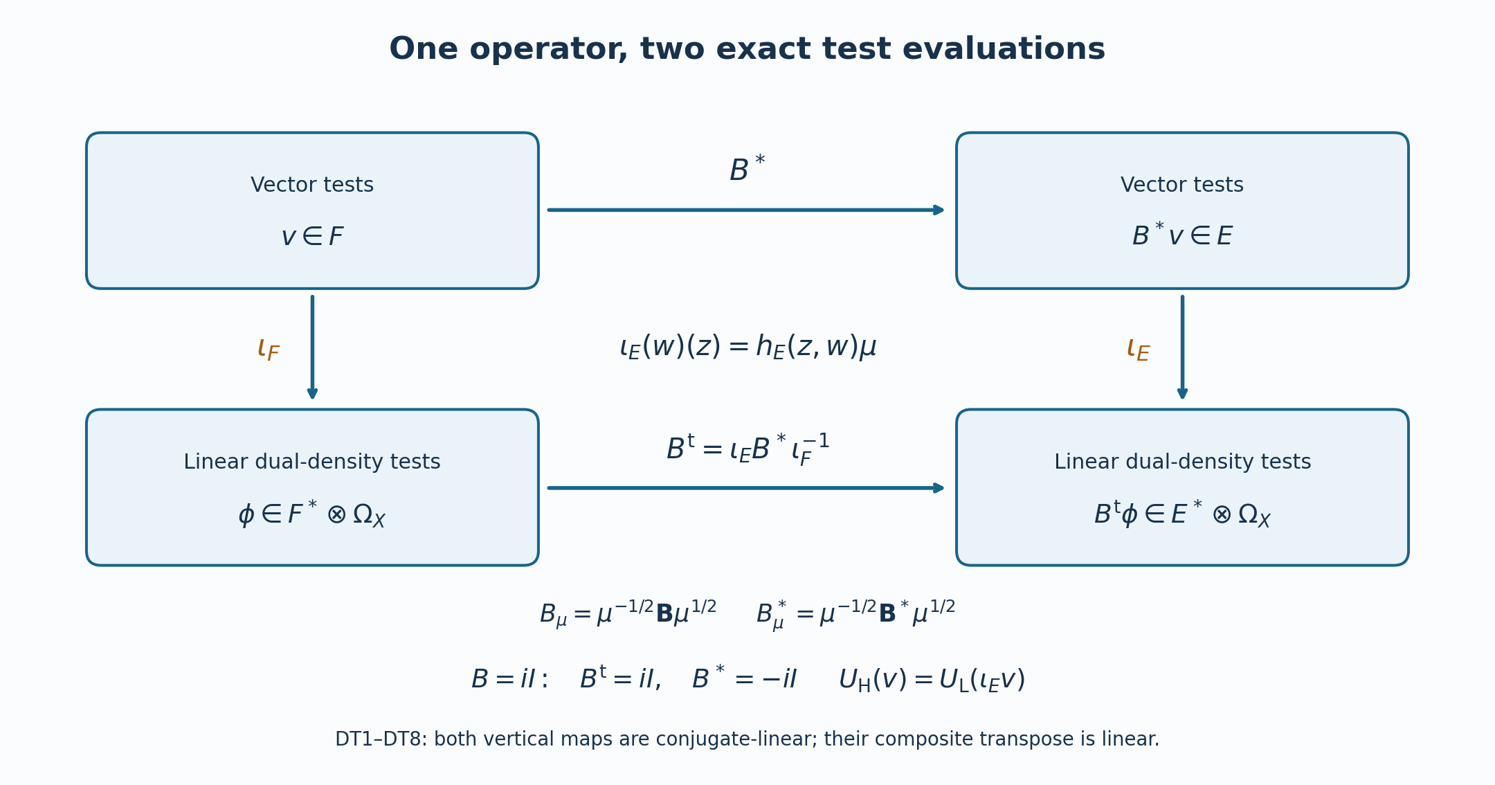
The two arrows include the complete metric and density. Their square commutes by (DT4), and (DT5) transports the same operator to its two dual evaluations. The half-density factors are (DT3), and the scalar phase test is (DT8).
4. Compressed wave fronts
4.1. Ellipticity and the characteristic set at every symbol order
Let and let be its complete local symbol. At a nonzero compressed covector , call elliptic if the two bundle ranks agree and there are a base neighborhood , an open cone containing , constants , and local frames such that The set of covectors where this fails is . Changing the representative by does not change (GW1): is , so for large its ordered Neumann series is invertible. Smooth frame changes conjugate or left/right multiply by uniformly invertible matrices on a smaller compact chart. Thus the definition is intrinsic. The complement of the characteristic set is open and conic; the set itself is closed and conic in .
The inverse in (GW1) has the exact order on a smaller cone. Differentiate : Repeated product differentiation keeps the original matrix order. Every frequency derivative lowers the order by one; every base derivative leaves it unchanged. Multiplying by a conic cutoff gives a global chart symbol of order . This proves the symbol estimate needed for an actual microlocal parametrix.
Here is the complete construction. Choose nested cones and base neighborhoods , with a smooth large-frequency cutoff supported in and equal to one on for large. Set , with the original map . The lacunary realization (GC6)–(GC7) changes this by a residual symbol only. The ordered product gives Suppose the sum has error , residual away from that cone. Its next correction is The actual product is one order lower by (GC9), so the new error is in , still residual off the elliptic cone. The cutoff is supported inside the cone where exists. At each stage the part not cancelled by was already residual; include it in the final residual instead of dividing it by . Asymptotic summation (GC13) produces a single properly supported with the global localized identity and is elliptic on . The low-frequency part and all coordinate-patching errors are residual, and every finite error is retained until its correction in (GW4). The same construction on yields a right parametrix when needed; it is a separate ordered calculation, not inferred by commuting the matrices in (GW4).
4.2. The compressed wave-front set
For a supported distribution , define The zero operator is always an admissible test, with characteristic set equal to the whole nonzero compressed bundle. The identity is an admissible test exactly when . Thus the family of tests is never empty. Every characteristic set is closed and conic by (GW1), and so is its intersection. At a covector outside there is one properly supported order-zero , elliptic there, with . The target cannot be changed to for arbitrary supported distributions: (GA5) receives a residual operator into , and its original corner kernel may fail to smooth at the boundary.
For later use we prove the finite-cover consequence of (GW6). If is empty above a compact , the compressed unit cosphere above has a finite cover by cones where order-zero operators are elliptic and . Choose a smooth partition of unity in those cones at , summing to a spatial cutoff near . Apply (GW3)–(GW4) separately to the symbols , preserving their factor order. Asymptotic summation gives properly supported and a residual such that The missing compact-frequency part is a residual kernel and is included in . Choose the output supports of all in one compact neighborhood of . Then has compact output support; proper support gives one compact input set. Choose a compact smooth equal to one on that input set. The exact identity lets (GA5) apply to the compact distribution , even when the original is not compact. Acting on , every belongs to by (GA3), and by (GA5). Thus . On a noncompact manifold the order obtained from this finite cover may depend on the compact set. Retain the original class , and define its exact local enlargement by
Multiplication and restriction give the injective map . The preceding finite-cover argument proves the exact replacement for the global-order assertion:
For the converse, at any compressed covector over , choose a compact smooth equal to one near . The multiplication operator is properly supported, elliptic at that covector, and maps into the original , by (GW8a). These testers exclude every covector. For the forward implication, apply (GW7) on a compact neighborhood of , then multiply its conormal output by . The maximum of the finitely many conormal orders is one valid order for that compact output. If has compact support, choose on its support; then and (GW8) does imply . In particular the original global-order equivalence holds on compact . No single order is asserted after an infinite exhaustion.
The distinction is necessary. On , of dimension two, choose nonzero and form the actual locally finite supported distribution
Each compact set meets only finitely many summands. The -th summand has normal amplitude with inverse factor , so its conormal order is exactly , by the original codimension-one shift with . It belongs to , including all tangent derivatives. It does not belong to when . To verify the last statement directly, select a bounded interval in tangential frequency on which the squared Fourier transform of has positive integral. On the full sharp dyadic annulus, restrict the normal frequency to strictly inside that annulus. Its squared Fourier integral is bounded below by . The (GA1) Besov factor is , so the resulting norm is at least , which diverges for . Multiplying (GW8b) by a compact cutoff equal to one around its -th boundary support isolates that summand. Thus (GW8b) lies in and has empty compressed wave front, but lies in no . This proves strictness of the displayed injection. The quotient records precisely this failure of one globally bounded order, with kernel of the quotient map equal to the original .
The stronger smoothness conclusion for needs the separate local intersection theorem proved below. It is not being inferred from conormality alone.
4.3. Residual localization and elliptic inclusion
Let have a full symbol of order in a conic neighborhood of a closed conic set . At each choose an order-zero cutoff elliptic at whose large-frequency symbol is supported in a smaller cone inside that neighborhood. The full ordered product expansion (GC9) has every term residual there: derivatives of the cutoff stay in the smaller cone, derivatives of the full symbol of have arbitrary negative order there, and the exact far product term is residual. The coordinate-invariant remainders (GC13) therefore give , after harmless compact spatial localization. By (GA5), . Hence This proves precisely the conormal residual target; it makes no unsupported boundary smoothness claim.
For the elliptic inclusion, let be outside both and , where is proper. Select an order-zero tester elliptic at with . The product has invertible principal symbol near in the original order; its inverse is . Apply (GW3)–(GW5) to , choosing supported in the common elliptic cone and equal to one near . There is an order-zero tester elliptic at and a residual with the exact identity . The first term is conormal by (GA3), and the residual term by (GA5). Thus , giving Every inverse and product has retained the bundle map order.
For a properly supported , the forward inclusion follows by the complementary microlocal division. If , take an order-zero elliptic there with . Construct its right local parametrix as above, so , where is residual and has full symbol equal to the identity on a smaller cone about at high frequency. Choose of order zero, elliptic at , with full symbol supported inside that smaller cone. Put . Since is supported where the full symbol of is the identity, the exact product (GC9) and its far residual give . The product is residual by (GC10). Therefore with . Thus , so The same inclusion holds for an arbitrary ordinary smooth differential operator, including the unweighted normal derivative. We prove this separately because itself is not a totally characteristic operator. For , choose elliptic at with . The left localized parametrix gives , where the full symbol of is exactly one on a high-frequency cone about and is residual. Thus Choose an order-zero tester , elliptic at , with full symbol supported in a smaller cone where microlocally. Then is residual by (GC9), including its exact far term. The ambient supported distribution is again supported in the closed half-space. The local commutators are exactly These are the unmodified (5.1), with and all signs retained. They first hold on interior compact smooth functions. Theorem 9.1(e) in the local prerequisite approximates every supported distribution weakly by such functions; each term in (GW12b) is a composition of weakly continuous operators on supported distributions. Taking that limit proves the same identity for the actual supported representatives, including any boundary deltas.
Write . Since the full symbol of is constant one on the working cone, the symbols and vanish there to every symbol order. Apply on the left in (GW12b) and use (GC9): each resulting product is residual. The exact identity is therefore a sum of residual operators applied to supported distributions, or . It belongs to by (GA5). On the other hand by (GW12a), and the ordinary differential map (C17) gives ; applying preserves that class by (GA3). Hence , so Smooth coefficient multiplication is in , and (GW12) applies to it. Finite sums and products of the with such coefficients therefore give the same inclusion for every ordinary smooth differential operator. The proof has kept the normal term in (GW12b); omitting it would make the boundary claim unjustified.
4.4. Interior comparison and a noncharacteristic boundary
In the interior, (GL8) is the ordinary cotangent identification. Localized global -operators are ordinary pseudodifferential operators there by (GL13)–(GL15), and every ordinary properly supported local operator can be realized with the same interior kernel in the global class, using (GC7). Also restricts to in the interior by (GA1): every derivative is a combination of tangent derivatives on a compact interior chart, and the local Sobolev estimates give all smooth derivatives. Both implications in the tester definition therefore give the exact equality
Let be a smooth ordinary differential operator of positive integer order , and let vanish simply at the boundary, with , , in a chart. No original coefficient is removed. The complete differential expression retains every lower-order and tangential term; the displayed factor order is valid because commutes with . Thus . At , all principal terms except contain a positive power of . Its complete boundary principal compressed symbol is If the boundary is noncharacteristic, the original leading normal coefficient is invertible. Equation (GW15) is invertible exactly when ; its boundary characteristic set is precisely the embedded tangential hyperplane , with the zero section excluded. Applying the full inclusion (GW10) to the actual operator yields For , is multiplication by its original invertible coefficient under the corresponding noncharacteristic hypothesis; the same parametrix gives (GW16) with an empty boundary characteristic set. Formula (GW14) is not used with a negative power.
5. Noncharacteristic normal extension
5.1. The exact local conormal seminorms
Fix compactly contained in the coordinate chart, and use a slightly larger compact . For , the conormal topology on supported tests is generated by Smooth chart cutoffs are inserted in each norm. Formula (GA2) proves that these weighted normal derivatives span exactly the same filtered family as all words in and . No lower term of the triangular polynomial relation is dropped. Tangential differential operators , of any fixed finite order, and their formal transposes map each continuously into . To verify this, expand a tangent word through : every resulting term is another finite tangent word with smooth coefficients, including the derivatives of those coefficients. Multiplication by a compact smooth coefficient is bounded on each by (C2)–(C3). The number of seminorms needed depends on the actual tangential order; no relation to the normal order is assumed.
For later use, the dyadic Fourier estimates give, for every real , On the low-frequency block the first norm controls the left side. On the -th high block, ; multiply its norm by , use Plancherel for each , and take the supremum over . This proves (GE2) without a boundary norm convention or an omitted tangential term.
5.2. The normal primitive gains one conormal order
For with support in , put Choose a fixed normal cutoff equal to one on and supported in . Then has compact support in the interior for each such , although the distance of that support from the boundary need not be uniform.
We first prove that the localized Volterra operator is bounded on for every real , with fixed chart cutoffs. For this ambient-space estimate, choose a smooth input cutoff equal to one on the original , extending a short distance across , and write the integral as . For the original interior-supported this is exactly (GE3) after multiplication by . The smooth cutoff is necessary in the negative-order dual estimate; a sharp input cutoff at zero would create an unjustified boundary multiplier. For , Cauchy–Schwarz on the finite normal interval gives . For a nonnegative integer , differentiate at most times. Tangential derivatives commute with the integral; each positive normal derivative of is the corresponding derivative of of one lower order; derivatives of multiply the same expressions. Thus is bounded. Choose these fixed cutoffs real valued. The Hermitian adjoint has the reversed integral . The bilinear transpose has the full factor ; both identities and their exact relation are proved in (DT10), Section 3.6. Its derivatives obey the same integer estimates, including the derivatives of the smooth , so duality gives . For a real , choose integers . The dyadic operator matrix estimate between the two Sobolev endpoints is the one proved from (C2)–(C3): after weighting by , it decays geometrically in . Summation proves the claimed bound, including negative indices. The constants depend on the fixed cutoffs, not on how near the input support is to .
Now set . We prove the stronger precise primitive estimate since . For a tangent word with no normal derivative, , so the Volterra bound controls its norm by the corresponding seminorm. Apply (GE2) to gain the missing one degree. Its tangential derivatives are , and its normal derivative is . The same Volterra estimate controls all these norms by a finite set of (GE1) seminorms for .
For a word with positive normal order , preserve its entire normal weight: The right side has a factor times a tangent word in , so its norm is controlled. Its normal derivative is This is the full product rule, including its term; when that term is absent and the earlier calculation applies. The tangential derivative is , again a smooth multiple of a tangent word. A cutoff derivative contributes , which has the same bound. Applying (GE2) proves the estimate for each word, and summing finitely many words proves (GE4).
5.3. First-order normal equations at every test order
Let be a finite matrix of tangential differential operators with smooth coefficients of arbitrary finite orders, and let the extendible interior vector distribution solve We prove that has a unique extension in . For interior compact smooth tests supported in , we first establish the bound for every real , with a finite depending on . Since is extendible, choose one ambient distribution extension temporarily. On a fixed compact set it has finite order , so its action on interior is bounded by finitely many seminorms. Choose . Fourier inversion and Cauchy–Schwarz bound those seminorms by , and a slightly larger norm bounds by a geometric dyadic sum. Choose sufficiently negative that . The term of (GE1) then proves (GE8) for . The extension’s boundary values do not enter this interior-test estimate.
Assume (GE8) at some . Let be (GE3), the fixed cutoff, and use the bilinear distribution pairing. The formal tangential transpose retains every coefficient derivative and reverses the matrix maps. Since on the support of , the exact equation (GE7) gives All arguments of in this formula are smooth and supported in the interior. The functional is continuous on compact tests for every : for this is its defining property, and for the inclusion is continuous. The operator and the normal cutoff multiply continuously by Section 5.1, regardless of the tangential order of . Apply the induction hypothesis and then the full primitive estimate (GE4). It yields (GE8) at , with finite constants and a possibly larger finite . By induction (GE8) holds at for every integer . For an arbitrary real , choose with ; the continuous inclusion gives the desired bound.
Construct the supported extension rather than silently identifying it with the temporary ambient one. For a smooth boundary test supported in , let be (GS6); it is smooth, supported in a fixed compact subset of the interior, and converges to in for every , by (GD2) and (GS7). The bounds (GE8) make exist: use the bound at such a on differences of approximants. The limit is independent of the particular one-sided smoothing family because both approximations converge in the same topology. The uniform (GS2) multiplier estimate and (GE8), followed by the continuous inclusion from to a larger test order, prove for every a finite estimate of the form (GD3) for . The smooth-test topology bounds those conormal seminorms by finitely many ordinary smooth seminorms, by (GD1); thus is a distribution on the closed chart. The supported-distribution duality of local Theorem 9.1(a),(c) gives its ambient supported representative. Its interior restriction is , since is an approximate identity there. By (GD4), no second extension of exists. This proves the first-order existence and uniqueness in the exact dual topology.
5.4. Full normal order by the actual companion system
Let and retain the original normal-monic equation Each is an arbitrary finite-order tangential differential operator with smooth matrix coefficients; the orders of different are not required to be at most . Set , . Each is extendible, because an ordinary derivative of an ambient extension remains an ambient extension of the interior derivative. The exact first-order companion system is For this is just (GE11), with its single matrix entry ; the displayed larger companion matrix is read for . Section 5.3 applies componentwise to its actual tangential matrix, giving a unique vector extension for every .
The corrected derivative (GD9) has the same interior restriction as for . Both belong to , so interior injectivity (GD4) gives the exact equality Similarly the final companion equation gives The tangential operators act on by (GD9), with no normal delta correction of their own.
We keep the powers of through the elimination. The full commutator is Start with . If , then (GE13) implies , while (GE15) implies . Hence induction gives Apply (GE15) once more at to replace the first term of (GE14) after multiplication by . For each lower term , commutes with , and . Therefore the complete weighted equation is No original tangential coefficient or lower normal term was removed.
5.5. Uniqueness among all supported distribution extensions
Let be the difference of two supported distribution extensions of the same interior , each satisfying (GE17). Then . We derive its finite normal structure here. Localize to a compact chart and let bound the distribution order of . Taylor-expand a test through degree at , with a fixed normal cutoff near zero: The remainder has every normal derivative through degree zero on ; multiplication by a cutoff supported in a shrinking normal neighborhood and the order- bound show that annihilates it. Define tangential distributions . Then applying to (GE18a) gives, with no omitted coefficient, Here is the highest nonzero coefficient. The definition of is independent of the cutoff because is supported at . The local representations agree on overlapping charts, so this argument applies to every compactly supported piece of . The coefficients are tangential distributions, possibly vector valued. The normal distribution formulas, with every factor, are They follow by applying the distributions to a test function and differentiating exactly times at zero; no coefficient is normalized away. In , the original leading term has the top normal coefficient which is nonzero when . Every lower normal term , , has normal order at most after multiplication by . Taylor coefficients of at the boundary can lower that order further, never raise it. Contributions from with also have order below . The coefficient of in therefore forces , a contradiction. Repeating downward gives . This proves uniqueness among all supported distribution extensions satisfying (GE17), stronger than uniqueness only in .
The theorem so far is local on the stated product collar. The globalization and boundary wave-front consequence are proved next.
5.6. The noncharacteristic boundary wave-front class
Write for the compressed cotangent bundle of (GL11)–(GL18), and embed as its boundary covectors with zero normal compressed component. Define the exact class This is a condition on the already-defined wave-front set (GW6), not a replacement for the dual conormal requirement.
Let be a smooth ordinary differential operator of normal order whose boundary is noncharacteristic, and let an extendible interior distribution solve with . In one product chart retain the complete normal expansion Shrinking the chart makes invertible throughout it. Multiplying the equation on the left by its inverse gives the normal-monic operator and source . The order of matrix multiplication is retained. Smooth multiplication preserves by (GD13) and preserves the boundary wave-front condition by (GW12); thus . Sections 5.3–5.5 give the unique local with The second equality follows by multiplying the first on the left by , which commutes with the scalar . In (GE23) the composition is also its actual totally characteristic differential action on supported distributions: the original coefficients, their product order, and the raw ambient normal derivatives agree with (GD13) after transposition.
The full noncharacteristic estimate (GW16), with the original defining function in this chart, applies to this : Multiplication by is a proper order-zero totally characteristic operator after localization. The full forward inclusion (GW12), rather than an unsupported assertion about its zero set, gives Equations (GE24)–(GE25) prove . On overlapping boundary charts, two such local extensions have the same interior restriction and belong to , so (GD4) makes them equal. The product coordinate changes and bundle maps preserve by (GA4) and the compressed wave-front condition by (GL11)–(GL18) and (GW6). The local extensions therefore glue to a global , uniquely determined by the interior : The uniqueness in (GE26) is also immediate from (GD4). Its existence uses the actual weighted equation (GE23); an arbitrary ambient extension would not supply the conclusion. For an order-zero invertible at the boundary, local inversion gives by (GD13) and (GW12), with the same interior restriction and uniqueness by (GD4). Thus (GE26) also covers this endpoint without applying the positive-order companion construction to a zero-dimensional system.
6. Tangential action at the boundary
6.1. The actual tangential action and the conormal topology
Let , , smooth down to , with its original full family of tangential symbol seminorms. Its left quantization, with the same Fourier convention as (GL13), is For , the tangential dimension is zero and (GT1) is smooth multiplication. Insert the actual proper-support kernel cutoff of in (GT1) when needed. It maps compact smooth tests to compact smooth tests, including in the normal variable. Its transpose is another properly supported tangential operator of order , with smooth -dependent coefficients; this follows directly by transposing the kernel and Taylor-expanding in , retaining the exact far kernel as a tangential smoothing term. Thus (GT1) acts by transposition on every distribution for which proper support is specified, before any wave-front restriction is imposed.
We prove the stronger topology statement needed below. With the actual seminorms (GE1), for each compact chart , real , and finite , there are a compact , finite , and such that Here the compact sets are chosen to include the source and target of the properly supported localized kernel. To prove the Besov part, first localize both base variables to compact sets and extend the resulting smooth -dependence periodically on a larger box. At , use the smooth collar extension of Section 3 of the linked local lesson before periodic extension; for each finite estimate its extension bounds involve only a finite number of the original one-sided symbol seminorms. Its Fourier series is This follows by integrating by parts times in the compact base Fourier coefficient; every base derivative of the original symbol has the same order . Choose an even integer . The full Fourier multiplier is bounded uniformly in by , so it is bounded on for every real : it commutes with each full dyadic projection and Plancherel gives the bound on each block. The factor is the complete finite polynomial in tangential derivatives, not an isotropic replacement. Multiplication by shifts full frequency by ; direct dyadic overlap shows its operator bound grows by at most a fixed polynomial in . Choosing larger than that degree plus , then summing (GT3), proves The same argument applies to every normal and tangential base derivative of , including the transpose symbol and its exact far smoothing kernel. Its properly supported kernel cutoffs are smooth multiplication on the two sides and obey the same estimates.
The normal variable is unchanged by the kernel in (GT1), hence . Differentiate the full expression rather than identifying normal and tangential orders: The formula also applies termwise to the proper kernel cutoff; its derivatives are included in the differentiated symbol. Every is a smooth compact multiplier, and (GT4) controls the remaining tangential operator by finitely many further seminorms. This proves (GT2), with each original normal weight and derivative retained. In particular and preserve every filtered , and the dual formula defines a weakly continuous map . The stronger action statement follows from the explicit topology estimate; it does not identify with an isotropic -covariable pseudodifferential symbol.
6.2. The equatorial compressed cutoff
Choose a smooth conic symbol of order zero, independent of , with the original low-frequency cutoff, so that Multiply by a smooth normal base cutoff equal to one on and supported in . The construction on the unit sphere is possible because the closed equatorial band and the normal caps are disjoint. Apply the original lacunarization of Lemma 4.4 to this full symbol and write . The difference is residual, with its original normal-base decay; it does not change the principal compressed symbol. Let , localized properly in a boundary chart.
For , put . At every boundary tangential covector , the full symbol of vanishes on a conic neighborhood of , so (GW9) removes from . At every other boundary covector , the definition of removes from , and (GW12) removes it from . Thus the boundary portion is empty: On a compact boundary patch, closedness of on the compact cosphere gives a collar in which it remains empty. The finite microlocal cover argument (GW7) then makes a spatially localized an element of . Equation (GT2) gives . We have therefore proved, as a local conormal equality rather than an unproved smoothness claim, The equality is between the actual distributional actions (GT6).
Because is independent of , the unlocalized Kohn–Nirenberg composition in (GT1) is exact: Indeed integration in the intermediate tangential variable gives ; no derivative of in appears. The support of in (GT7) ensures that on the high-frequency nonresidual part . All , , and base derivatives of the product therefore obey the full order- symbol bounds. The residual difference from lacunarization remains residual after multiplication by , using arbitrary residual order to absorb its fixed order . Since normal Fourier convolution does not change a tangential multiplier, the product retains the original lacunarity. Thus .
Proper-support cutoffs make (GT10) an equality modulo a residual full compressed operator. To verify the asserted residual class, write each far tangential cutoff as a kernel factor vanishing near and integrate by parts in arbitrarily many times. On the nonresidual support of , the entire normal frequency is bounded by a constant times , so this gain is arbitrary in the full order. The lacunarization remainder is already residual. Derivatives of the cutoff and amplitude obey the same bounds, proving the full residual assertion. Its action on supported distributions lies in by (GA5), so it does not affect the boundary wave-front conclusions.
6.3. Boundary action, microsupport, and elliptic comparison
The local boundary wave-front set of is empty by definition, and adding such a does not change a wave-front set: a regularizing tester for one summand works for the sum, and subtracting the same gives the reverse inclusion. Equations (GT9)–(GT10) and (GW12) therefore give Since (GT6) also gives , this proves with the original tangential operator. It also proves that the action is continuous in the weak topology of tested on fixed conormal functions.
Suppose is of order on a conic neighborhood of the complement of a closed tangential cone at the boundary. At a tangential covector , the full symbol is of order on a compressed cone about . The original residual localization (GW9) excludes from . At normal compressed directions (GT11) already excludes every covector. Hence the exact boundary microsupport statement is
Write . At a tangential boundary covector , (GT7), (GL18), and (GC4) give the actual principal compressed symbol of : The boundary operator action (GL24) has the same principal symbol, with the original Fourier factor. If is elliptic at , then is elliptic there. The exact elliptic inclusion (GW10), applied to from (GT9), gives The factor order in (GT13) stays matrix order; for vector bundles, ellipticity means the actual boundary matrix is invertible.
6.4. What the argument gives in the interior
At an interior point , , the tangential action is the family (GT1). The full kernel is a tangential pseudodifferential kernel times . Split it with a cutoff in that is one near zero. Off the tangential diagonal the tangential kernel is smooth, by arbitrary integration by parts in . Its output can therefore be singular only in the normal variable, so every covector there has . On the tangential diagonal, fix an output covector with and take a conic cutoff on which for some . The full symbol obeys the ordinary isotropic symbol estimates on that cone, since its only frequency derivatives are in and there. The complementary frequency cutoff has no output wave-front in this cone by nonstationary integration in the full oscillatory kernel. The standard local integration-by-parts proof of pseudolocality therefore applies to the retained kernel. Together with (GW13), this gives the exact interior inclusion The region on which (GT15) is useful depends on the actual wave-front covectors of . It does not claim an all-interior inclusion: at , a tangential smoothing kernel can carry a normal singularity between distinct tangential points at the same , precisely because the kernel still contains . For example, take a properly supported smooth tangential kernel with and , and with . Then has a pure-normal wave-front covector at , while has no wave-front there. This proves that the exception is necessary, rather than leaving an all-interior claim untested.
7. The Hardy weight and a singular test
7.1. The weighted norm with its complete order shift
Localize in a compact boundary product chart. An element has, modulo a smooth term, the exact normal conormal oscillatory representation This is the original codimension-one shift, including the ambient dimension. The inverse coefficient and convention are retained. For a normal derivative of order , the amplitude is , of order . Split its integral at , . The low-frequency absolute integral is bounded by when , by at equality, and by below it. On the high-frequency part integrate by parts in times, including the derivatives of a smooth cutoff at . Each resulting term is bounded by . The same estimate holds for every tangential derivative, uniformly on a smaller compact chart. Thus the complete safe weighted implication is The strict endpoint includes the logarithmic case. Equation (HS2) states the weight inside the norm as ; the power inside the squared integral is . A cached target record that writes a single exponent on the squared integral cannot be substituted for the original formula without checking whether its names or . This is a routing ambiguity, not a claim of an error in a human source.
7.2. Hardy’s exact coefficient and the failed direct iteration
Let and . The boundary terms in integration by parts vanish at both ends. Writing , , the full calculation is The sign in the middle line is retained, and the last inequality uses Cauchy–Schwarz. For a compactly supported away from zero, iteration at gives One cannot remove the cutoff at zero unless all cutoff-error terms and the final weighted integral have actual bounds. For , using only (HS2) on the final integral would require When that last number is nonnegative, no choice of the number of Hardy iterations fixes the estimate. This is the exact remaining deficit of the conormal-only argument, including both the original order and the derivative count. It identifies where must enter; it is not a proof of .
7.3. A singular conormal test of the missing hypothesis
In one normal dimension choose equal to one near zero and put . The Fourier amplitude has normal order , so (HS1) gives its exact conormal order when . It is locally integrable but not in , since . Moreover has the same leading power for every , so the final integral in (HS4) diverges for every , exactly as (HS5) predicts.
Take a nonnegative with integral one and set . The boundary delta is conormal of order by (GD7), and (GS7) makes converge to in every with . Yet the ordinary interior pairing is If this belonged to , continuity on that would make the same pairings converge to the finite value . Thus . This example proves that the dual requirement excludes at least the displayed power singularity; it does not replace a proof for every conormal amplitude.
8. Smoothness from the dual conormal condition
8.1. Every boundary delta jet and its precise conormal order
For a compact smooth tangential density , the normal delta derivative has the original Fourier representation The exponent follows from the unmodified codimension-one order relation in (C16): the amplitude has order . The factor and have not been absorbed. Formula (GA1) gives the same order by dyadic estimation, including every tangent derivative. For define by (GD8)–(GD9). These are tangential distributions at this stage. For a smooth boundary , direct differentiation and the distributional delta sign give Both sides are weakly continuous on : the left is one of its defining conormal-test pairings by (SP1), and the right is a composition of the weakly continuous corrected derivative and trace maps (GD8)–(GD9). Smooth functions are weakly dense by (GD5), so (SP2) holds for every , with no assertion that the ambient uncorrected derivative has the same trace.
8.2. Quantitative scaled test expansion in the actual topology
Fix and a compact tangential chart set. For , put The test is smooth and supported in the interior for each . Taylor’s formula at the actual boundary gives the distributional expansion We need its quantitative conormal topology, not only distributional convergence. For every integer , real with , compact output set , and finite tangent seminorm index , there are finite , such that Here the original Besov index is ; the strict condition is exactly .
For completeness, Fourier transform (SP4) in . Its normal factor is For , Taylor’s integral remainder bounds (SP6), with every tangential derivative, by ; for , the Schwartz integral and all retained polynomial terms bound it by . The tangential Fourier transform decays faster than any power of , with constants controlled by finitely many displayed derivatives. On a full dyadic block , the size in the normal frequency contributes . For , multiplying by gives , bounded by . For , it gives , whose maximum is under the same strict condition. The low block is bounded directly by the Taylor remainder. Tangentially dominant blocks gain arbitrary decay from the -Fourier transform and obey the same inequality. Applying differentiates . Applying to (SP4) rescales the same test and acts on each by its exact eigenvalue ; the Taylor remainder still has the two bounds above. The triangular identity (GA2) therefore supplies every weighted derivative seminorm, proving (SP5) with all lower terms retained.
The dual estimate (GD3), used at this freely chosen high order , turns (SP5) into This is an estimate of distributions in of a finite negative Sobolev order, since a sufficiently high Sobolev norm controls the finite smooth-test seminorm.
8.3. The scaled Taylor series in distributions
An element is smooth in the open collar only when it also lies in . Assume that intersection from now on, and set for . For every in (SP3), the change of variables gives . Insert (SP4), then use the exact sign (SP2). The two factors cancel, leaving The remainder means (SP7) uniformly on compact tangential sets; is finite but may depend on . Formula (SP8) is an all-order distribution-valued boundary Taylor series, with the original from . No smoothness of has been assumed.
8.4. One fixed conormal growth exponent for every derivative
Let , with the original normal amplitude order . The frequency split in (HS1)–(HS2) gives, after enlarging a fixed exponent slightly to absorb a possible logarithm, a number such that for every normal derivative order , tangential multiindex , and compact subchart there is a constant with Indeed ; the conormal amplitude order rises by exactly , so its high-frequency bound contains . The low-frequency and logarithmic cases satisfy the same enlarged . Crucially the exponent is independent of and , although the constants depend on them. Thus for every integer , .
We record the precise smoothing inference used below. Suppose smooth on a fixed compact coordinate box obey for all , and for every obey , where is a distribution. Then is smooth. Fix any one positive integer , and retain its finite negative order . On a compact subbox insert a fixed smooth cutoff before using full Fourier blocks; multiplication preserves the displayed Sobolev bounds. For any , choose . The low- and high-Sobolev block bounds give For any requested , choose , then an integer . Both exponents in (SP10) are strictly less than , so it gives for every . Summing their squared weights proves membership in every local Sobolev space, and the Fourier Sobolev estimate proves smoothness. This argument uses the actual ; it does not assert one negative order valid for all Taylor degrees. The single positive degree would suffice for this smoothing inference.
8.5. Smoothness of every boundary coefficient
The expansion (SP8) includes lower powers of , so apply an exact finite scale cancellation. For any integer , take distinct positive scales , for example , and the Lagrange interpolation coefficients at zero For , set . Equations (SP8) and (SP11) make . Equation (SP9) gives every high Sobolev norm bounded by . The dyadic argument (SP10), with the adjustable scale specified there, proves .
Proceed by induction. If are smooth, define on The factor is smooth on , and every term is a smooth function there. Formula (SP8), taken to order , gives , where the may still be distributions. The same Lagrange weights (SP11) cancel all intermediate powers. The high derivative bound (SP9), the smooth already-known coefficients and (SP12) give . The dyadic argument proves . Induction proves The argument uses the same original at every step; it neither assumes nor constructs an unrelated boundary extension.
8.6. Upgrading the whole series and removing the weight
Now every coefficient in (SP8) is smooth. Fix a desired integer and a smooth seminorm order . Expand (SP8) through some , so the remainder is . Its high norm is at most by (SP9) and the smooth polynomial terms. Interpolation between and gives the required bound as follows. Choose an integer , then , retaining its actual finite . With , Fourier Hölder gives the exponent , where . Choose so large that ; the exponent is then greater than . The Fourier Sobolev bound proves . The discarded coefficients of degrees contribute the same . Hence the full exact Taylor statement is Taking any fixed interior value, for example and , then differentiating in and before that restriction, shows that every ordinary mixed derivative of has a continuous boundary limit with the precise Taylor coefficient in (SP14). This proves . Conversely a smooth boundary function belongs to by (GD1)–(GD2), and to by the smooth pairing and (GD3). Therefore, as spaces of their actual supported representatives,
The original Hardy inequality (HS3) now applies to each ordinary derivative of a compactly localized . Insert a normal cutoff equal to zero for into (HS4). The errors from its -th derivative are supported in ; the factor in the final weighted norm cancels its derivative size, leaving an error because every derivative of is bounded there by (SP14). Let . Thus the complete original coefficient product survives for smooth boundary : provided the far-end cutoff is retained. All ordinary derivatives of the localized are in , with or without the safe weights of (HS2), by its proved smoothness. The direct conormal-only attempt (HS5) remains invalid; the all-order dual delta-jet estimate (SP5) is the additional ingredient that completes the weight-removal argument.
9. Smooth testers and boundary consequences
9.1. Smooth testers in the compressed definition
For , every properly supported satisfies by the actual transpose action (GD13). Therefore (SP15) gives the pointwise equivalence of admissible regularity tests Substituting the same family of operators and their unchanged characteristic sets into the defining intersection (GW6) yields the exact alternative definition No residual operator was asserted to produce a smooth boundary function on an arbitrary supported distribution; (SC1) uses both and the conormal test result.
The finite cosphere argument (GW7) and (GW8) prove for any supported distribution. If also , compact smooth cutoffs preserve that dual class by (GD13). Each cutoff output is in the original , so (SP15) makes it smooth. Cutoffs equal to one on each compact neighborhood therefore prove the exact local comparison
The reverse inclusion follows from (GD1)–(GD3), which place every smooth boundary function in the single order , with local seminorm constants. Hence there is no global-order assumption hidden in this smoothness conclusion. In particular, Conversely a smooth boundary function has its supported representative in by (GD1)–(GD2), so the identity operator is an order-zero tester with empty characteristic set. Thus its compressed wave-front set is empty. The implication and converse use the original regularity class at the boundary, not interior-only smoothness.
9.2. The boundary trace wave-front inclusion
Let be the intrinsic trace (GD8) of , and let be a nonzero tangential boundary compressed covector. Suppose . By the definition (GW6), some properly supported is elliptic at and has on a neighborhood of . Its dual action remains in , so (SP15) makes smooth there. The original boundary jet formula (GD14) at gives the exact receiving map The first equality is initially (GL24) on smooth functions; both sides are weakly continuous in by (GD5), (GD8), and (GD13), which proves it for the actual dual distribution. The second equality retains the full half-density comparison (GL18) and the original tangential Fourier convention; no normal factor has been set to one by a change of scale.
The ordinary boundary symbol in (SC4) is invertible at . Choose a conic cutoff there and construct its ordered inverse symbol by ; at each lower order, subtract the complete composition defect and multiply on the correct side by that inverse. The asymptotic sum gives a proper boundary operator with , where is smoothing near . Since is smooth, the localized is smooth there. This proves The boundary cotangent bundle is embedded by the exact compressed anchor (GL8); pure normal compressed directions have not been mistaken for trace covectors.
9.3. A tangential smooth tester for every regular boundary covector
Let , and on the embedded boundary cotangent bundle. If a properly supported tangential operator is elliptic at and is smooth on , then its boundary wave-front set is empty. The exact elliptic inclusion (GT14) immediately gives .
For the converse assume . Closedness of the boundary wave-front set on the compact cosphere gives a small tangential base patch about and a conic tangential frequency patch about whose product closure misses . Choose an order-zero tangential symbol supported in that base and cone, with normal cutoff supported in a small collar, equal to a nonzero scalar or the identity matrix in a smaller patch about , and properly support its kernel. Its boundary symbol is elliptic at . By the full tangential theorem (GT11)–(GT12), and The operator has output support in that base patch and normal collar. If a sequence of interior wave-front points of approached its compact boundary output set, compactness of the cosphere would give a boundary wave-front limit, contradicting (SC6). After shrinking the normal cutoff once, the new operator is multiplication of the old on the left by a smooth -cutoff equal to one at zero; it remains tangential and elliptic at . Its output has empty compressed wave-front set throughout its support; outside that support it is zero. The finite cover (GW7) therefore gives . As by (GT6), (SP15) gives . We have proved the exact equivalence The existence assertion is coordinate independent: (GL10) preserves the embedded tangential hyperplane, (GW6) is intrinsic, and in either boundary chart the explicit cutoff construction above supplies a tester. No assertion of all-interior pseudolocality at pure normal covectors is needed; the explicit exception in GT15 remains intact.
10. Examples
Example 10.1 (a changed defining function). Keep the tangential coordinates and set , where is any smooth real function. The exact compressed coordinate law (GL10) reads Here is the ordinary coordinate differential, and the hyperplane remains the embedded . The tangential component does change when ; discarding that term would break the coordinate law.
Example 10.2 (the conormal-only Hardy deficit). In one normal dimension has conormal order zero. Its first derivative has size , so still has size and is not square-integrable. The exact delta test (HS6) shows why this function is outside . Thus the failure of the direct Hardy iteration has an explicit function behind it.
Example 10.3 (the raw and corrected normal equations). Take , with constant scalar , and on . Then . The supported extension is . Its raw distributional derivative is , so The corrected derivative (GD9) is , which has the prescribed interior restriction. The boundary delta is essential to the weighted equation and to its uniqueness calculation.
11. Exercises and complete solutions
Exercise 11.1. Let and . Prove the inverse compressed covector law and identify which part is an ordinary cotangent covector on the boundary.
Solution. Example 10.1 gives and . Solving without suppressing the mixed term gives , . At , the embedded ordinary boundary cotangent vectors are exactly , so their tangential coordinate is unchanged. For a compressed covector with , the tangential coordinate changes by the precise term . These two formulas are inverses on the entire compressed fibre, not only on the boundary hyperplane.
Exercise 11.2. In one normal dimension replace the exponent in Example 10.2 by any with . Find its conormal order, its safe weighted threshold, and use a boundary delta test to decide membership in .
Solution. The normal Fourier amplitude of has order . Formula (HS1) with has , so the exact conormal order is . Formula (HS2) for the undifferentiated function requires for . Its unweighted squared integral diverges because . For any nonnegative unit-mass , the test converges to in every conormal order above , while the actual pairing is . Continuity on those conormal tests is required of , so the function is not in that dual class.
Exercise 11.3. For the constant-coefficient normal equation in Example 10.3, let be another supported extension, with scalar . Compute exactly and verify that the weighted equation forces .
Solution. The original extension has . For the added term, . The exact distribution identities are and . Thus . It vanishes only when . This is the leading-coefficient case of (GE19)–(GE20); the lower coefficient remains in the calculation but is killed by the actual factor .
12. References and onward use
The local formulas used as prerequisites are written in the linked lessons at the start of this chapter. The compressed geometry, full kernel factors, boundary trace, normal extension and wave-front tests in Sections 1–11 form one continuous argument; later boundary-value lessons use these exact supported and restricted objects.