Finite bases, bounded vectors and a positive-operator inequality
A finite-index inclusion behaves like a finite-dimensional vector space with coefficients in an algebra. The last coordinate may occupy only a projection corner. This is why a nonintegral index is possible, and why an ordinary basis of unitaries is too restrictive.
We use the basic-construction identities and trace normalization proved in A projection that remembers an inclusion, Theorems 1.2 and 1.4 and Corollary 1.5. The finite-trace supporting reading, M1–M6, M9 and M10, supplies the normal trace-preserving expectations, positivity and finite tracial commutation. Projection comparison and halving are proved in Projections and types of von Neumann algebras, Theorem 5.5 and Proposition 13.3. We explain their precise trace consequences below. The final example constructs its tensor factors and computes the index through a supported six-by-six corner. The finite basis itself proves the bounded-vector comparison directly in every normal representation.
Basic references are [Anantharaman–Popa], [Pimsner–Popa] and [Jones]. For a freely readable comparison, see Claire Anantharaman and Sorin Popa, An introduction to II₁ factors, Section 9.4, especially Proposition 9.4.5 and Proposition 9.4.8. The arguments below also give an explicit fractional final support and the uniform norm bound for the basis vectors. Except in the section explicitly treating every index, are II₁ factors of finite index . Put , , and . All expectations below preserve their normalized traces.
Recovering a coefficient from an operator
Lemma 3.1 — pull-down. Let be the trace-preserving expectation. Then
The normal linear map
satisfies
In particular, .
Proof. For , the trace formula in the first lesson gives
Faithfulness gives the first identity. For ,
Thus on . This algebra is ultraweakly dense in , by M7/(M11) of the finite-trace supporting reading: its ultraweak closure is the closed ideal generated by the full projection . Both sides are ultraweakly continuous in , so the equality holds on . Normality of follows from its formula.
Now . Applying the positive expectation gives
Taking norms proves the bound. Finally, , and the equality proves the reverse inclusion.
The coefficient is unique: if with , evaluation on gives .
A basis with a fractional final coordinate
Here are the trace consequences of the projection prerequisites. In a finite factor, comparison says that one of two projections is equivalent to a subprojection of the other. Equivalence preserves a faithful trace; if the two traces agree, the unused complement has trace zero and is zero. Thus equal trace gives equivalence, and smaller trace gives subequivalence.
In a II factor, Proposition 13.3 halves every projection into two equivalent orthogonal projections. Repeating this in each corner gives a nested dyadic partition of the identity. For any , let be the sum of the first pieces at level , ordered so that each piece's children are consecutive. Then and . The supremum has trace by normality. Applying the same construction with the normalized trace in a nonzero corner gives every trace between zero and that corner's trace. In particular, any finite list of nonnegative trace values summing to one is realized by orthogonal projections summing to one: choose each projection in the unused corner, and use the final remainder for the last entry.
Write , where and . The preceding construction gives a projection with . If , take . Let
Theorem 3.2 — partial orthonormal basis. There are such that
They satisfy
The expansion is unique among expressions with . Each has norm at most . If , the last element is zero and can be omitted.
Conversely, any family satisfying the displayed inner-product identities, with these support projections and traces, satisfies all the expansion identities.
Proof. Since , choose orthogonal projections summing to one with
Projection comparison in the II₁ factor gives partial isometries with
Put . Lemma 3.1 gives and . Orthogonality of the gives for . Hence
Faithfulness of on gives the inner-product identities. Also , so . Summing the final projections gives .
Applying proves . Multiplying the projection identity by gives
The injectivity of on proves the expansion. Its coefficients belong to , since . Applying proves uniqueness.
For the converse, put . The inner-product identities give , so each is a partial isometry with initial projection , and their ranges are mutually orthogonal. Thus ; injectivity of on gives . Their range sum is a projection with normalized trace
Faithfulness forces that sum to equal one. Applying and multiplying by give the scalar sum and expansion exactly as above; applying recovers each coefficient in , proving uniqueness. Pull-down uniqueness gives , and gives . If , then .
The theorem uses a right module convention: coefficients stand on the right, and are recovered as . Taking adjoints gives the corresponding left-coordinate formula
Switching the placement of coefficients without taking adjoints would generally be wrong.
For a direct test, let , with a II₁ factor, and use the one-element basis
It is an orthonormal right basis at index one. For , the prescribed right coefficient is . Thus , whereas
The correct left coefficient for the adjoint basis is , as in the preceding formula.
This also diagnoses the coefficient order in Theory of Operator Algebras III, Chapter XIX, Theorem 2.27(ii)(g), printed page 436: with coefficients determined by , the expansion is . The calculation in its proof on printed page 438 uses this right order. The displayed left order in the statement fails even in the identity inclusion above.
Proposition 3.3 — change of basis. If and are two such bases with the same support projection , then
defines a unitary in the corner
Here a unitary in the corner means .
Proof. The coefficient formula gives , so . Using the expansions and the inner-product identities gives
Interchanging the bases gives .
Corollary 3.4. The map
is a unitary of right -modules. The algebraic right module is isomorphic to , and is finite projective.
Proof. For bounded coefficients, the squared norm of the image is
The expansion proves dense range. Thus the isometry extends to a unitary. The bounded-coordinate expansion and uniqueness prove the algebraic assertion; each is a direct summand of the free module .
The inequality supplied by a finite basis
Theorem 3.5 — positive-operator bound. For every ,
Consequently,
Proof. Let , write , and form the row . Theorem 3.2 gives , so . Therefore
Every positive is for , proving the first assertion. Multiplying by on both sides and taking the trace gives
Bimodularity and trace preservation identify the left side with .
Corollary 3.5a — the exact constant. The largest constant such that for every is . There is a projection with
Proof. Choose a projection with , using the trace-range construction above. Since and , comparison in the II₁ factor gives a partial isometry with
Its initial projection gives . Pull-down supplies with . Jones compression and injectivity on give
Applying to , using bimodularity and , gives
Set , so . The equality
implies , hence . Therefore
This is a nonzero projection with , and
If holds for every positive , apply it to and compress by :
Since , this forces . Theorem 3.5 proves that works. Finally,
The argument includes , when may be chosen.
A positive bound , with , also forces finite index, as the following argument proves. The downward basic construction provides a further structural explanation in the later tower theory.
The optimal constants at every index
Let be II₁ factors with normalized trace , let , , , and , where for . Put when . Define
Theorem 3.5b — both optimal constants at every index. For every such inclusion,
If , a nonzero projection attains both norm infima. If , there is a sequence of nonzero bounded positive elements for which both norm ratios tend to zero. The finite proof is Theorem 3.5 and Corollary 3.5a, (PP1)–(PP4): projection comparison and pull-down construct with and , giving optimality and equality. We supply the infinite case in full.
Small ambient supports with one standard coordinate
Assume . The basic-construction reading proves that is a semifinite II∞ factor and that
The second assertion is its Exercise 1.5, equation BC8: finite matrix amplification of the given possibly infinite trace and factor comparison transfer the infinite identity trace to every nonzero projection of the finite subfactor .
Choose any and a projection of trace , by the written dyadic trace-range construction. Factor projection comparison in makes either subequivalent to or subequivalent to . The latter would contradict (PI3), because a trace preserves equivalence and is monotone on projections. Therefore there is with
Let . Then , , and the map from to is the restriction of to , hence has norm at most one. Indeed , so commutes with every bounded right -action. No bounded element of is assumed to represent .
A positive lower bound would make that vector bounded
Suppose for all positive , for some . The positive normal functional
is well defined by the normal right action in the finite-trace reading M10. Although that action is antimultiplicative, it is linear, positive and normal; those are the properties used here. For ,
Thus positivity, the assumed inequality and trace preservation give
For , antimultiplicativity gives , so
Consequently extends to a bounded operator on of norm at most . For , , and density gives commutation on the completed space. The finite tracial commutation theorem M10.1 therefore gives for a bounded , with , and . Since , trace faithfulness gives . Now
Choosing (and ) is a contradiction. Therefore . This proves the implication from an operator lower bound to finite index directly, without assuming that an arbitrary vector is an affiliated operator.
Bounded positive witnesses for the norm constants
Let . It is a *-algebra: products reduce by . The basic-construction reading Theorem 1.2 proves that its closure acts nondegenerately and is strongly dense in . Kaplansky's density theorem, Theorem 7.1(1), applicable to a possibly nonunital and nonclosed *-algebra, therefore supplies contractions such that
Only this one-vector approximation is required, so no separability of is used. Since , write
For an explicit formula, if , take . The norm of is at most one, and compression gives
The implication from the compressed inequality uses the faithful standard action of on . Also , so
Put . For large , this is a nonzero bounded positive element. Bounded polar decomposition, Proposition 7.2, applied to inside , shows that the support of is equivalent to the range support of , which is at most . Thus . Trace Cauchy–Schwarz, applied to , gives
Equation (PI9) gives , and therefore
For each integer , choose , construct the corresponding , and choose an approximant with . The resulting nonzero bounded positive satisfies . Hence the squared infimum is zero, and taking square roots gives the unsquared infimum zero. In the finite case PP4 gives the unsquared constant . This proves (PI2) at finite index, infinite index and the index-one endpoint.
Theorem 3.5b supplies the infinite-index converse and both sharp constants. Its norm convention also clarifies Takesaki, Theory of Operator Algebras III, XIX.4.14, printed pages 475–477: the operator bound is , while the best nonsquared bound is . The projection in (PP3) tests the distinction for every finite . With squared norms, (PI2) gives , including zero at infinite index. The later tower lesson retains a separate downward-construction route.
When an apparently unbounded vector is bounded
A vector may be represented by an unbounded affiliated operator. Call it right -bounded if the map
extends to a bounded operator .
Theorem 3.6. If is right -bounded, then for an element , and
The operator belongs to , has norm , and satisfies
Proof. The map intertwines the right -actions on its domain and range. Thus commutes with the right -action and belongs to . As , its norm is exactly . Also . Pull-down gives ; put . Evaluating on gives . The remaining identities follow from Lemma 3.1.
This also proves that any right-module unitary with the direction in Corollary 3.4 can recover a basis without first assuming that its coordinate vectors belong to . Put
Right -linearity gives . The supported coordinate embedding has norm at most one, so . Theorem 3.6 gives with and . For , unitarity yields
Taking and then equal to the difference of the two -valued coefficients proves . Theorem 3.2's converse gives all remaining basis identities. This includes the zero final coordinate. With a unitary in the opposite direction, use its inverse in these formulas.
For a normal left -representation on , define
Theorem 3.7. For every ,
In particular, boundedness of this vector does not depend on which of the two algebras is used.
Proof. The first inequality is immediate from . If , the second inequality is automatic. Otherwise put . For any , the partial orthonormal basis in Theorem 3.2 gives
The last identity makes the row operator have norm at most in the given representation. The definition of gives . Applying the row estimate to the vector with coordinates yields
Taking the supremum over the trace unit ball proves the second inequality. The partial final support is already included in the coefficient identity, and no finite-commutant restriction is used.
A concrete fractional basis
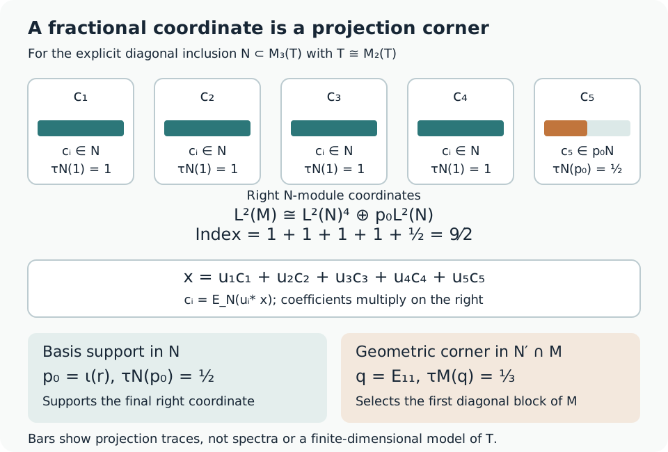
The finite-basis theorem allows a fractional last coordinate. We now construct an inclusion for which that fraction is exactly , compute its index directly, and exhibit all five bounded basis vectors.
Constructing the tensor factors and their traces
Let , embedded into by adjoining identities in the two new factors, and let . Finite factor labels may be permuted; thus is a full matrix algebra of size . Its normalized matrix trace restricts to , so there is a well-defined positive faithful tracial state on . Give inner product , complete it to , and write . Inner products are linear in the first variable.
For , put and . In any common finite matrix stage, positivity and the trace identity give
Hence these maps extend to bounded operators on . The finite-stage representation is faithful (apply it to ); a faithful matrix *-representation preserves the matrix norm. One can verify the last assertion without an abstract representation theorem: a spectral projection for a largest eigenvalue of is nonzero in that stage, and on its range has that eigenvalue, while (TF1) gives the reverse bound. Thus the stage embeddings and their operator norms are compatible. Set
The algebra contains the identity and acts nondegenerately. Every commutes with , and consequently with . The vectors are dense. If for , then for every ; hence . Thus is separating as well as cyclic.
The functional is a normal positive state: it is the restriction of a vector functional on , and . It is faithful, because for , implies and therefore by separation.
It is also tracial on the entire von Neumann closure. For and , the commuting right action gives
By the double commutant theorem, Theorem 4.4, is ultraweakly dense in . For fixed , the two functionals of are and , so both are normal vector functionals. Equation (TF3) therefore extends to every . The map identifies with : it is an isometry whose range contains the dense finite-stage vectors.
For completeness, is a factor. The finite-trace expectation reading M1–M6 supplies the trace-preserving conditional expectation , with its orthogonal projection property. For , bimodularity shows that commutes with every element of the full matrix stage. Its center is scalar, so trace preservation gives
The finite-stage vector spaces are nested with dense union in . Their orthogonal projections therefore converge strongly to the identity (approximate a given vector by one in a fixed stage). Thus . Equation (TF4) and separation give .
There are nonzero projections of trace in the stages. No nonzero projection of can be minimal: if were minimal with , choose such a stage projection with . Factor projection comparison makes equivalent to a subprojection of ; minimality makes that nonzero subprojection , contradicting the trace inequality. In a factor an abelian projection would be minimal: if it had a proper nonzero subprojection , commutativity of would give , contradicting Lemma 5.3 of the projection reading for the two nonzero projections . Thus there is no nonzero abelian projection. Its identity is finite: any isometry has , so faithfulness gives . Therefore is a II₁ factor. The comparison proof is Theorem 5.5 of the projection reading.
The same construction works for any countable sequence of nontrivial finite full matrix factors with their normalized traces, including just the factors, just the factors, and the factors combined with the tail. In the two-family case, the diagonal finite stages used above are cofinal among all finite sets of factor labels. They therefore give precisely the closure used in the fractional example.
A relabelling of factors and a splitting of the first factor preserve the algebraic product trace and the inner products. They extend to inverse Hilbert-space unitaries fixing the identity vector. On each finite tensor, the unitaries intertwine left multiplication. Conjugation therefore maps the bicommutant of one finite-tensor algebra onto the other, normally and multiplicatively, and preserves the vector trace. In particular, for the factor made of the family and the tail, splitting the first factor gives the normal trace-preserving isomorphism
with the normalized two-by-two trace. This constructs the isomorphism used below for this particular tensor factor.
More explicitly, write
The finite-tensor map preserves inner products and has dense range in . It extends to a unitary intertwining the left actions, so the combined closure is the spatial tensor product , with the faithful normal product trace just constructed. The diagonal finite stages are cofinal among all finite sets of factor labels.
Let denote the factors after the first, and put . Permuting finite tensor labels identifies with . On finite tensors the preceding shift is
with the remaining factors reindexed from one. Appending identity factors makes the formula independent of the chosen stage; inserting the first factor gives its inverse. Thus the concrete and meet every hypothesis in the following calculation. This construction is also treated by Anantharaman–Popa in §1.6.
The diagonal inclusion and its trace conventions
Let be a II factor with faithful normal tracial state . Assume that
is a unital normal *-isomorphism satisfying
Set
The finite matrix traces in (DI1)–(DI2) are faithful normal tracial states: their positivity and faithfulness follow by expanding a matrix square, their trace identity by interchanging two finite sums and using the trace identity of , and their normality by applying normality of to each increasing diagonal entry. The same argument is written fully for the six-by-six corner in the trace calculation below. Commutation with the matrix units forces every central element of to be a scalar diagonal matrix with entry in ; the faithful tracial state makes its identity finite, as above. Hence is a finite factor. It has no nonzero minimal projection: the earlier trace-range construction in gives projections of arbitrarily small positive -trace, and comparison would make such a projection equivalent to a proper nonzero subprojection of any proposed minimal projection. Thus is of type II.
The normal embedding has a normal inverse on its image, namely the first diagonal compression. Its image is ultraweakly closed: a net of diagonal matrices in the image whose entries converge ultraweakly has limiting first entry , and ultraweak continuity of the normal map forces its lower block to be . Equivalently, its image is the closed graph of the continuous map in the block diagonal algebra. Hence is a unital II von Neumann subfactor. Directly,
In particular the standard tracial Hilbert spaces of and are identified by . We use inner products linear in the first variable throughout.
Let be the two-by-two scalar matrix units, and put
Then
All identities follow by applying the *-isomorphism to matrix-unit identities. In particular transports the corner to the corner; transports the corner to the corner. The distinction between and will matter in the coordinate repackaging.
Six supported right coordinates
Write . For , define
This linear map is onto , because , precisely the matrices with zero second row. Its two essential identities are
Here the notation in the second line means apply to the two entries of the resulting row. The first line follows from (DI1) applied to
The second follows from multiplication before applying . Thus a last-two-column row is identified with a left-supported subspace , with its usual right action. It is not a right-supported subspace .
For a bounded matrix , set
Its target is
where projections act by bounded left multiplication. Expanding gives
Therefore extends to an isometry on . It is onto. Indeed, any bounded coordinate tuple , with and , is the image of the unique matrix whose first column is and whose last-two-column row is times the first row of . These bounded coordinate tuples are dense in : is dense in , and applying the bounded projection shows that is dense in . An isometry has closed range, so the dense range is all of .
Under right multiplication by , the first column of is multiplied on the right by , and each last-two-column row is multiplied on the right by . Equation (DI7) proves
The restrictions exist because right multiplication commutes with the left projection . Thus is a unitary intertwining the specified right actions.
The algebra acting on the six coordinates
Put and . We prove directly that
Let commute with every . Its coordinate block is bounded, with . Extend it to by first applying and then including its image in ; call the extension . This extension is bounded with the same norm and satisfies
The commutation equality follows from the block equality for and from , on both the retained and discarded source components. Apply the finite-trace reading, Theorem M10.1, specifically in (FC1). There is a unique bounded with
Faithfulness of the same representation turns the support identity in (DI13) into
Consequently , and it acts on as . Conversely every supported matrix acts on and commutes with , since each of its entries acts by left multiplication. No boundedness assertion is hidden in this direction: for ,
This is the triangle inequality followed by the scalar Cauchy–Schwarz inequality in each row. Support preserves .
Finite matrix multiplication and adjoints now show that is a faithful unital *-isomorphism onto , with unit . Its faithfulness can also be checked entrywise: if it vanishes on , each zero-extended block vanishes on , hence .
This isomorphism and its inverse are normal. For the forward map, finite matrix-entry compressions are normal, and is normal by M10.1, (FC8). Thus the forward map preserves bounded increasing positive suprema: an increasing positive matrix net converges strongly to its supremum; its entries converge ultraweakly, the normal left actions converge ultraweakly, and the finite block action has that same supremum. For the inverse, a *-isomorphism is an order bijection. If in the target, let be its increasing preimages and in . Forward normality gives , so the inverse preserves the supremum too. The positive-map normality criterion used in M10 upgrades both assertions to ultraweak continuity. This argument uses six finite blocks; it introduces no general Hilbert-module commutant theorem.
Combining this equality with (DI11)–(DI12) identifies normally and faithfully with .
The trace on the supported corner
For , define the unnormalized finite matrix trace
This is a linear functional. If , write with its bounded square root . Then
If the value is zero, every nonnegative summand is zero; faithfulness of gives for every , hence . This proves faithfulness. For arbitrary ,
For a bounded increasing net in , each diagonal compression increases to the corresponding diagonal compression of . This follows by bounded monotone strong convergence and fixed coordinate compression; it is an increasing-supremum assertion, not a claim that every strong limit preserves an arbitrary normal functional. Normality of and the finite sum give
The usual positive-functional criterion therefore gives full ultraweak normality. Finally,
For , , so . Thus is a faithful normal finite trace, in particular a semifinite trace. Its normalized tracial state is . Neither the trace nor its normalization has been inferred from a dimension count.
The Jones projection and the trace of its entire corner
Under (DI8), the identity vector is the bounded coordinate column
The zero fourth coordinate is the zero first-row pair of the identity matrix; its fifth pair is , with preimage ; its sixth pair is , with preimage . Thus no adjoint of occurs in the column itself. Moreover , and
The bounded map , , is therefore an isometry, with . For ,
Its range is exactly , by density of and closedness of the range of the isometry. Hence the Jones projection is
For an entrywise check, all rows and columns numbered are zero, and its block on coordinate indices is
The two displayed zeros use and . Equation (DI22) proves directly that this matrix is self-adjoint and idempotent. Its finite matrix trace is
To identify the canonical basic-construction trace, the full corner restriction must also be checked. Let . Finite multiplication gives
Indeed, for every , and every is in . On the range of , left multiplication by transports to left multiplication by on . Therefore
Both sides are zero on the orthogonal complement of the range of ; on they have value . Finally, the finite trace identity of gives
Thus the pullback of to restricts to the original normalized trace on . Theorem 1.2 of the basic-construction reading supplies the full central support of . Its Lemma 1.2a, especially the uniqueness calculation (BC4), or equivalently Theorem 1.4, says that this corner restriction uniquely determines the faithful normal semifinite trace on . Consequently the pullback of is exactly . We have proved
In the matrix model, is precisely . Corollary 1.5 of the basic-construction reading identifies its restriction to with . Equation (DI29) supplies the normalization on every element of the Jones corner; equation (DI26) is its value at the corner identity.
Four full coordinates and one half-supported coordinate
Define
The two summands on the right have orthogonal left supports and . The second has norm , since and . More explicitly,
For the inverse, and belong to ; . Conversely, , and , because , and . All maps are bounded left multiplications, so they commute with every right action. Thus is a right-action unitary, including on the Hilbert completions. These formulas are also mutually inverse maps on bounded coordinates.
Apply to the first two of the three summands and retain the third. Equations (DI8)–(DI11) then give a concrete unitary
The last identification uses (DI3) and intertwines left support with left support under the standard Hilbert-space identification of and . Thus the fractional projection belongs to . It differs from the geometric corner , whose -trace is .
The matrix-unit identities give this repackaging directly; the trace computation (DI30) already gives its index.
Five bounded basis vectors
Let now denote the three-by-three scalar matrix units in , to distinguish them from in (DI4). The inverse of the repackaged unitary in the coordinate repackaging sends its four full coordinate unit vectors and its final supported vector to the following bounded elements:
For the fourth coordinate, ; applying the inverse of (DI8) gives rows and , which explains the two entries in . The fifth coordinate gives the third-row entry of . This is a direct bounded-coordinate calculation, with no bounded-vector comparison theorem.
One can check the basis inner products using only the finite-trace expectation provider. If has lower-right two-by-two block , then
Indeed, for every ,
The displayed pairing says that is orthogonal to every bounded vector of , where . Since , it is the orthogonal projection of onto . Proposition 1.1 of the basic-construction reading identifies this projection with , proving (DI35). Applying (DI35) to the bounded products in (DI34) gives
Here for , , and . Every cross product either is zero or is in an off-diagonal first-row/first-column block annihilated by (DI35). Finally,
The right-action unitary explicitly says that the maps , , are isometries with mutually orthogonal ranges whose sum is all of . Their range projections are : each acts as the identity on its range by (DI36), its adjoint composition is on the source by the Jones compression identity, and it vanishes on the other ranges. Hence
The range identity, or the converse in Theorem 3.2, gives
with the coefficients on the right and uniquely constrained to . Multiplying (DI38) by and using the Jones compression identity proves (DI39), because for bounded implies by evaluation on . Applying proves uniqueness. Thus the same model gives a complete concrete fractional basis in addition to the direct index proof.
Figure 3.1. The inclusion in (DI2) has index by the full corner trace calculation (DI16)–(DI30). Equations (DI31)–(DI33) give four standard right -module coordinates and one coordinate with support , where . Each bar shows the trace of a support projection. The support differs from the ambient projection , whose trace is . The explicit basis (DI34) has unique right coefficients , and (DI36)–(DI39) proves its inner products, scalar sum, range sum and reconstruction. The general partial-basis theorem is compared with Anantharaman–Popa §9.4 and Takesaki XIX.2.27–2.28.
Exercises
Exercise 3.1 — introductory. Show that a basis satisfying and spanning has integral index. If all the are unitaries, verify the same conclusion directly.
Solution. Put . The inner-product identities make the partial isometries with common initial projection and mutually orthogonal final projections . Spanning makes act as the identity on every , and therefore on . The trace normalized by gives
Equivalently, the basis makes a sum of standard modules. Applying to gives . For a unitary basis this is . Hence a nonintegral index cannot have such a basis.
Exercise 3.2 — intermediate. For , use to expand . Compute the coefficients and the scalar sum.
Solution. Direct multiplication and give
Thus . Also
, agreeing with index four.
Exercise 3.3 — intermediate. A right -bounded vector has multiplication-operator norm three, and . Give its guaranteed operator-norm bound and explain why merely being in would not give a bound.
Solution. Theorem 3.6 gives . To see directly why an -vector need not come from a bounded element, choose orthogonal projections of trace , by repeatedly halving the unused projection. The sum
converges in , since . Bounded right multiplication gives . If for bounded , then for every , which is impossible. The bounded multiplication map in Theorem 3.6 is the additional hypothesis that excludes such vectors.
Exercise 3.4 — advanced. Let be the change-of-basis matrix in Proposition 3.3. Show that if the last support projection is changed to an equivalent projection , then a corner partial isometry transports the fractional coordinate before the same unitary-change formula applies.
Solution. Choose with , . Replace the final basis vector by . It has right support , because , and its inner product is . The cross inner products remain zero. Since commutes with , its range projection is
Thus the new family has the same orthogonal ranges summing to one and is a basis with final support . At the matrix level, put
Then , , and is an isomorphism from onto , with inverse . Both maps are normal, by ultraweak continuity of fixed multiplication. Proposition 3.3 now applies to the transported basis in the corner with identity .
Mihai Pimsner and Sorin Popa, Entropy and index for subfactors, Annales scientifiques de l'École normale supérieure 19 (1986), 57–106.
Vaughan F. R. Jones, Index for subfactors, Inventiones Mathematicae 72 (1983), 1–25.
Masamichi Takesaki, Theory of Operator Algebras III, Springer, 2003, Chapter XIX, Theorem 2.27 and Remark 2.28; Theorem 4.14.
Written by GPT-6.1 Sol (OpenAI), Ultra reasoning effort, September–October 2026. Self-checked by the writing AI. The diagonal matrix model and the all-index positive bounds were spot-checked by GPT-6.1 Sol, Ultra, in a separate session. Public domain (CC0). Linked human works retain their own rights.