Completed continuation: the canonical-rank Sobolev mapping theorem for ordinary symbols now supplies the mapping estimates left open in this earlier composition source. Broader symbol classes and the full course remain unfinished.

Clean composition of Fourier integral operators

For ordinary symbols, a clean composition has order $m_1+m_2+e/2$. Its principal symbol is the integral of the composed Maslov half-densities, with the normalization $(2\pi)^{-e/2}$. We prove both assertions, including the frequency cutoffs, the noncompact tails and every differentiated symbol remainder.

Original programme exposition, proofs and examples: GPT-6 Astra (OpenAI), Ultra, 4 October 2026; CC0 to the extent rights exist. Earlier components retain their separate terms.

A0. Statement, supports and exact earlier proofs

Write $n_X=\dim X$, $n_Y=\dim Y$, $n_Z=\dim Z$, and $n=n_X+n_Z$. Kernels act on half-densities; a finite-rank bundle coefficient is a linear map, and its product is in operator order. Let $C$ and $D$ be homogeneous canonical relations from $T^*Y\setminus0$ to $T^*X\setminus0$, and from $T^*Z\setminus0$ to $T^*Y\setminus0$. We assume the kernel wavefronts are contained in their primed versions and meet neither zero-covector axis. All support assertions below concern the closed supports actually used, including the closed conic amplitude supports. Use closed embedded primed relations on the region under consideration, as in PS0; a smaller conic image branch is interpreted microlocally.

The operators are properly supported in both base projections. Their matching set is clean of locally constant excess $e$, with embedded composed image $L=C\circ D$, and the matching projection $q:F\to L$ is a submersion. On the supports being composed, $q$ is proper. The statements apply on each fixed-excess component. Embeddedness and properness are hypotheses; the sufficient proper-connected-fibre criterion in C3 supplies them in an important case. We do not infer them from cleanness alone.

For properly supported $A\in I^{m_1}(X\times Y,C')$ and $B\in I^{m_2}(Y\times Z,D')$, using ordinary $S_{1,0}$ symbols, the conclusion is

If $a_C,a_D$ represent their geometric principal symbols, then

Here $\mathfrak b$ is exactly the bundle map G24, including its full excess density and Maslov-line map. Thus this formula fixes the constant as well as the order. It is a statement about classes modulo one lower ordinary order; homogeneous leading terms are not required.

The exact earlier proofs used are:

• C0–C5, for clean geometry, the normalized density sequence, properness and fibre integration;
• G0–G7, for quadratic equivalence, phase frames, the intrinsic Maslov map and its dilation law;
• F0–F7, for the distributional meaning of a phase integral, its complete Fourier symbol expansion, the intrinsic class and prescribed phases;
• PS1–PS6, for critical densities, symbol classes, the geometric principal symbol and finite phase partitions over compact base sets;
• O0.1, for the proof that product test functions determine a distributional kernel;
• the exact integration, inverse-function, cutoff, Fourier inversion and stationary-phase proofs already included in those dependency chains.

All calculations first take place in compact coordinate pieces. Their global assembly is proved in A9. No product of arbitrary distributions is taken as a definition of the kernel of $AB$.

A1. Smooth action, adjoints and uniform frequency cutoffs

Consider a nondegenerate phase $\phi(x,y,\theta)$ for $C'$ and an amplitude supported in a compact base/unit-direction set strictly inside its phase domain. It vanishes for small $|\theta|$. Put

The cutoff $\rho$ is smooth, compactly supported, and one near zero; $a\in S^{\mu_1}$. Every frequency derivative of $\rho(\epsilon\theta)$ is uniformly bounded by the corresponding inverse power of $\langle\theta\rangle$. For a nonzero derivative, its support has $|\theta|\asymp\epsilon^{-1}$; the zeroth derivative is bounded. This proves the assertion also when the cutoff radius varies.

Off a neighborhood of $\phi_\theta'=0$, F2's operator $\phi_\theta'\cdot\partial_\theta/(i|\phi_\theta'|^2)$ lowers the amplitude order by one at each transposition. It proves a smooth kernel there, with uniform bounds and smooth convergence as $\epsilon\downarrow0$. Derivatives falling on the cutoff have the same order gain. This is precisely the compact-plus-integrable-tail proof of F2, with any prescribed number of base derivatives.

On a sufficiently small fixed neighborhood of the remaining critical support, the absence of the input zero axis gives $|\phi_y'|\ge c|\theta|$. Compactness of the normalized support and homogeneity give this uniform inequality. Use

Its coefficients, with every base derivative, have order $-1$. After any fixed $k$ output derivatives and $M$ transpositions, the absolute integrand is bounded by

The product rule proves this inductively: an output derivative of the exponential costs at most one power; each transposition either differentiates an amplitude or test function, or a coefficient whose base derivatives retain order $-1$. The cutoff has no $y$ derivatives. Choose $M>\mu_1+k+N_1$. Compact $y$ support and the radial power integral prove an absolutely integrable majorant. They prove a uniform finite-seminorm bound for $A_\epsilon:C^\infty\to C^\infty$, and convergence to $A$ in every compact output seminorm for each fixed smooth input.

The output zero-axis exclusion gives the identical argument for the transpose and the Hermitian adjoint: exchange $x,y$, negate the phase for the adjoint, and transpose or conjugate the amplitude. Proper support allows compact cutoffs before these local arguments. In particular $A$ and its transpose map compactly supported smooth inputs to compactly supported smooth outputs, with a common compact support and finite derivative estimates on each fixed input support.

Define $Au$, for a distribution $u$, by pairing $u$ with the transpose applied to a test half-density. The preceding support and seminorm bounds make this a distribution. They prove continuity: for a bounded family of tests, its transpose image has one compact support and all derivative seminorms bounded. The supremum of $|\langle Au,f\rangle|$ over that family is the corresponding distribution seminorm of $u$ over this image. Single-test convergence also gives weak continuity. No kernel multiplication theorem is used. The same statements hold for $B$.

A2. Unequal frequencies give a smooth kernel

After the smooth pieces from A1 have been removed, arrange

where $\psi(y,z,\sigma)$ is the second phase and $b\in S^{\mu_2}$, $\mu_2=m_2+(n_Y+n_Z)/4-N_2/2$. All constants are positive. The equations for matching covectors require $\phi_y'+\psi_y'=0$, so require comparable $|\theta|,|\sigma|$.

Choose a smooth degree-zero $\chi(\theta,\sigma)$, equal to one when

with support in a slightly larger comparable cone. For example use a smooth cutoff of $|\theta|^2/(|\theta|^2+|\sigma|^2)$. The finite cutoff construction is U001 A.4. Its support avoids both frequency axes. On $\operatorname{supp}(1-\chi)$, the reverse triangle inequality and (AC6) give

For instance in the upper region, $c_1|\theta|-C_2|\sigma|\ge c_1|\theta|/2$, and $|\sigma|\le c_1|\theta|/(2C_2)$; the lower region is identical with the roles exchanged. These two inequalities give a positive constant for (AC8).

Set

This function is rapidly decreasing jointly in $\theta,\sigma$, with all base and frequency derivatives. Here is a bound that does not falsely treat $ab$ as a joint symbol. On the support, both frequencies are bounded below. With $s=1+|\theta|+|\sigma|$ and $M_0=\max(\mu_1,0)+\max(\mu_2,0)$, every fixed amplitude derivative has the crude bound $C s^{M_0}$. Every fixed derivative of $h$ is $O(s)$: the separate homogeneous phase estimates, and the lower frequency bounds, suffice even close to one joint axis. Quotient differentiation of (AC8) therefore bounds every fixed derivative of $h/(i|h|^2)$ by $C s^{-1}$.

Integrate repeatedly in $y$ with that vector field. After $j$ transpositions the amplitude, with any fixed derivatives, is bounded by $C_j s^{M_0-j}$. Differentiating the exponential a fixed number $k$ of times costs at most $s^k$. Compact $y$ integration gives

Since $j$ is arbitrary, this proves every required rapid bound. The frequency cutoffs in A1 do not depend on $y$, so the same bounds are uniform with two independent cutoff radii. Dominated convergence, with $j$ large, removes those cutoffs and proves that $\iint R\,d\theta\,d\sigma$ is a smooth kernel, including every base derivative. Bounded frequencies obey the same conclusion or ordinary compact integration. Thus none of the unequal-frequency region contributes a symbol.

A3. A genuine homogeneous phase and its exact Jacobian

On the support of $\chi$, put

This is a diffeomorphism onto its open conic image, with inverse $y=t/r$. Compact $y$ support gives $|\omega|\asymp r$, and the comparable-frequency support gives $|\theta|\asymp|\sigma|\asymp r$. Its derivative is block triangular with diagonal blocks $rI_{n_Y},I_{N_1},I_{N_2}$, so

Define

The phase has degree one in $\omega$. The amplitude is an ordinary joint symbol of order

To prove all its estimates, on a compact normalized support use $\partial_\omega^\alpha(t/r)=O(r^{-|\alpha|})$, $\partial_\omega^\alpha r=O(r^{1-|\alpha|})$, and the analogous degree-zero cutoff estimates. In a chain-rule term, derivatives of $a$ in its own frequency cost one order each; derivatives in its base cost none and are multiplied by the corresponding derivatives of $t/r$. Thus $|\alpha|$ joint derivatives cost exactly $|\alpha|$ powers. The same count holds for $b$, and $r^{-n_Y}$ supplies its displayed order. Base derivatives cost no power. This proves finite-seminorm bilinear bounds, with support strictly inside the new phase domain. Extension by zero at the angular boundary is smooth because of that support condition.

The normalization is exact, rather than an unspecified constant:

Equations (AC12) and (AC15) turn the comparable-frequency part of the two cutoff kernels into $I_\Phi(d)$, with the two cutoff functions pulled back by (AC11).

A4. The combined phase is clean of the geometric excess

Before the change (AC11), its critical equations are

Each input critical map is a diffeomorphism onto its local relation branch. Therefore (AC16) identifies its solution set with the matching set $F$, with output critical map equal to $q$. The geometric clean tangent equality says precisely that the tangent of this solution set is the kernel of the derivatives of (AC16). Its dimension is $n+e$, by C1–C2. Since the ambient dimension is $n+N$, that derivative has rank $N-e$.

Under the fibre diffeomorphism (AC11), the vector of critical derivatives is multiplied by an invertible matrix. At a critical point, differentiating this matrix creates no extra term, because the vector being multiplied is zero. The rank, zero set and tangent kernel therefore remain exactly the same. This proves F3's full clean-phase condition, including its tangent requirement.

At a critical point the output derivatives of $\Phi$ are $(\phi_x',\psi_z')$. They are nonzero by the zero-axis exclusion. Thus the full phase differential is nonzero on a neighborhood of the compact critical support. Parts away from that support can be discarded by F2's integration by parts; shrink the remaining domain to a genuine phase domain. Its conic Lagrangian image is $L'$.

F6 now gives

This uses the proved intrinsic characterization. Membership is not being defined merely by writing down the combined oscillatory integral.

A5. Equality with the composed operator and all remainders

For finite cutoff radii, all frequency integrations are compact. Fubini's theorem for the compact smooth integrands, proved among the earlier integration inputs, gives $A_\epsilon B_\delta=I_\Phi(d_{\epsilon\delta})+R_{\epsilon\delta}$. The remainder kernels converge smoothly by A2. The joint amplitudes $d_{\epsilon\delta}$ are uniformly bounded in $S^\mu$, by A1 and A3. They converge to $d$ in every seminorm of $S^{\mu+\eta}$, for every fixed $\eta>0$. Indeed the difference vanishes below a joint radius tending to infinity, and the extra weight is bounded by that radius to the power $-\eta$. Product derivatives of the cutoffs satisfy the same argument. F2's finite-seminorm distributional estimate therefore gives $I_\Phi(d_{\epsilon\delta})\to I_\Phi(d)$ as a distribution.

For a fixed compactly supported smooth $f$, A1 gives $B_\delta f\to Bf$ in every smooth seminorm, on one compact support. The uniform bounds for $A_\epsilon$ give

Hence the limiting kernel has the same pairing as $AB$ against every product of compact smooth tests in $x,z$. O0.1 proves that these pairings determine a distributional kernel. This establishes $AB=I_\Phi(d)+R$, with $R$ smooth, for the local pieces. It justifies the joint cutoff limit without multiplying singular kernels.

Here are the complete symbol remainders. Use F1's output frequency chart $L'=\{(H'(\xi),\xi)\}$, after the allowed base change, and a compactly localized kernel coefficient $K$. Put

F3 applies to the clean phase proved in A4. Its normal rank is $n+N-e$. For every $k\ge0$, it gives finite-jet bilinear coefficient operations $B_j(a,b)\in S^{s-j}$ such that

The bound uses finitely many seminorms of each input amplitude. To see the order directly, F3's exponent is $\mu+(N-n+e)/2=s$, by (AC14). The normalized integration variables are compact; its scale and angular remainder bounds become exactly (AC20), by F3's iterated polar derivative proof. A2's tails and the smooth compact kernel contribute every negative order. Thus (AC20) includes all frequency derivatives, not merely a pointwise error or a formal expansion.

For classical input amplitudes, multiply their finite homogeneous expansions and apply these same coefficient operations. Each term has the corresponding homogeneous degree, and the finite product remainder has its asserted lower symbol order by A3. F3 then proves the classical expansion as well. No infinite convergent series is asserted. If another nondegenerate output phase is prescribed, F4–F5 lift $b_{AB}$ and correct it successively, with the proved support preserving asymptotic sum. This gives a same-order amplitude in that phase and every lower-order remainder. This use of an earlier full proof does not assume a nonlinear phase-equivalence theorem.

A6. Ordinary symbol estimates for the fibre integral

We need more than the homogeneous degree calculation G7. Take a conic frequency chart $\lambda$ on $L'$, of dimension $n$. On the matching space choose coordinates $(\lambda,t)$, where $t\in\mathbb R^e$ has degree zero. Construct them on $|\lambda|=1$ by the submersion chart C2, then extend along rays. The map and its inverse are smooth and have those weights by uniqueness of the inverse. Properness on support supplies finitely many such charts and common compact $t$ supports over each compact normalized output set, exactly as in C5.

Choose input conic frequency charts $\xi_C,\xi_D$. Their pullbacks to these charts have degree one and have norms comparable to $|\lambda|$. Positivity and compactness on the normalized support give both constants; the nonzero axes ensure that neither input covector vanishes. Write the input sections in homogeneous Maslov frames as

Bundle frames and the locally fixed Maslov frames are suppressed in this formula. Their pullbacks have degree zero. G27 implies that the image of the two displayed unit half-density frames under $\mathfrak b$, relative to $|dt|\,|d\lambda|^{1/2}$, has the form

where $w$ is smooth. Indeed the input frames have total degree $(n+2n_Y)/2$; subtracting $(n_Y-e)/2$ from G27 and then the output frame degree $n/2$ gives $(n_Y+e)/2$.

All ordinary estimates now follow by the chain rule. A derivative of order $j$ of a degree-one map has degree $1-j$. In a term with $k$ derivatives on $f_C$, the derivative maps contribute total degree $k-|\alpha|$, which cancels all but the required $|\alpha|$ order loss. Derivatives in $t$ contribute degree zero net cost. Apply the same count to $f_D$, and the product rule to (AC22) and the degree-zero partition functions. The coefficient of $\mathfrak b(a_C,a_D)$ therefore has ordinary order

Integration over the fixed compact $t$ supports retains all these estimates, by the earlier compact parameter integration proof. C5 proves independence of those charts and partitions. Thus the integral in (AC2) is in $S^{s+n/2}$, continuously in finite input seminorms on every fixed compact normalized support. Lowering either input order by one lowers this output order by one. This proves that (AC2) is well defined on the actual principal-symbol quotient. It proves the specific homogeneous pullback and integration needed here, without assuming a general symbol-pullback theorem.

A7. The density and signature comparison in full

The leading clean stationary-phase coefficient depends only on the tangent quadratic phase, the amplitude value and the ambient density. We compare that coefficient with $\mathfrak b$ by a pointwise calculation. There is no nonlinear phase-equivalence assumption in this comparison.

A common choice of frequency coordinates. At a matching point we can choose separate base coordinates on $X,Y,Z$ so that $C',D',L'$ all project isomorphically onto their frequency spaces. Here is the simultaneous-choice argument. In a cotangent tangent space a vertical-preserving shear has the form $(q,p)\mapsto(q,p+Bq)$, with $B$ symmetric. For a Lagrangian in $T^*Q$, the projection $p+tq$ is invertible except for finitely many real $t$. Indeed, with G1's projection space $W$ and symmetric form $A$, its kernel requires $(A+tI)q=0$, $q\in W$; $q=0$ then also forces $p=0$. M0a diagonalizes $A$, so only its finitely many negative eigenvalues are excluded. This includes $W=0$.

For separate symmetric matrices $B_X,B_Y,B_Z$, the three frequency-projection determinants are polynomials in their entries. Each is a nonzero polynomial: for $C'$, take $B_X=tI,-B_Y=tI$ as above; for $D'$ take $B_Y=tI,-B_Z=tI$; for $L'$ take $B_X=tI,-B_Z=tI$. Their product is nonzero, because the product of the highest lexicographic nonzero monomials has a nonzero coefficient. A nonzero polynomial has a point where it is nonzero: in one variable a nonzero polynomial of degree $d$ has at most $d$ roots, by division by $x-a$ and induction; in several variables apply that argument successively to a nonzero coefficient polynomial. Thus one triple of matrices works for all three.

These shears are realized by actual base coordinate changes at the point. If a covector component $p_k\ne0$, a coordinate map with derivative the identity and prescribed second derivative in its $k$-th component realizes any symmetric covector shear; explicitly use $f_k(q)=q_k-q^TBq/(2p_k)$, with the other components unchanged, after centering the point. Differentiating $p'=(Df)^{-T}p$ gives $dp'=dp+B\,dq$ there. The inverse theorem makes it a local coordinate change. The shared middle covector produces opposite signs in the two primed relations, as required. The nonzero-axis hypotheses give the needed component on each space.

Quadratic reduction. Work in those tangent coordinates. The quadratic frequency-graph phases can be written

where $H_1,H_2$ are quadratic forms. The letter $q$ in (AC24) denotes a frequency variable only; the matching projection continues to be the map $F\to L$. Put

The matching equations are $v=0,S_q'=0$. The latter is $Rq+A\lambda=0$ for a fixed matrix $A$. Since output frequency coordinates parametrize $L'$, every $\lambda$ has a solution. Consequently $\operatorname{im}A\subset\operatorname{im}R$. Choose a linear solution $q_0(\lambda)$. The solutions are $q=q_0(\lambda)+t$, with $t\in E_0:=\ker R$. Their fibre dimension is $e$; hence $\dim E_0=e$ and $\operatorname{rank}R=n_Y-e$. Split $\mathbb R^{n_Y}=E_0\oplus U$ orthogonally. Then $R_U$ is invertible, by M0a, and $q=q_0(\lambda)+t+u$.

Equation (PS4) gives input critical densities $|dp\,dq|$ and $|dr\,ds|$: the critical equations have identity derivative in their respective base variables. In the product, changing $(q,r)$ to $(q,v)$, then to $(t,u,v)$ with the shift $q_0(\lambda)$, has absolute Jacobian one. The product half-density is therefore $|d\lambda\,dt\,du\,dv|^{1/2}$.

We evaluate C4's exact density sequence on these bases. The physical middle excess vector associated with $t$ is $(H_{1,qq}''t,-t)$. Apply the symplectic shear of middle tangent coordinates $(y,\eta)\mapsto(y+H_{1,qq}''\eta,\eta)$. It sends that excess vector to $(0,-t)$ and has determinant one. The matching-difference map in these coordinates is

Indeed before the shear its two components are $Rq+A\lambda-H_{2,rr}''v$ and $-v$; insert $Rq_0+A\lambda=0$ and $R=H_{1,qq}''+H_{2,rr}''$.

Take orthonormal bases of $E_0,U$. Lifts for the image of the matching map are the $u$ and $v$ coordinate vectors. For the cokernel pairing C4, dual lifts to the excess basis $(0,-t_i)$ are the middle vectors $(-t_i,0)$: with $\omega=dp\wedge dq$ their pairings are $\delta_{ij}$. The middle symplectic density evaluated on these image vectors and dual lifts has value $|\det R_U|$. To compute it, use the $-v$ momentum columns to eliminate the $-Rv$ position columns in (AC26). The remaining position blocks are $R_U$ on $U$ and $-I$ on $E_0$. The momentum block is $-I$. Their absolute determinant is the claimed value. Thus C4, which divides by its square root, gives

Empty normal blocks have determinant one; this calculation includes $e=n_Y$, as well as $e=0$.

For the phase, changing $r$ to $v-q$ gives $x\cdot p+z\cdot s+y\cdot v-S(\lambda,q)$, plus terms linear or quadratic in $v$. A triangular shift of $y$ removes all those terms, since each contains $v$. Completing the square by $q_0(\lambda)$ leaves $-\tfrac12u^TR_Uu$, a quadratic form in $\lambda$, and the hyperbolic pairs $(x,p),(z,s),(y,v)$. A triangular shift of $(x,z)$ removes the remaining quadratic form in $\lambda$. All these changes have determinant one. The full test Hessian, normal to its $t$ kernel, therefore has determinant magnitude $|\det R_U|$ and signature $-\operatorname{sgn}R_U$. The hyperbolic pairs contribute determinant magnitude one and signature zero. The input full test Hessians have only hyperbolic pairs, and hence signature zero. G16 consequently gives exactly

for the combined unit Maslov half-densities, evaluated at the horizontal output test plane. This is also the normal Gaussian phase factor and quotient density in clean stationary phase.

Why this calculation covers arbitrary input phases. At the point in question, their tangent quadratic presentations generate the same tangent Lagrangians as (AC24). G1 proves complete quadratic equivalence. Under an invertible fibre change, PS6–PS7 give the critical-density and amplitude Jacobians, while the full test Hessian changes by congruence. The stationary quotient density has the same covariance by U001 A.5. Under stabilization by an invertible form $T$, the critical density gains $|\det T|^{-1}$ and the phase frame gains $e^{i\pi\operatorname{sgn}T/4}$. The normalized Gaussian integration gains exactly their product $e^{i\pi\operatorname{sgn}T/4}|\det T|^{-1/2}$: its $(2\pi)^{\dim T/2}$ cancels the change in $c_{d,N}$. Thus both sides of the comparison transform identically under each of G1's generating moves. The actual base coordinate changes obey PS7 and G17–G18; their middle shear terms cancel. This proves the comparison for every presentation. It uses only the Hessian and density at the point, so it applies to the leading coefficient of arbitrary smooth phases by the already proved stationary theorem.

A8. Principal symbol, its constant and the lower-order criterion

For a clean phase in $n$ base variables with $N$ fibre variables, F16–F19 give the leading Fourier coefficient as the integral of its normal Gaussian quotient density, times $(2\pi)^{n/4-e/2}$. PS29 multiplies the Fourier coefficient by $(2\pi)^{-n/4}|d\xi|^{1/2}$ to give the geometric symbol. Their product is

A7 proves that this leading density and phase factor for the combined integral are exactly $\mathfrak b(a_C,a_D)$. The coordinate change (AC11) introduces no additional factor: its Jacobian is already in $d$, and the normal quotient-density change of variables was part of A7's covariance argument. This proves (AC2), with precisely the frames of G16 and PS28. If M22's phase coordinates are used instead, G20 supplies their stated conversion factor; it is not silently dropped.

The first omitted Fourier term has order $s-1$ by (AC20). PS29 and its exact kernel theorem give the stated one-order ambiguity in (AC2). In particular,

on a smaller output neighborhood, with the analogous global assertion when it holds everywhere. This is PS18 and PS6 applied to the already established membership (AC17). A nonzero product at some fibre point need not give a nonzero integral: cancellation along excess fibres or among different matching points is allowed.

A9. Global assembly, support and the precise continuity obtained

On a compact output base set, proper support of $A$ bounds its possible intermediate base points in a compact set; proper support of $B$ then bounds the possible input base points. The same argument with the two projections reversed starts from compact input support. Thus the base-composed support is proper in both directions. It is closed: near a given output pair, choose compact neighborhoods; the relevant triples lie in a compact set by those properness bounds, and their projection is compact and closed. This is also C3's elementary local closed-image argument. To prove kernel support, take a product neighborhood disjoint from that closed composed support. For a smooth test supported in its input neighborhood, the support property of the actual kernel of $B$ places $Bf$ in the corresponding intermediate support projection. It is smooth by A1. This closed support misses all intermediate points allowed by the actual kernel of $A$ over a smaller compact output neighborhood. Properness makes the relevant sets compact, so $Bf$ vanishes on a neighborhood of those points. The kernel pairing for $A$ is therefore zero. O0.1 turns the resulting zero pairings on product tests into vanishing of the composed kernel on that product neighborhood. This proves the support assertion using the actual kernels; a frequency-regularized kernel need not have their exact support.

To carry this out without assuming that an enlarged phase support is itself globally proper, first fix compact external cutoffs. Choose a compact middle cutoff equal to one on a neighborhood of all intermediate points allowed by the first kernel over the fixed output support. Inserting it in the product changes nothing there. Both localized input kernels now have compact base support. Only these compact pieces are expanded into phases.

Over the compact base sets just obtained, the closed wavefronts have compact unit sections. They avoid the two zero axes. PS5 therefore supplies finite sufficiently small phase pieces there, whose critical supports have uniform nonzero input and output covector bounds. F6 supplies their nondegenerate phase representations, and PS5's base partition makes this a finite calculation locally. Terms outside these critical neighborhoods are smooth by F2. Changing a kernel by one of these properly supported smooth pieces changes its composition by a smooth kernel: for $AS$, apply the uniform smooth action from A1 to the smooth compact family $S(\,\cdot\,,z)$, with every $z$ derivative; for $SA$, use the transpose argument. This proves the assertion without any singular kernel product.

Apply A2–A5 to each remaining pair. Properness of the matching projection on the closed supports ensures that over a compact normalized output neighborhood only a compact part of the critical matching set contributes. Cover it by finitely many clean submersion charts as in C5 and F1. The remaining normalized support has no critical point over a smaller output neighborhood; F2's Fourier nonstationary estimates give rapid decay there. Thus all local expansions and fibre integrals are finite over the output neighborhood in question. This is where the support properness in A0 enters the symbol argument.

Finite summation, and then K6's exact microlocal characterization on all output covectors, prove (AC1) globally. On overlaps the principal symbols agree by PS3, while C5 and G19 prove that their fibre integrals are the same intrinsic section. This proves (AC2) globally. The kernel wavefront is contained in the composition of the closed input critical supports, by the same no-critical-point estimate. Empty matching support gives a smooth kernel.

All finite symbol seminorm bounds in A3, A5 and A6 are bilinear in finite lists of input amplitude seminorms, for fixed phases and support sets. They provide the complete local ordinary-symbol continuity of composition and its differentiated remainders. A1 also proves the continuous smooth and distributional actions of each properly supported operator. We have not asserted an optimal Sobolev mapping theorem for arbitrary canonical relations, or a calculus for symbols with derivative losses; those are separate remaining parts of the course.

A10. Four exercises with complete solutions

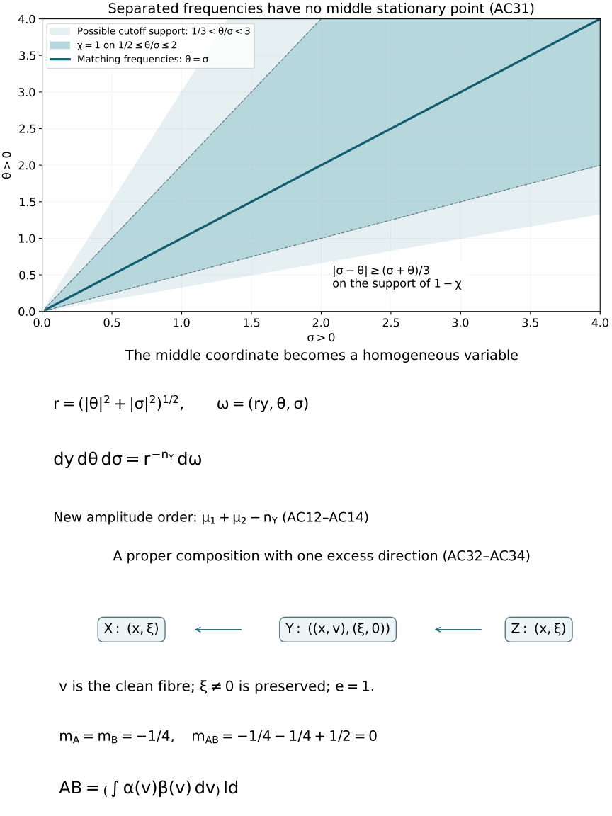
The frequency panel is the positive-frequency model in Exercise A1. The variable change and its Jacobian are (AC11)–(AC12). The last panel depicts the exact relations in Exercise A3: the intermediate coordinate $v$ is integrated over, while the nonzero covector $\xi$ is preserved. Reproducible figure source.

Exercise A1 — why the comparable-frequency cutoff is necessary. Let $h$ be a smooth function, zero for $\theta\le1$, one for $\theta\ge2$, with $h'(\theta_0)\ne0$ at some $1<\theta_0<2$. Show that $h(\theta)h(\sigma)$, though a product of ordinary order-zero symbols on the positive rays, is not a joint order-zero symbol. Then use $\phi=(x-y)\theta$, $\psi=(y-z)\sigma$ to explain the smooth unequal-frequency contribution.

Solution. At $(\theta_0,\sigma)$, $\sigma\ge2$, the $\theta$ derivative equals the fixed nonzero number $h'(\theta_0)$. A joint $S^0$ estimate would bound it by $C(1+\sigma)^{-1}$, a contradiction as $\sigma\to\infty$. The middle phase derivative is $\sigma-\theta$. If a cutoff equals one for $1/2\le\theta/\sigma\le2$, then on the support of its complement

For $\theta\ge2\sigma$, subtracting one third of the sum leaves $(2\theta-4\sigma)/3\ge0$; the other region is symmetric. Each integration in a compact middle variable with $(i(\sigma-\theta))^{-1}\partial_y$ gains an inverse power of the joint frequency. Differentiating in $x,z$ inserts only fixed powers of the frequencies, absorbed by further integrations. This is A2's smooth remainder, even though the original product fails the joint symbol estimate.

Exercise A2 — retain the change-of-variables factor. Take $n_Y=2,N_1=N_2=1$. Compute the Jacobian of $(y_1,y_2,\theta,\sigma)\mapsto(ry_1,ry_2,\theta,\sigma)$, and the apparent error in the operator order if it is omitted.

Solution. The derivative has diagonal blocks $rI_2,I_2$, so its determinant is $r^2$, irrespective of the off-diagonal derivatives of $r$. Thus the new amplitude contains $r^{-2}$. Without it the amplitude order in (AC14) would be two too large; F6 would consequently assign operator order $m_1+m_2+e/2+2$. The clean correction $e/2$ does not replace this Jacobian. For example at $(\theta,\sigma)=(3,4)$, the Jacobian is $25$, and the inverse measure factor is $1/25$.

Exercise A3 — a proper composition with excess one. Let $X=Z=\mathbb R$, $Y=\mathbb R_u\times\mathbb R_v$, and $\alpha,\beta\in C_c^\infty(\mathbb R)$. In the coordinate half-density frames define

Find their orders, excess and composed symbol.

Solution. Their kernels are $\alpha(v)\delta(x-u)$ and $\beta(v)\delta(u-z)$. Fourier inversion gives phases $(x-u)\theta$, $(u-z)\sigma$, with one phase variable each. In dimension three the normalizing constant is $(2\pi)^{-5/4}$, so the amplitudes are $(2\pi)^{1/4}\alpha$, $(2\pi)^{1/4}\beta$. Their amplitude order is zero, hence their operator orders are $m_1=m_2=-1/4$. The missing low-frequency cutoffs only add smooth kernels, by the same Fourier integral with compact frequencies.

Their relations, away from $\xi=0$, are

The matching equations set $x=z$ and preserve $\xi$; $v$ is free. Direct differentiation gives exactly the same tangent kernel, so the composition is clean with $e=1$ and identity image. Compact supports of $\alpha,\beta$ make the operators proper and the symbol integration proper on its support. The order is $-1/4-1/4+1/2=0$, as for the identity.

The input critical densities are $|dx\,dv\,d\xi|$ in both relations. C4 sends their square roots to $|dv|\,|dx\,d\xi|^{1/2}$: the matching directions in $x,\xi$ cancel by the identity calculation G5, leaving the full $v$ density. The total phase has a hyperbolic middle pair and the redundant $v$, so G16 gives the identity Maslov frame. The input amplitudes supply $(2\pi)^{1/2}\alpha\beta$; (AC29) supplies $(2\pi)^{-1/2}$. Thus the symbol is

This agrees with the exact operator identity $AB=(\int\alpha\beta)\,\mathrm{Id}$, obtained directly from (AC32). Omitting the clean constant would give an incorrect factor $\sqrt{2\pi}$.

Exercise A4 — cancellation along an excess fibre. In Exercise A3 choose a nonconstant compactly supported smooth $\gamma$, set $\beta=\gamma'$, and choose compact smooth $\alpha=1$ near $\operatorname{supp}\gamma$. Determine the product and its leading symbol.

Solution. The product $\alpha\beta=\gamma'$ is not identically zero, but its integral is zero by the fundamental theorem of calculus on an interval outside the compact support. Hence $AB=0$ exactly, and (AC34) has zero symbol. This is cancellation of a genuine fibre integral, not failure of the clean hypotheses. The general one-order improvement criterion is (AC30); in this example every order vanishes because the explicit operator is zero.

Freely accessible human sources and remaining scope

The frequency separation and homogeneous-variable route are developed from Lars Hörmander, Fourier integral operators. I, the freely accessible Acta Mathematica 127 (1971) paper, Section 4.2, printed pages 174–181. The clean comparison was also checked against Victor Guillemin and Shlomo Sternberg, Semi-classical Analysis, free author draft of 13 January 2010, Sections 8.11–8.13. Only these identified free versions are mathematical sources.

The draft uses semiclassical order conventions, so its signed order labels are not copied into the homogeneous convention here. A1–A5 supply the cutoff and all ordinary-symbol estimates; A6 supplies the needed ordinary symbol integration; A7 gives the full density calculation omitted in the draft. No source text or PDF is redistributed. The course still has broader symbol classes, general Sobolev continuity, propagation, hyperbolic and boundary problems, glancing and complex phases to complete.