Subanalytic triangulations on analytic manifolds

This reading constructs compatible locally finite triangulations of arbitrary Hausdorff second-countable real analytic manifolds. It supplies the relative Euclidean construction, elementary finite-colour chart covers, differentiable subanalytic cutoffs, a proper embedding and analytic recovery of the transported open simplices. Six exercises have complete solutions.

Original teaching text and solutions by GPT-6.1 Sol (OpenAI), Ultra, October 2026. CC0.

Setting and dependency boundary

Manifolds have finite dimension and no boundary. The prescribed family is locally finite, and each member is locally subanalytic. The compatible analytic partitions and simultaneous constant-rank refinements are proved below from the linked finite-cell calculus and compact chart covers. The relative construction retains lower subanalytic uniformization and analytic regularity prerequisites, together with analytic Noetherianity, the analytic constant-rank theorem and differential-equation facts, including uniform uniqueness. The dimension and frontier results have their complete linked provider below. Those lower results remain separate prerequisites. The finite-colour cover and cutoff proofs do not assume a triangulation or a covering-dimension theorem.

The bounded-chart comparison and global Boolean/projection calculus used for proper images have their complete written provider in analytic finiteness and preparation. That separately licensed component retains Guillaume Valette’s credit and its reuse terms; its expression is not imported here.

Compatible locally finite analytic partitions

The finite analytic cell theorem, its Boolean and projection calculus, and its bounded-chart comparison give the following manifold partition. The compact chart-ball refinement is proved below in Section 2 of the cutoff construction. These are the exact inputs; no analytic regular-locus theorem or uniformization theorem is needed for this partition.

Partition theorem. Let $M$ be a finite-dimensional Hausdorff second-countable real analytic manifold without boundary, and let $\{A_a\}_{a\in I}$ be a locally finite family of locally subanalytic subsets. There is a countable locally finite partition of $M$ into connected locally subanalytic embedded analytic submanifolds compatible with every $A_a$: each partition member is contained in or disjoint from each $A_a$. Given finitely many analytic maps $f_j:M\to N_j$ to real analytic manifolds, the partition can also make every restriction $f_j|_S$ have constant rank.

Compact chart pieces and compatibility

The compact exhaustion and shell construction in the linked cutoff proof supplies a countable cover by open coordinate balls $B_i$ with compact closures $L_i=\overline{B_i}$ contained in analytic charts; the family of these closures is locally finite. For instance, use the inner balls in that construction: their closures are contained in its locally finite outer compact balls. Each ball and its closure is locally semianalytic. In its chart it has a squared-norm inequality, and outside its compact closure it is empty on a neighborhood. The exhaustion sets need not be subanalytic; only the selected balls enter the partition.

For the map assertion apply this refinement to the open cover consisting of intersections of a source chart and inverse images of target charts for the finitely many $f_j$. Thus each $L_i$ lies in one source chart, and every $f_j(L_i)$ lies in one selected target chart. The source and target coordinate images of these compact sets are bounded. The maps in these coordinates are analytic on a neighborhood of $L_i$.

Every compact set meets only finitely many members of a locally finite family. Indeed, cover the compact set by finitely many neighborhoods, each meeting finitely many family members; combine their finite lists. In particular $L_i$ meets only finitely many $L_k$ and finitely many nonempty $A_a$.

Enumerate the balls and put

$$E_i=B_i\setminus\bigcup_{k<i}B_k. \qquad\text{(P1)}$$

These sets are disjoint and cover $M$, because each point has a first containing ball. For fixed $i$ the earlier union is finite; its trace near $L_i$ uses only the finitely many earlier closures that meet a sufficiently small neighborhood of $L_i$. To justify that neighborhood, first take a finite cover of $L_i$ by neighborhoods meeting only finitely many closures, then discard the finitely many closures missing $L_i$ by shrinking around that compact set. Thus $E_i$ is a finite Boolean combination of locally semianalytic balls near $L_i$. The local Boolean calculus also makes every relevant $A_a\cap E_i$ locally subanalytic there.

In the chosen source coordinates, these traces are bounded and locally subanalytic at every point of their ambient closures. Their closures lie inside the compact coordinate image of $L_i$, strictly inside the source chart. Extension by the empty set therefore creates no chart-boundary obstruction. The proved bounded-chart comparison makes $E_i$ and all the finitely many relevant $A_a\cap E_i$ globally subanalytic in this Euclidean space.

Apply the finite analytic cell theorem compatibly with these sets, and keep just the cells in $E_i$. Each kept cell is a connected embedded analytic submanifold. Its global subanalyticity gives local subanalyticity in the source chart, including at points of its closure; compact containment gives local emptiness outside that chart. It is therefore locally subanalytic in $M$. It lies in or misses every $A_a$, including those whose trace on $L_i$ is empty.

There are finitely many kept cells for each $i$, and each is contained in $L_i$. A neighborhood meeting only finitely many $L_i$ consequently meets only finitely many kept cells. They give a countable locally finite partition of $M$. This proves the first assertion. It uses local finiteness of the compact closures; a merely countable atlas does not supply that conclusion.

Analytic coordinates on a cell

We spell out the cell coordinates needed for rank refinement. A cylindrical analytic cell $C$ of dimension $d$ has a coordinate projection $q:C\to V$ which is a definable analytic diffeomorphism onto an open definable $V\subset\mathbb R^d$. Keep precisely its band coordinates and discard its graph coordinates.

This follows by induction through the cylindrical construction. For a graph over a cell with inverse parametrization $\phi$, use $u\mapsto(\phi(u),\zeta(\phi(u)))$; the old free-coordinate domain remains open. For a band over that cell, the new free domain is

$$\{(u,t):u\in V,\ \zeta_-(\phi(u))<t<\zeta_+(\phi(u))\}. \qquad\text{(P2)}$$

It is open because the endpoints are continuous, omitting the corresponding inequality for an infinite endpoint. Its inverse parametrization is $(u,t)\mapsto(\phi(u),t)$. These maps and their inverses are analytic. Their graphs are definable by the graph, composition and projection calculus; hence the domains are definable too. In dimension zero use the single point $\mathbb R^0$. This proves the coordinate assertion, including the analytic embedding and its inverse, directly from the cell definition.

Definable derivatives and restriction ranks

Fix a kept cell $C\subset E_i$, and write $\phi:V\to C$ for this inverse parametrization. In the chosen target coordinates the maps $g_j=f_j\circ\phi$ are analytic and definable. To check the latter assertion, the coordinate graph of $f_j$ over $L_i$ is bounded and locally semianalytic at every point of its compact closure: its defining analytic equation is valid on a neighborhood of $L_i$, and the closed coordinate ball supplies the domain condition. The bounded-chart comparison gives a globally subanalytic graph. Restriction to $C$ and composition with $\phi$ preserve definability.

For a scalar analytic definable $g:V\to\mathbb R$, the derivative graph, with $u\in V$, is described by

$$\begin{aligned} v=\partial_\ell g(u) \quad\Longleftrightarrow\quad &\forall\epsilon>0\ \exists\delta>0\ \forall h\in\mathbb R,\\ &\bigl(0<|h|<\delta\ \text{and }u+he_\ell\in V\bigr)\\ &\hspace{1em}\Longrightarrow \left|\frac{g(u+he_\ell)-g(u)}h-v\right|<\epsilon. \end{aligned} \qquad\text{(P3)}$$

Function values here can be written using extra real variables in the graph of $g$; division by $h\ne0$ is a polynomial graph condition. The formula uses finitely many real quantifiers. Existential quantification is projection, and universal quantification is complement of an existentially quantified complement. Thus the established Boolean and projection calculus makes this derivative graph definable. Openness of $V$ supplies a nontrivial interval of allowed $h$ at every $u$, so the limit condition specifies the derivative uniquely. Applying this to every scalar coordinate gives definable differential matrices for all $g_j$.

All rank sets are consequently definable: rank $r$ means that every $(r+1)$-minor vanishes and, when $r>0$, some $r$-minor is nonzero. Rank zero means every matrix entry vanishes. Include all finitely many rank sets for the finitely many maps in a finite analytic cell decomposition of $V$.

Every resulting $d$-dimensional cell $D\subset V$ is open in $V$. Indeed, a full-dimensional cylindrical cell has only band steps, and (P2) proves openness at every such step. Therefore $\phi(D)$ is open in $C$; its tangent space is that of $C$, and every $f_j|_{\phi(D)}$ has the constant rank selected on $D$. Retain these members as finished.

On a smaller cell $D$, the old differential rank is insufficient: restricting a rank-one map to one of its level curves can give rank zero. Take the cell’s own free-coordinate parametrization $\psi:W\to D$, and repeat the rank calculation for all $g_j\circ\psi$. These are still definable analytic maps on an open definable domain. Their images under $\phi\circ\psi$ are connected embedded analytic submanifolds and definable in the original source chart. Repeat the same finite refinement and finish its full-dimensional members.

An unfinished branch now has strictly smaller dimension. Induction on $d$ terminates: dimension zero has rank zero for every map, and each positive-dimensional step finishes its full-dimensional cells and passes only finitely many smaller cells to already established lower-dimensional cases. The final refinement of each original $C$ is finite. Its members remain inside $L_i$, so refining the finitely many cells for each $i$ preserves countability, local finiteness and compatibility with all $A_a$. This proves simultaneous constant rank on every final member. $\square$

If $M$ is compact, this locally finite partition is finite by the compactness argument above. Similarly a compact subanalytic subset contained in one analytic chart has a finite compatible analytic partition, by bounded-chart comparison and finite cells. A connected cell lies in a single connected component; hence each component of a finite union of cells is a union of whole cells. There are finitely many components. For a compact subanalytic subset meeting several charts, intersect with finitely many compact coordinate boxes whose interiors cover it, apply the same finite-cell argument in each box, and take the resulting finite union of connected cells. This proves finiteness of its connected components as well.

The theorem supplies compatible analytic partitions and constant-rank refinements for the relative triangulation construction. Whitney and Verdier conditions, a frontier condition between partition members, and the intrinsic analytic regular-locus theorem require additional arguments.

Sources. Guillaume Valette, On subanalytic geometry, arXiv:2507.23622v1, §1.2, gives the graph/band cell definition and cell theorem; §2.1 gives first-order definable formulas and the definability of derivatives. The linked preparation component proves its finite-cell and Boolean/projection inputs in the stated projective product convention and retains its human credit and reuse terms. The manifold globalization, explicit derivative-limit formula, and simultaneous restriction-rank induction are written out here.

How a compatible triangulation is assembled

The triangulation input has a useful relative form: one may adapt a fixed locally finite polyhedron while preserving every old simplex setwise. The construction below follows the geometric method of Masahiro Shiota, Piecewise linearization of real analytic functions. We make its fibre ordering and straight-to-curved map explicit.

The lower subanalytic prerequisites used in this construction are uniformization, the set calculus, and the following forms of the regularity and dimension calculus. A nonempty subanalytic set has lower-dimensional frontier $\overline A\setminus A$, as proved in Dimension, fibrewise closure and the frontier. This is distinct from the topological boundary, whose dimension can equal the dimension of the set. The compatible analytic partition theorem above proves that a locally finite family has a compatible locally finite partition into analytic submanifolds and that finitely many analytic maps have constant-rank restrictions after refinement. Compact subanalytic sets consequently have finite such partitions and finitely many connected components. These are inputs to the construction, rather than consequences of the triangulation being constructed. Analytic Noetherianity, the analytic constant-rank theorem and uniqueness for finite systems of analytic ordinary differential equations are also used.

Relative polyhedron theorem. Let $K$ be a finite-dimensional locally finite linear simplicial complex with closed support in $\mathbb R^N$. Let $\{A_i\}$ be locally finite in the ambient space, with each $A_i$ subanalytic and contained in $|K|$. There are a locally finite subdivision $K'$ and a subanalytic homeomorphism

$$T:|K|\longrightarrow |K|$$

such that $T(\sigma)=\sigma$ for every old closed simplex $\sigma$, each restriction to an open simplex of $K'$ is an analytic diffeomorphism onto a subanalytic analytic submanifold, and every such image is contained in or disjoint from each $A_i$. No analyticity across simplex boundaries is asserted.

We first prove the ingredients that make the induction possible.

Choosing a point from which lines have finite intersections

Call a line singular for a set if it contains a nontrivial interval in that set. For a compact subanalytic set with no such intervals, every intersection with a line is finite: it is a compact zero-dimensional subanalytic set. For any countable collection of subanalytic sets of dimension less than $n$, the union of their singular lines is meagre in $\mathbb R^n$. Their singular parallel directions form a meagre subset of $\mathbb{RP}^{n-1}$. Here, a meagre set is a countable union of nowhere dense sets.

Proof. A compatible analytic partition reduces the claim to countably many analytic submanifolds. A line interval in the original set contains an interval in one partition member: on a compact subinterval only finitely many members occur, and their intersections with the line are subanalytic. Work on a small open set where one such member is the zero set of an analytic function $h$; a sum of squares of local defining functions supplies $h$ in higher codimension.

Choose analytic coordinates for a unit direction $v$. Put $L=v\cdot\partial_x$ and $g_j=L^j h$. The germ of the ascending chain of ideals $(g_0),(g_0,g_1),\ldots$ stabilizes. Thus, on a neighborhood of any specified $(x,v)$, for some $q$,

$$g_{q+1}=\sum_{j=0}^{q}a_j(x,v)g_j$$

with analytic coefficients. Along $x+tv$, the vector $(g_0,\ldots,g_q)$ satisfies a finite homogeneous linear differential system. If it is zero at $t=0$, uniform zero-solution uniqueness makes it zero for all sufficiently small $t$. Conversely, vanishing of $h(x+tv)$ on an interval makes all these initial jets zero. Hence the incidence of analytic line germs in the chosen submanifold is locally an analytic set defined by finitely many jet equations. This proves local finiteness of the equations; an infinite jet intersection has not been treated as automatically analytic.

Cover this incidence by countably many relatively compact closed subanalytic pieces and uniformize each piece. On its uniformizing manifold $W$, write the analytic incidence parameters as $x(w),v(w)$. The map

$$F:W\times\mathbb R\longrightarrow\mathbb R^n, \qquad F(w,s)=x(w)+sv(w)$$

has rank less than $n$ for $s$ in a neighborhood of zero: locally its image lies in the lower-dimensional analytic zero set. At a fixed $w$, every $n$-rowed minor of its differential is a polynomial in $s$, since its columns are $dx+s\,dv$ and $v$. Vanishing on an interval makes that polynomial identically zero. Thus $F$ has rank less than $n$ for every real $s$, including values for which the line has left the original coordinate neighborhood.

Sard’s theorem makes the image measure zero. Exhaust $W\times\mathbb R$ by countably many compact sets. Each compact image is closed, has empty interior and is nowhere dense. This proves the assertion about all points on singular lines.

For directions, suppose $w\mapsto[v(w)]$ had surjective differential somewhere. A local analytic section over an open direction chart would give $x=x(v)$. For the resulting map $(v,s)\mapsto x(v)+sv$, the determinant of its $n$ differential columns has leading coefficient

$$\det(\partial_1v,\ldots,\partial_{n-1}v,v)$$

in its polynomial in $s$. That coefficient is nonzero for a direction chart on the unit sphere. This contradicts the preceding rank calculation. The direction map therefore has only critical values. Sard and compact exhaustion again make its image meagre, now in projective space. In dimension one there are no line germs in a zero-dimensional set, so the assertion is immediate. Countable unions finish both claims. $\square$

In particular, inside any open simplex one can choose a centre outside a finite family of compact lower-dimensional sets and all their singular lines. One can also choose a parallel direction avoiding all singular directions of such a family. Baire’s theorem gives the choices in any prescribed open neighborhood.

Completing a finite-fibre set so its projection is open

For $p:\mathbb R^d\times\mathbb R\to\mathbb R^d$, call a set projection-open when $p$ restricted to that set is an open map. Suppose $A$ is compact subanalytic and every vertical fibre is finite. A finite analytic partition of $A$, compatible with a prescribed finite family of subsets, can be chosen in analytic graph pieces.

Proof of the graph assertion. Refine an analytic partition by the rank of $p$. A constant-rank restriction cannot have rank smaller than the dimension of its partition member: the analytic constant-rank theorem would give a positive-dimensional subset of a fibre. Remove the images of lower-dimensional pieces and frontiers, and partition the remaining image into connected analytic pieces. Over each such piece, compactness supplies a proper finite analytic covering. Its sheets have a canonical order in the last real coordinate. Following the first, second and subsequent values trivializes the covering, so each sheet is an analytic graph. Apply the same argument to the remaining lower-dimensional compact part. Dimension decreases strictly, and compactness gives finitely many pieces at every step. This yields the claimed finite graph partition. The properness used here is that of the projection on the compact closed set, including its frontier. $\square$

There is a compact finite-fibre subanalytic enlargement $B\supset A$ that is projection-open near a specified point of $A$.

Proof by induction on $d$. The case $d=0$ is immediate. Separate the $d$-dimensional graph pieces, whose projection is open, from a closed compact remainder $A_2$ of dimension less than $d$. Choose a parallel direction in the base that is nonsingular for $p(A_2)$, by the preceding lemma, and take it as the last base coordinate. For fixed $x'\in\mathbb R^{d-1}$, only finitely many base points $(x',x_d)$ occur in $p(A_2)$. Each has only finitely many heights. Thus the image of $A_2$ under

$$p_2(x',x_d,y)=(x',y)$$

has finite vertical fibres. Enlarge that compact image, by induction, to a set $B_2\subset\mathbb R^{d-1}\times\mathbb R$ whose projection is open near the specified point. Pull it back by $p_2$ and intersect with a sufficiently large closed ball. Near the specified point the ball has no effect. The resulting $B'$ has finite vertical fibres and is projection-open; its projection has the free $x_d$-coordinate. It contains $A_2$. Therefore $A\cup B'$ is projection-open there: points of the remainder lie in the projection-open enlargement, while the other pieces already have open projection. This completes the induction. $\square$

The same statements hold for radial projection from a centre $a$, using polar coordinates away from $a$. A local enlargement near $b\ne a$ can be turned into a compact one that is projection-open everywhere without losing local membership data. Here is the boundary step. Rotate and scale so $a=0$, $b=(0,\ldots,0,1)$. Intersect the local enlargement with a narrow conical neighborhood and a radial band about radius one. Choose the band endpoints to avoid its finite fibre over $b/|b|$; narrow the cone so no points meet those radial endpoints. Its only boundary is then on the side of the cone. Reflect the spherical cap across its boundary sphere, leaving radial distance unchanged, and adjoin the reflected copy.

For completeness, such a reflection is analytic. Write a unit vector as $(v',v_n)$, let the cap boundary be $v_n=c\in(0,1)$, and put $k=(1-c)/(1+c)>0$. The formula

$$J(v',v_n)=\left( \frac{2k\,v'}{1-v_n+k^2(1+v_n)}, \frac{1-v_n-k^2(1+v_n)}{1-v_n+k^2(1+v_n)} \right)$$

is an analytic involution of the sphere. Its denominator is positive; in stereographic coordinates it is inversion in the sphere of radius $\sqrt{k}$. It fixes the cap boundary pointwise and exchanges its two sides. Near the common boundary, relative openness on the cap and its reflected copy gives openness in the whole sphere. The doubled compact set still has finite radial fibres. Partition it into graph pieces, also respecting its intersection with the original set and the cap boundary. Near $b$, the original set is a union of these pieces. In dimension one radial directions form two points, and no cap construction is needed.

Extending the skeleton without changing old simplices

We prove the relative theorem by induction on $m=\dim K$. The assertion for $m=0$ is immediate. Suppose it is proved in lower dimensions.

First reduce membership to closed sets. For a subanalytic $A$ in a compact old simplex, put $B_0=A$, $B_{j+1}=\overline{B_j}\setminus B_j$. The strict frontier inequality (D12) in the linked dimension provider makes this sequence terminate when the first empty set is reached. Membership in $A$ is a Boolean combination of the finitely many closed sets $\overline{B_j}$, obtained by substituting $B_j=\overline{B_j}\setminus B_{j+1}$ backwards. For a full-dimensional closed set, its boundary is lower-dimensional; a connected piece avoiding that boundary lies wholly in its interior or wholly outside it. Thus lower-dimensional closed obstacles, and the membership information on the old skeleton, suffice. Each compact old simplex meets only finitely many $A_i$, so these local reductions preserve ambient local finiteness.

Fix an old $m$-simplex $\sigma$, and choose a nonsingular centre $a\in\sigma^\circ$ outside its finite union of lower-dimensional closed obstacles. Such a choice is possible because that union and the excluded singular-line sets are meagre. Let $p_a:\sigma\setminus\{a\}\to\partial\sigma$ send a point along its ray to the boundary. Each obstacle has finite radial fibres. At each of its points use the preceding compact radial completion, with an analytic graph partition that records its local membership. Finitely many such neighborhoods cover the compact obstacles.

Let $C$ be the finite union of all the completed compact sets. Every completion was constructed away from $a$, so $C$ is compact and avoids $a$. Choose $0<\delta<1$ only now, small enough that the closed inner simplex $a+\delta(\sigma-a)$ is disjoint from $C$. Explicitly, if $C\ne\varnothing$, take $\delta R<\operatorname{dist}(a,C)$, where $R=\max_{x\in\sigma}|x-a|>0$; compactness makes the distance positive. If $C$ is empty, any $\delta\in(0,1)$ suffices. Avoiding only the original obstacles would not ensure this property, because their completions can approach the centre more closely. Clip $C$ to $\sigma$, then add both $\partial\sigma$ and the inner boundary $a+\delta(\partial\sigma-a)$. Call the resulting compact set $\Gamma$. All completed points in it have radial height strictly greater than $\delta$, so the adjoined inner boundary is the least radial branch and the open inner simplex contains no other part of $\Gamma$. It has finite radial fibres and open radial projection. Clipping does not spoil openness at an outer or inner boundary: the full boundary graph itself supplies the missing neighboring fibres.

Refine its finite graph partition to respect the partitions of every completion. Any connected piece compatible with this refinement is compatible with each original closed obstacle. Indeed, its intersection with that obstacle is closed. At an intersection point, a chosen completion neighborhood makes membership locally constant on the piece, so the intersection is also open. Connectedness makes it either the entire piece or empty.

Project all graph pieces and their relevant frontiers to the old skeleton, and include the original membership data on that skeleton. The images are subanalytic by properness on compact closures. The resulting family is locally finite: its members from $\sigma$ remain on $\partial\sigma$, and the old complex is locally finite. The induction hypothesis supplies a subdivision $H$ of the skeleton and a homeomorphism $\tau$ that fixes every old face setwise, is analytic on each new open simplex, and respects this projected data.

Ordered branches, including their values on faces

Over an open base simplex $\eta$ of $H$, after the boundary map $\tau$, the graph pieces of $\Gamma$ give finitely many strictly ordered positive radial functions

$$\delta=r_0(u)<r_1(u)<\cdots<r_s(u)=1, \qquad u\in\eta^\circ,$$

where the actual point on a branch is $a+r_i(u)(\tau(u)-a)$. The functions are analytic on the open simplex. The boundary partition ensures that each branch either occurs on the entire base simplex or is absent there.

Each branch extends continuously to the closed base simplex. To see this at a boundary point $u_0$, intersect the open simplex with successively smaller balls centred at $u_0$. These intersections are connected. The closures of their branch graphs are nested compact connected sets. Their intersection is the cluster set over $\tau(u_0)$, and is finite because $\Gamma$ has finite fibres. A nonempty finite connected set has one point. This gives a unique limiting value. The same argument at every boundary point, together with compactness, proves continuity of the extension.

On an open face, the limit is one of its finitely many graph branches. Its choice is locally constant, hence constant on the connected face. Consecutive branches upstairs restrict either to the same branch or to consecutive branches on a face. Otherwise a third branch strictly between their two limiting values would, by open projection, have nearby values over the interior base simplex. Those values would lie between the original consecutive branches, a contradiction. This is precisely where openness of the completed projection is needed.

Take a barycentric subdivision of $H$. If two branches are distinct on an open base simplex, one vertex of each new simplex is the barycentre of its largest old carrier and lies in that carrier’s interior. Their values are strictly ordered at that vertex. They may agree at other vertices on lower faces; this causes a permitted collapse on that face, not a collapsed interior cell.

The straight model and its analytic lifting map

Let $u_0,\ldots,u_d$ be the vertices of one of the subdivided base simplices, with barycentric coordinates $\lambda_j(u)$. Model branch $i$ by the straight simplex with vertices

$$a+r_i(u_j)(u_j-a).$$

Its radial height over $u$ is

$$R_i(u)=\left(\sum_{j=0}^{d}\frac{\lambda_j(u)}{r_i(u_j)}\right)^{-1}.$$

This is reciprocal, rather than arithmetic, interpolation. Indeed, if a point in the straight face has affine coefficients $\mu_j$, radial projection gives $\lambda_j=\mu_jr_i(u_j)/t$. The condition $\sum\mu_j=1$ then gives the displayed height $t=R_i(u)$. All vertex heights are positive. The strict order at an interior-carrier vertex makes $R_i<R_{i+1}$ throughout each open base simplex.

Between two consecutive straight faces, define

$$T\bigl(a+t(u-a)\bigr) =a+\left[ r_i(u)+\frac{t-R_i(u)}{R_{i+1}(u)-R_i(u)} \bigl(r_{i+1}(u)-r_i(u)\bigr) \right](\tau(u)-a).$$

On a straight branch use its endpoint value, and inside the inner simplex use the conical extension $a+t(u-a)\mapsto a+t(\tau(u)-a)$, including $a\mapsto a$. The annular map is strictly increasing on each radial interval. On every open annular cell it is analytic with an analytic inverse: $\tau$ and the branch functions are analytic there, radial projection is analytic on each old open face, and the radial derivative is

$$\frac{r_{i+1}(u)-r_i(u)}{R_{i+1}(u)-R_i(u)}>0.$$

The maps agree on their common boundaries. If the two branches collapse on a lower face, every interpolated value lies between them, so continuity of their common limit supplies continuity there. There is no division by zero on an open annular cell. At the centre, the factor $t$ supplies continuity of the conical map. Thus $T$ is a homeomorphism of $\sigma$, agrees with $\tau$ on its boundary, and takes straight branch faces and cells between them to the prescribed analytic branches and bands.

The straight faces and the closed regions between consecutive faces form a finite polyhedral cell complex. Over a fixed base face, their defining inequalities are the linear half-space inequalities of the two branch hyperplanes inside the cone over that face. The face restriction and consecutive-or-collapsed property just proved makes intersections common faces. A barycentric subdivision turns this into a simplicial subdivision. On every open simplex the restriction of the preceding analytic cell map is an analytic embedding, hence an analytic diffeomorphism onto its image.

The graph is subanalytic. On compact branch faces this follows from the subanalytic graph functions and $\tau$. For interpolation between two faces, take the closed subanalytic graph of the two endpoint maps over the same base ray, multiply by the compact parameter interval $[0,1]$, and apply the analytic affine interpolation map to both its input and output coordinates. Its domain is compact, so this is a proper-image argument. The conical extension has the same compact graph construction, with the centre included. This avoids assuming that arbitrary nonproper compositions or images are subanalytic.

Do this on each old top simplex. The maps coincide on the skeleton, so they glue. Each map preserves its old simplex setwise. Local finiteness therefore gives a global homeomorphism, subanalytic graph and locally finite subdivision, with no accumulation of new cells in a compact neighborhood. Compatibility follows from the completed graph partition and the connected-piece argument. This proves the relative polyhedron theorem. $\square$

Relative support and a continuous isotopy

The construction can preserve a region that already needs no change. Let $L$ be a subcomplex of $K$, and suppose every old open simplex outside $L$ is already compatible with the family. All interior membership obstacles then lie in $|L|$. Their projected data stay in $|L|$, since every face of a simplex of $L$ belongs to $L$. Inductively retain the old simplices disjoint from $|L|$ and use the identity there. On a top simplex outside $L$, the only remaining operation is conical extension of its already chosen boundary map. It is the identity when that closed simplex is disjoint from $|L|$. Thus the final subdivision retains those disjoint simplices and $T$ fixes them pointwise. This is the relative support refinement, not a claim that the map must fix every simplex merely absent from $L$.

There is also a subanalytic isotopy from the identity to $T$, preserving every old simplex setwise and stationary on those unchanged regions. Prove it with the same skeleton induction. Suppose $\tau_s$, $0\le s\le1$, is the boundary isotopy. On an old top simplex let $C_{\tau_s}$ be its conical extension. Put $D=C_{\tau_1}^{-1}T$. This is an increasing homeomorphism on each radial fibre, fixes the outer boundary, and has the form

$$D(a+t(u-a))=a+q(u,t)(u-a).$$

Interpolate its radial coordinate by $q_s(u,t)=(1-s)t+s\,q(u,t)$. Both summands are increasing, so $q_s$ is strictly increasing, has the same endpoints and gives a fibre homeomorphism $D_s$. Define $T_s=C_{\tau_s}D_s$. Then $T_0=\mathrm{id}$, $T_1=T$, and its boundary restriction is $\tau_s$. The formulas are continuous, including collapsed face intervals and the centre by the endpoint arguments above. On the compact old simplex, a continuous family of these bijections has a continuous family of inverses: the map $(x,s)\mapsto(T_s(x),s)$ is a continuous bijection from a compact space to a Hausdorff space. Its graph is subanalytic by the same compact interpolation constructions. Local finiteness glues the family over all old simplices. This proves the asserted subanalytic isotopy; no global analyticity across cells is implied.

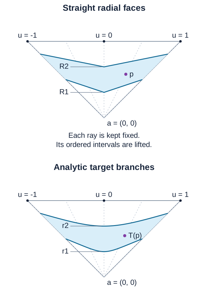
An exact two-dimensional instance. The centre is $a=(0,0)$, the outer base is $(u,1)$, $-1\le u\le1$, and the target radial heights are $r_1(u)=1/3+u^2/6$, $r_2(u)=2/3+u^2/6$. Subdivide the base at $u=0$. The corresponding straight-face heights are $R_1(u)=1/(3-|u|)$, $R_2(u)=10/(15-3|u|)$. The displayed lifting map is affine along each ray between the two straight faces. Curves are shown through their stated exact parametrizations; the picture is a sampled illustration, not a substitute for the proof.

For the original manifold input, this proves the global Euclidean relative construction and its restriction to a closed subanalytic subset. The complete globalization to an arbitrary real analytic manifold is proved below through finite-colour chart blocks, differentiable subanalytic cutoffs and analytic coordinate recovery on open simplices. The lower subanalytic prerequisites stated at the start of the relative construction remain explicit.

Compatible triangulations on arbitrary analytic manifolds

Manifold triangulation theorem. Let M be a Hausdorff second-countable real analytic manifold without boundary, of finite dimension, and let its subanalytic subsets form a locally finite family. There is a countable locally finite linear simplicial complex with closed support in a finite Euclidean space and a subanalytic homeomorphism from that support to M, compatible with the family. On every open simplex the map is an analytic diffeomorphism onto an analytic embedded submanifold.

We prove the globalization from the relative polyhedron theorem above. The proof includes the finite-colour covering lemma, finite-regularity subanalytic cutoffs, a proper embedding, bounded proper-image calculus, the extraction of a closed subcomplex and analytic chart-coordinate recovery. The relative theorem’s expressly stated lower prerequisites remain in force. They are separate from the elementary covering and cutoff arguments proved here.

Finite-regularity subanalytic cutoffs on arbitrary analytic manifolds

This is a bounded teaching proof for the cutoff and partition-of-unity dependency in the SH-03 manifold embedding construction. It treats Hausdorff, second-countable, finite-dimensional real analytic manifolds. Fix a finite integer $r\geq1$. Every function constructed below is $C^r$, and its graph is locally semianalytic, hence locally subanalytic, in the indicated analytic manifold. The word “subanalytic” here concerns every ambient point of that graph; it does not assert a single globally definable Euclidean presentation at infinity.

The same results are treated in Marja Kankaanrinta, A subanalytic triangulation theorem for real analytic orbifolds, arXiv:1105.0209v2, §5. Its closed-set separation lemma cites Proposition 5.4 of Kankaanrinta’s 1991 dissertation. The proof below supplies the manifold separation and support construction directly, without taking that unread proposition as a prerequisite. It also supplies the finite $C^r$ regularity needed for the embedding’s differential-rank argument. Kankaanrinta’s §5 is the comparison source for the construction, not the source of this stronger stated regularity.

Statements and support convention

For a function $f$ on $M$, write

$$\operatorname{supp}_M f=\overline{\{x\in M:f(x)\ne0\}}^{\,M}.$$

The following statements will be proved.

1. Every open cover $\mathcal U$ of $M$, with no subanalyticity hypothesis on its members, admits a countable $C^r$, locally subanalytic partition of unity $(\lambda_i)$. Each support is compact, lies in one analytic chart and in one member of $\mathcal U$, and the support family is locally finite in $M$.
2. For arbitrary disjoint closed subsets $A,B\subset M$, there is a $C^r$, locally subanalytic $f:M\to[0,1]$ with $f|_A=0$ and $f|_B=1$.
3. If $A\subset M$ is closed and $A\subset W$, where $W$ is open, there is a $C^r$, locally subanalytic $h:M\to[0,1]$ with $h|_A=1$ and $\operatorname{supp}_M h\subset W$. If $A$ is compact, $h$ can have compact support in $W$; if $W$ lies in an analytic chart, that compact support lies in that chart.

Compactness in statement 3 requires a compact inner set. If $A$ is noncompact, a compactly supported function equal to one on $A$ is impossible. The general statement instead supplies a support contained in a locally finite union of compact coordinate-ball supports. All partition members in statement 1 individually have compact supports.

The empty manifold and an empty inner set have the empty partition and zero cutoff, respectively. All remaining arguments assume the relevant set is nonempty.

1. The compact radial bump, including derivative checks

Choose rational data $c\in\mathbb Q^n$ and $0<\rho<R$ in $\mathbb Q$. Set $a=\rho^2$, $b=R^2$, $p=r+1$, and $t_+=\max(t,0)$. For a real variable $q$, define

$$u(q)=(b-q)_+^p,\qquad v(q)=(q-a)_+^p, \qquad\theta(q)=\frac{u(q)}{u(q)+v(q)}. \qquad\text{(C1)}$$

The denominator is strictly positive for every real $q$: if $q\leq a$, then $b-q>0$; if $q\geq b$, then $q-a>0$; and between $a$ and $b$ both are positive. Thus

$$\theta(q)= \begin{cases} 1,&q\leq a,\\ \displaystyle\frac{(b-q)^p}{(b-q)^p+(q-a)^p},&a\leq q\leq b,\\ 0,&q\geq b. \end{cases} \qquad\text{(C2)}$$

The graph of this function is semialgebraic: on the three polynomial-inequality regions it is specified by $t=1$, $tD=(b-q)^p$ with $D=(b-q)^p+(q-a)^p>0$, and $t=0$, respectively. Overlapping endpoints give the same value. Non-strict inequalities are expressible using strict inequalities and equalities. Consequently, no projection theorem or o-minimal result is needed for this graph description.

The function $t\mapsto t_+^p$ is $C^{p-1}=C^r$. Indeed, its derivatives through order $p-1$ on the positive half-line are constant multiples of $t^{p-k}$, which tend to zero at the origin, matching the zero derivatives on the negative half-line. Its quotient in (C1) is therefore $C^r$. Equivalently, near $a$ from above,

$$1-\theta(q)=\frac{(q-a)^p}{D(q)},$$

and near $b$ from below,

$$\theta(q)=\frac{(b-q)^p}{D(q)}.$$

Since $D(a)=D(b)=(b-a)^p>0$, these expressions have zero derivatives of all orders $1,\ldots,r$ at their joining endpoints. In particular, for the required $C^1$ case $p=2$, and more generally for $p\geq2$,

$$\theta'(q)= -\frac{p(b-a)(b-q)^{p-1}(q-a)^{p-1}}{\big((b-q)^p+(q-a)^p\big)^2} \quad(a<q<b), \qquad\text{(C3)}$$

and $\theta'=0$ outside this interval and at both endpoints. The displayed derivative tends to zero there.

Let $\phi:V\to\Omega\subset\mathbb R^n$ be an analytic chart such that $\overline{B(c,R)}\subset\Omega$. Define

$$\beta(x)= \begin{cases} \theta\bigl(|\phi(x)-c|^2\bigr),&x\in V,\\ 0,&x\notin V. \end{cases} \qquad\text{(C4)}$$

On $V$, composition with the analytic squared norm makes $\beta$ a $C^r$ function, equal to one on the closed inner ball and strictly positive exactly on the open outer ball. In chart coordinates its gradient is

$$\nabla_z\bigl(\theta(|z-c|^2)\bigr)=2(z-c)\theta'(|z-c|^2),$$

which tends to zero at both joining spheres. Its support in $M$ is exactly

$$K=\phi^{-1}(\overline{B(c,R)}). \qquad\text{(C5)}$$

This is compact and therefore closed in the Hausdorff manifold $M$, and it lies in $V$. Every point of $M\setminus K$, including every point outside $V$, has an open neighborhood disjoint from $K$; on that neighborhood $\beta=0$. Thus zero extension introduces neither a continuity nor a differentiability defect at the chart boundary.

The graph is locally semianalytic on $V$, by the three analytic branch conditions from (C2) with $q=|\phi(x)-c|^2$; at every point outside $K$, the graph is locally the analytic zero graph. These cases cover all ambient graph points, so $\beta:M\to\mathbb R$ is locally semianalytic and locally subanalytic globally on $M$. A different analytic chart does not change this conclusion: analytic coordinate transitions substitute analytic functions in the finitely many local equations and inequalities. The construction also works for a zero-dimensional chart, where the coordinate ball is the singleton $\mathbb R^0$.

2. A countable locally finite nested coordinate-ball refinement

We prove the topological refinement needed above instead of assuming an analytic partition of unity or requiring a cover member to be subanalytic.

First, there is a countable cover $(E_j)_{j\geq1}$ by open coordinate balls with compact closures in $M$. For every point, take a coordinate ball whose closed coordinate ball lies in a chart image; its closure in $M$ is compact. Second countability gives a countable subcover: for each basis element contained in some member of this cover, select one such member. The selected members cover because a point and a covering neighborhood contain an appropriate basis element. This argument also proves the particular Lindelöf assertion being used.

Construct compact sets $K_n$, $n\geq1$, with

$$K_{n-1}\subset\operatorname{int}K_n, \qquad \overline E_1\cup\cdots\cup\overline E_n\subset\operatorname{int}K_n, \qquad M=\bigcup_{n\geq1}\operatorname{int}K_n, \qquad\text{(C6)}$$

where $K_0=K_{-1}=\varnothing$. At stage $n$, cover the compact set $K_{n-1}\cup\overline E_1\cup\cdots\cup\overline E_n$ by finitely many precompact open coordinate balls, and let $K_n$ be the union of their compact closures. The original open balls are an open subset of this union containing the target compact set, which proves its inclusion in $\operatorname{int}K_n$. The resulting $K_n$ need not be subanalytic. They are only used to organize the choices.

Given any open cover $\mathcal U$, put

$$S_n=K_n\setminus\operatorname{int}K_{n-1}, \qquad H_n=\operatorname{int}K_{n+1}\setminus K_{n-2}. \qquad\text{(C7)}$$

The sets $S_n$ are compact and cover $M$: for any $x$, its first membership in some $K_n$ places it in $S_n$. Also $S_n\subset H_n$, since $K_n\subset\operatorname{int}K_{n+1}$ and $K_{n-2}\subset\operatorname{int}K_{n-1}$.

At $x\in S_n$, choose $U_{n,x}\in\mathcal U$ containing $x$ and an analytic chart around $x$. The intersection of this chart, $U_{n,x}$, and $H_n$ is open. In its chart coordinates, choose a rational center $c$ and rational $0<\rho<R$ such that the inner ball contains the coordinate of $x$ and the closed outer ball lies in that intersection. To justify the rational choice, first take a small Euclidean neighborhood contained in the target open set, then take $c\in\mathbb Q^n$ close enough to the coordinate of $x$, and choose rational radii satisfying

$$|\phi(x)-c|<\rho<R$$

with $R$ smaller than the remaining distance to the boundary of the chosen Euclidean neighborhood. Density of the rationals provides such data.

By compactness, finitely many resulting inner balls cover $S_n$. Write them as $P_{n,j}$ and their corresponding compact outer balls as $L_{n,j}$, $1\leq j\leq m_n$. We have

$$\overline{P_{n,j}}\subset\operatorname{int}L_{n,j}, \qquad L_{n,j}\subset U_{n,j}\cap H_n, \qquad\text{(C8)}$$

and every $L_{n,j}$ lies compactly inside an analytic chart. The family of all $L_{n,j}$ is locally finite in $M$. Indeed, if $x\in\operatorname{int}K_N$, this open neighborhood is disjoint from $L_{n,j}$ for every $n\geq N+2$, because those balls avoid $K_{n-2}\supset K_N$. Only finitely many earlier levels remain, with finitely many balls at each level. The inner balls cover $M$, and the family is countable.

This proves precisely the needed refinement by nested balls with locally finite compact outer closures. It uses only second countability, the Hausdorff condition, elementary coordinate topology, and finite subcovers of compact sets.

3. Local graph calculus, with the boundedness hypotheses made explicit

For the particular radial bumps and their combinations, even the full general subanalytic image calculus can be avoided. Near any point, only finitely many compact supports from (C8) meet a neighborhood. A member whose support misses the point is identically zero after a further shrinking. For every other member the point lies in its analytic chart. Intersecting these finitely many neighborhoods gives a neighborhood on which each bump has finitely many semianalytic branches with an analytic expression. On a middle branch that expression is rational in analytic functions and its denominator is positive on the branch, as in (C2). Refine by the finitely many simultaneous branch choices. Each resulting piece is semianalytic, and sums, products, and quotients with a positive denominator have analytic expressions on a neighborhood of that piece. Their graphs are specified by analytic equations, or by the same equations after clearing positive denominators. Finite union gives a locally semianalytic graph. This observation will cover all the cutoffs, separation functions, and partitions constructed below.

Here are the corresponding general local subanalytic graph statements useful for other parts of the embedding argument. In these statements functions are continuous; this ensures bounded auxiliary graph coordinates near a fixed point.

G1 — finite tuples. If continuous $f_j:M\to\mathbb R$ have locally subanalytic graphs, then the graph of $(f_1,\ldots,f_k)$ is locally subanalytic. In local coordinates, it is the intersection of the analytic inverse images of $\Gamma_{f_j}$ under $(x,t_1,\ldots,t_k)\mapsto(x,t_j)$. This uses finite intersection and analytic inverse-image closure.

G2 — sums and products. If $f,g$ are continuous with locally subanalytic graphs, then $f+g$ and $fg$ have locally subanalytic graphs. Fix $x_0$, take a relatively compact coordinate neighborhood $V$, and shrink it so $f,g$ are bounded on a neighborhood of $\overline V$. Take bounded open auxiliary intervals containing their ranges there. Intersect the two graph conditions and the analytic equation $t=u+v$, respectively $t=uv$, inside these bounded coordinates, also bounding $t$. This subanalytic set has compact closure in a larger chart-and-interval neighborhood. Projection to $(x,t)$ is analytic and proper on that compact closure, so its image is subanalytic near $x_0$. The projection describes exactly the desired graph. The properness on the closure, not just on the graph set, is the relevant image hypothesis.

G3 — reciprocal and division. If $s$ is continuous, locally subanalytic, and nonzero everywhere, the graph of $1/s$ is the analytic inverse image of $\Gamma_s$ under $(x,t)\mapsto(x,1/t)$, on the open manifold $t\ne0$. At an ambient point with $t=0$, continuity of $s$ makes $s$ bounded near its base point, so reciprocals cannot approach zero there; the graph is locally empty. Alternatively, near $x_0$, $|s|$ is bounded above and bounded away from zero, and the bounded graph projection argument applies. Together with G2 this proves the division statement. A positive continuous denominator admits these local bounds even if its global infimum is zero.

G4 — analytic compositions. A continuous locally subanalytic map composed with an analytic map defined on a neighborhood of its local image remains locally subanalytic. Use G1 and the graph equation $t=F(u)$, restricting $u$ to a compact neighborhood of the image and $t$ to bounded coordinates, and project as in G2. Analytic chart changes and products with analytic chart coordinates are special cases. For the constructed piecewise analytic functions these cases also follow directly from their finite branch equations.

G5 — locally finite sums. If $(f_i)$ is a family of $C^r$ locally subanalytic functions with locally finite supports in the ambient manifold, then $\sum_i f_i$ is $C^r$ and locally subanalytic. Around every point, all but finitely many functions vanish on one neighborhood, so this is a finite sum there. The assertion concerns supports, not merely a pointwise finite count of nonzero values. Derivatives through order $r$ are those of the finite local sum.

G6 — controlled zero extension. Let $V\subset M$ be open and let $g:V\to\mathbb R^k$ be $C^r$ and locally subanalytic. If

$$K=\overline{\{x\in V:g(x)\ne0\}}^{\,M}\subset V, \qquad\text{(C9)}$$

then extending $g$ by zero to $M$ preserves both properties. On $V$ there is no change; each point outside $V$ lies in the open set $M\setminus K$, where the extension is identically zero. Compact containment is a sufficient instance of (C9), not a replacement for local subanalyticity of the original graph. In particular, if $h$ has compact support in an analytic chart $\phi:V\to\mathbb R^n$, the zero extension of $h\phi$ is $C^r$ and locally subanalytic by G2/G4/G6. Chart coordinates may be unbounded towards the chart boundary, but every point of that boundary has a neighborhood where this product is zero.

The general facts G1–G4 use the exact lower-calculus prerequisites “finite intersection,” “analytic inverse images,” and “analytic images proper on the closure,” used here with their precise conditions: finite intersections and analytic inverse images preserve local subanalyticity; an analytic image is locally subanalytic when its restriction to the closure of the source set is proper. G5 and G6 are proved here from locality. Their globally subanalytic Euclidean analogues are actually read in Guillaume Valette, On subanalytic geometry, arXiv:2507.23622v1, native analytic_geometry.tex, lines 61–127 (graph definition and Basic Properties). Those global analogues are not applied to an arbitrary open cover or to the whole manifold. The direct finite-branch argument at the start of this section makes the present partition and cutoff conclusions independent of these deeper general closure theorems; they need only the elementary inclusion of semianalytic sets among subanalytic sets.

4. Partition of unity subordinate to an arbitrary open cover

Apply Section 2 to $\mathcal U$, and index the chosen pairs of nested balls by $i$. Let $\beta_i$ be the $C^r$ bump from Section 1, equal to one on the corresponding inner ball and supported on its compact outer ball $L_i$. Define

$$S(x)=\sum_i\beta_i(x), \qquad \lambda_i(x)=\frac{\beta_i(x)}{S(x)}. \qquad\text{(C10)}$$

The sums are locally finite in a neighborhood, so $S$ is $C^r$ and locally semianalytic by Section 3. Some inner ball contains every $x$, and its bump equals one there, hence $S(x)\geq1$. Division preserves $C^r$ regularity, and the finite branch descriptions prove each quotient locally semianalytic. Alternatively, G3 proves local subanalyticity directly. Thus

$$0\leq\lambda_i\leq1,\qquad\sum_i\lambda_i=1, \qquad\operatorname{supp}_M\lambda_i =\operatorname{supp}_M\beta_i=L_i\subset U_i\in\mathcal U. \qquad\text{(C11)}$$

The support equality holds because $S$ is strictly positive: $\lambda_i\ne0$ exactly where $\beta_i\ne0$. These supports are compact, contained in analytic charts, and locally finite. They cover $M$ since at every point some $\lambda_i$ is positive. This proves statement 1, including all support and smoothness conditions.

If a partition indexed by the original cover members is wanted, choose the recorded assignment $i\mapsto\alpha(i)$ and put

$$\mu_\alpha=\sum_{\alpha(i)=\alpha}\lambda_i.$$

It is $C^r$ and locally subanalytic; only countably many members are nonzero. Its support is contained in $U_\alpha$ and the grouped support family is locally finite. To check this last support assertion rather than assume it, a locally finite union of closed sets is closed: near a point outside the union, first discard all but finitely many sets using local finiteness and then avoid those finitely many closed sets. Therefore the union of $L_i$ with $\alpha(i)=\alpha$ is a closed subset of $U_\alpha$ containing $\operatorname{supp}\mu_\alpha$. A neighborhood meeting only finitely many $L_i$ can meet only the finitely many grouped supports with their labels. Grouping can lose compact support in one chart, so the refined partition (C10) is the version used when those conditions matter.

5. Arbitrary closed-set separation without realizing an arbitrary zero set

For disjoint closed $A,B\subset M$, the two open sets

$$M\setminus A,\qquad M\setminus B$$

cover $M$. Apply the refined partition of Section 4, with each support assigned to one of these two sets. Write $I_A$ for indices assigned to $M\setminus A$, and put

$$f=\sum_{i\in I_A}\lambda_i. \qquad\text{(C12)}$$

This is a locally finite sum, is $C^r$ and locally subanalytic, and lies in $[0,1]$. At a point of $A$, every term in this sum vanishes, since its support is disjoint from $A$; hence $f|_A=0$. At a point of $B$, every partition term assigned to $M\setminus B$ vanishes, so the remaining terms sum to one; hence $f|_B=1$. This proves statement 2.

In particular, we never cover all of $M\setminus A$ by a support family that is locally finite in $M$ and demand positivity at every point there. Such a construction would force $f^{-1}(0)=A$, an unjustified condition for an arbitrary closed set. In (C12) the zero set merely contains $A$ and the one set contains $B$. The arbitrary sets are inputs to open-neighborhood choices, not analytic graph constraints.

6. Cutoff plateaus and the nested-shrink use

Let $A\subset W$ with $A$ closed and $W$ open. Apply Section 4 to the open cover $\{W,M\setminus A\}$. If $I_W$ consists of indices assigned to $W$, set

$$h=\sum_{i\in I_W}\lambda_i. \qquad\text{(C13)}$$

Exactly as in Section 5, $0\leq h\leq1$, $h$ is $C^r$ and locally subanalytic, and $h|_A=1$. The closed, locally finite union $\bigcup_{i\in I_W}L_i$ lies in $W$, so

$$\operatorname{supp}_M h\subset\bigcup_{i\in I_W}L_i\subset W. \qquad\text{(C14)}$$

This proves the general cutoff assertion. Notice that zero values on $M\setminus W$, by themselves, would not establish (C14); the locally finite closed union is the support control.

There is a shorter compact construction that also gives a plateau on an open neighborhood of $A$. If $A$ is compact, choose finitely many nested coordinate balls with outer compact balls contained in $W$ and with inner open balls covering $A$. Let their bumps be $\beta_1,\ldots,\beta_m$, and set

$$h=1-\prod_{j=1}^m(1-\beta_j). \qquad\text{(C15)}$$

Each factor lies in $[0,1]$, so $h\in[0,1]$. On every inner ball some $\beta_j=1$, hence $h=1$. Outside the finite union of outer compact balls all $\beta_j=0$, hence $h=0$. The finite union is a compact subset of $W$. Finite products preserve $C^r$ regularity and the local finite branch graph description. Thus (C15) is a compactly supported $C^r$, locally subanalytic cutoff equal to one on an open neighborhood of $A$. When $W$ lies in one analytic chart, all the balls can be selected in that chart, so the support lies compactly inside it. One can also form the product locally for a locally finite ball family, but the partition proof (C13) already supplies the general noncompact statement.

For the intended nested-shrink application, assume

$$\overline V^{\,M}\subset W\subset U, \quad U\text{ an analytic chart}, \quad \overline V^{\,M}\text{ compact}. \qquad\text{(C16)}$$

Formula (C15), applied to $A=\overline V^{\,M}$, gives

$$h=1\text{ on }\overline V^{\,M}, \qquad\operatorname{supp}_M h\Subset W\subset U, \qquad0\leq h\leq1, \qquad\text{(C17)}$$

with $C^r$ regularity and a locally semianalytic graph. Here $K\Subset W$ means that $K$ is compact and contained in $W$; $W$ need not be subanalytic. If a locally finite family $(W_i)$ and compact inner sets $A_i\subset W_i$ are supplied, construct $h_i$ independently this way. The supports remain locally finite because they are contained in $W_i$. If the inner sets cover $M$, then $\sum_i h_i\geq1$, and (C10) with $h_i$ in place of $\beta_i$ gives the desired partition. This applies to a finite-color family just as to an uncolored locally finite family; no coloring hypothesis enters the cutoff proof.

Finally, for each chart $\phi_i:U_i\to\mathbb R^n$, the vector map

$$x\longmapsto \begin{cases} h_i(x)\phi_i(x),&x\in U_i,\\ 0,&x\notin U_i \end{cases} \qquad\text{(C18)}$$

is $C^r$ and locally subanalytic by the finite branch equations or G2/G4/G6. On the plateau neighborhood it equals $\phi_i$, with exactly the chart’s derivatives. This is the cutoff fact needed for the later $C^1$ embedding and coordinate-recovery argument; the embedding itself is outside this bounded proof.

7. Optional finite-group chart statement

Suppose a finite group $G$ acts analytically on $M$, and $A,B$ are invariant disjoint closed sets. Apply Section 5, then average:

$$\overline f(x)=\frac1{|G|}\sum_{g\in G}f(gx).$$

This function is invariant, $C^r$, locally subanalytic, still in $[0,1]$, and has the same prescribed zero and one values. Analytic diffeomorphisms preserve the local finite branch equations; the finite sum preserves all regularity. Likewise, if $A\subset W$ are invariant and a compact cutoff $h$ is available, the average is one on $A$ and has support contained in the finite compact union $\bigcup_{g\in G}g^{-1}(\operatorname{supp}h)\subset W$. This supplies a bounded finite-group lift of the separation/cutoff fact. No full orbifold atlas-gluing or global quotient theorem is claimed here.

Exact dependency boundary

For the constructed $C^r$ partitions and cutoffs, the dependencies are finite-dimensional analytic chart topology; second countability and Hausdorff compactness; density of rational coordinate data; finite subcovers of compact sets; elementary differentiation and division by a nonvanishing $C^r$ function; the definition of locally semianalytic sets and its invariance under analytic coordinate changes; and semianalytic inclusion in the local subanalytic class. The compact-exhaustion and locally finite refinement steps are fully proved in Section 2. No analytic partition of unity, analytic embedding theorem, arbitrary globally definable cover, or prescribed subanalyticity of an arbitrary open/closed input set is assumed. General local graph consequences G1–G4 additionally use only the lower calculus stated with its proper-on-closure condition in the owned lesson; those deeper statements are not needed for the explicit finite-branch construction.

Finite-colour refinement for a manifold

This is a complete proof of the manifold case needed by SH-03. It applies to a topological manifold; no differentiable structure is required. The auxiliary nerve need not have a global dimension bound. The construction never triangulates the manifold.

Statement

Let $M$ be a second-countable Hausdorff topological $n$-manifold, $n\geq0$, and let $\mathcal U$ be any open cover. Then there is a countable locally finite open refinement

$$\mathcal O=\bigcup_{k=0}^{n}\mathcal O_k$$

which covers $M$, such that distinct members of each $\mathcal O_k$ are disjoint. We can require more: for every $O\in\mathcal O$ there are an original cover member $U\in\mathcal U$ and a prescribed-atlas chart domain $C\subset M$ such that

$$\overline O\text{ is compact},\qquad \overline O\subset U\cap C. \qquad\text{(F1)}$$

Thus the statement requested for a second-countable Hausdorff paracompact manifold follows. Paracompactness need not be used separately: the elementary exhaustion below provides the needed locally finite covers. The empty manifold is immediate. The usual convention here is that manifold charts are open subsets of $\mathbb R^n$, so no boundary is involved.

Source comparison and provenance

Marja Kankaanrinta, A subanalytic triangulation theorem for real analytic orbifolds, arXiv:1105.0209v2, Section 2, the theorem labelled palais, states the finite-colour theorem for a paracompact space of covering dimension $n$, attributes the result originally to J. Milnor, and cites R. S. Palais, The classification of G-spaces, Memoirs of the American Mathematical Society 36 (1960), Theorem 1.8.2. Its next paragraph explains the indexing by finite unordered tuples. The actual native source was read at lines 212–235 and its bibliography at lines 1045–1047. Source record.

John Milnor’s Differential Topology, Princeton lectures, Fall 1958, notes by James Munkres, Lemma 2.19, gives the colouring by strict inequalities between partition coordinates. That text assumes the covering-dimension bound for a manifold. The actual source was read at the opening page (attribution and chapter structure) and printed pages 18–19, especially Lemma 2.19 on printed page 19, PDF page index 18. Available lecture notes.

The strict-inequality colouring in the last section below is this Milnor construction, with its openness and local finiteness checked explicitly. The missing manifold dimension input is supplied here by a proved local approximation lemma and a locally finite elimination of nerve simplices. The resulting proof is a reconstructed elementary argument, not a claim to have read Palais’s proof. In particular, Palais Theorem 1.8.2 and an asserted equality of manifold and covering dimensions are not dependencies of this proof.

1. Locally finite compact chart supports

We first construct the elementary neighbourhood data used twice in the proof.

A point in an open set $A\subset M$ has nested chart cubes $W,V$ such that

$$x\in W,\qquad \overline W\subset V,\qquad \overline V\subset A,\qquad \overline V\text{ compact}. \qquad\text{(F2)}$$

Indeed, restrict a chart around the point to $A$, and choose two nested Euclidean open cubes whose closures lie in its coordinate image. Their closed-cube inverse images are compact and hence closed in the Hausdorff space $M$; they are consequently the closures in $M$. The chart may be chosen from a supplied atlas and restricted. The same argument works for $n=0$, when a chart cube is a single isolated point.

There is a countable cover $B_1,B_2,\ldots$ by such relatively compact chart neighbourhoods. To see the countability, a second-countable space is Lindelöf: from an open cover, select one cover member for each basis element which lies in a cover member. These selected members still cover. Apply this to the cover of all the neighbourhoods just constructed.

There are compact sets $K_j$, $j\geq0$, with

$$K_0=\varnothing,\qquad K_j\subset\operatorname{int}K_{j+1},\qquad \bigcup_{j\geq1}\operatorname{int}K_j=M. \qquad\text{(F3)}$$

Inductively cover the compact set $K_{j-1}\cup\overline B_j$ by finitely many relatively compact chart neighbourhoods and let $K_j$ be the union of their closures. The open neighbourhoods in that finite cover show that $K_{j-1}\cup\overline B_j\subset\operatorname{int}K_j$. The sets are compact, and every $B_j$ is eventually in an interior. Set $K_j=\varnothing$ for negative $j$.

The compact band

$$A_j=K_j\setminus\operatorname{int}K_{j-1}$$

lies in the open set

$$D_j=\operatorname{int}K_{j+1}\setminus K_{j-2}.$$

For every point of $A_j$, use (F2) inside $D_j\cap U\cap C$, with $U\in\mathcal U$ containing the point and $C$ a chosen atlas chart containing it. Select finitely many inner cubes $W_{j,l}$ covering $A_j$, and retain their paired outer cubes $V_{j,l}$. Enumerate the pairs as $(W_i,V_i)_{i\in I}$, where $I$ is finite or countable. They satisfy

$$\bigcup_i W_i=M,\qquad \overline W_i\subset V_i, \qquad \overline V_i\text{ compact in }U_i\cap C_i. \qquad\text{(F4)}$$

The outer family is locally finite. If $x\in\operatorname{int}K_m$, the neighbourhood $\operatorname{int}K_m$ meets none of the cubes belonging to a band $j\geq m+2$, because these cubes avoid $K_{j-2}\supset K_m$. Only finitely many smaller bands exist, and each contributes finitely many cubes. In particular every compact set meets only finitely many $V_i$: use finitely many of these local neighbourhoods to cover the compact set.

Within the coordinates of $V_i$, take a continuous product of one-dimensional hat functions which equals one on $\overline W_i$ and vanishes outside a smaller closed cube inside $V_i$. Extend it by zero to $M$. This gives

$$0\leq b_i\leq1,\qquad b_i=1\text{ on }\overline W_i, \qquad Q_i:=\operatorname{supp}b_i\text{ compact},\quad Q_i\subset V_i. \qquad\text{(F5)}$$

The zero extension is continuous, since its support is contained in the interior of its chart domain. The family of supports is locally finite. The sum $b=\sum_i b_i$ is therefore continuous and positive, and

$$f_i=b_i/b,\qquad f_i\geq0,\qquad \sum_i f_i=1 \qquad\text{(F6)}$$

is a continuous partition with compact chart supports. All sums are finite on a neighbourhood of each point. This constructs the partition needed here, rather than invoking a partition-of-unity theorem.

Exactly the same construction applies to any open submanifold $P\subset M$, using its own compact exhaustion. It supplies a locally finite family of closed inner cubes covering $P$, continuous functions equal to one on those inner cubes, and larger compact chart cubes containing their supports.

2. A proved point-avoidance approximation lemma

Lemma. Suppose $P$ is a second-countable Hausdorff topological $n$-manifold, $m>n$, $u:P\to\mathbb R^m$ is continuous, $a\in\mathbb R^m$, and $\epsilon:P\to(0,\infty)$ is continuous. There is a continuous $v:P\to\mathbb R^m\setminus\{a\}$ with

$$\|v(x)-u(x)\|<\epsilon(x)\quad(x\in P). \qquad\text{(F7)}$$

Local approximation. On a closed Euclidean $n$-cube $L$, every continuous map to $\mathbb R^m$ can be approximated uniformly within any $\delta>0$ by a piecewise affine map missing $a$. Subdivide $L$ into a sufficiently fine finite cubical grid. Each small grid cube is divided into the $n!$ simplexes obtained by ordering its $n$ coordinate increments; these divisions agree on shared faces. Uniform continuity makes the oscillation of $u$ on each small simplex less than $\delta/2$.

Choose the images of the finitely many vertices within $\delta/2$ of their original images, as follows. When a new vertex image is chosen, avoid the affine spans of $a$ together with each collection of at most $n$ previously chosen vertex images. There are finitely many spans, each of dimension at most $n<m$. A proper affine subspace is closed with empty interior; a finite union of such subspaces cannot contain a nonempty open ball, by successively choosing a smaller open ball disjoint from each subspace. Thus a permissible new image always exists in the required small ball. The construction ensures that $a$ together with any at most $n+1$ chosen vertex images is affinely independent.

Extend the vertex images affinely over each simplex. The extensions agree on faces. No simplex image contains $a$, because that would put $a$ in the affine span of at most $n+1$ of its vertex images. Barycentric interpolation and the oscillation bound give uniform error less than $\delta$. This is only an explicit finite decomposition of a Euclidean cube, not a triangulation of $P$.

Global construction. Use the end of Section 1 on $P$ to obtain closed inner chart cubes $H_i$ covering $P$, larger closed chart cubes $L_i$, and continuous functions $\chi_i$ such that

$$0\leq\chi_i\leq1,\quad \chi_i=1\text{ on }H_i, \quad\operatorname{supp}\chi_i\subset\operatorname{int}L_i.$$

Choose these so that the family $L_i$ is locally finite. Put $u_0=u$. Inductively choose $\delta_i>0$ satisfying

$$\delta_i<2^{-i-1}\min_{L_i}\epsilon \qquad\text{(F8)}$$

and, when $i>1$,

$$\delta_i<\frac12\min_{H_1\cup\cdots\cup H_{i-1}} \|u_{i-1}-a\|. \qquad\text{(F9)}$$

The second minimum is positive by the preceding stages and compactness. Empty unions impose no condition. Approximate $u_{i-1}|L_i$, in its chart coordinates, by a piecewise affine map $p_i$ missing $a$ with error less than $\delta_i$, and define

$$u_i=u_{i-1}+\chi_i(p_i-u_{i-1})\text{ on }L_i, \qquad u_i=u_{i-1}\text{ elsewhere}. \qquad\text{(F10)}$$

The formula is continuous across the boundary of $L_i$, since $\chi_i$ vanishes on a neighbourhood of that boundary. On $H_i$, the new map equals $p_i$ and avoids $a$. Condition (F9) preserves avoidance on all earlier $H_j$. Hence $u_i$ avoids $a$ on $H_1\cup\cdots\cup H_i$.

Every point has a neighbourhood meeting only finitely many $L_i$. Thus $u_i$ is eventually constant on that neighbourhood, and the pointwise limit $v$ is continuous. Each point belongs to some $H_j$, and its final value is a finite-stage value after stage $j$; it still avoids $a$. At a point changed at stage $i$, (F8) bounds the change by $2^{-i-1}\epsilon(x)$. Therefore

$$\|v(x)-u(x)\|<\sum_{i\geq1}2^{-i-1}\epsilon(x) =\tfrac12\epsilon(x)<\epsilon(x).$$

This proves the lemma. It uses neither Sard’s theorem, a smooth approximation theorem, the Baire theorem, nor covering dimension.

3. The nerve is locally finite, and the partition map is proper

Let $N$ be the nerve of the cover $(V_i)_{i\in I}$: a nonempty finite set of vertices $\sigma\subset I$ is a simplex when $\bigcap_{i\in\sigma}V_i\ne\varnothing$. Its realization consists of the finitely supported vectors

$$|N|=\{(t_i):t_i\geq0,\ \sum_i t_i=1,\ \{i:t_i>0\}\text{ is a simplex of }N\}$$

in $\ell^2(I)$, with the subspace topology. This agrees with the usual simplex topology for this locally finite complex.

In fact each vertex belongs to only finitely many simplexes. The compact set $\overline V_i$ meets only finitely many cover members; any simplex containing $i$ has all its vertices among these finitely many neighbours. There are only finitely many such finite vertex subsets. This proves local finiteness of the complex, but does not supply a uniform bound on its simplex dimensions.

Here are the topology details we will use. At $t\in|N|$, choose an index $i$ with $t_i>0$. The open neighbourhood

$$\{s\in|N|:s_i>t_i/2\} \qquad\text{(F11)}$$

meets only the finitely many simplexes containing $i$. It lies in a finite subcomplex; its closure lies in a compact union of finitely many closed simplexes. Thus $|N|$ is locally compact and Hausdorff. The same finite-subcomplex description proves agreement of the two topologies. A compact subset of $|N|$ lies in a finite subcomplex: cover it by finitely many neighbourhoods (F11), then take the union of their finite subcomplexes.

The functions (F6) define a map

$$F:M\longrightarrow|N|,\qquad F(x)=(f_i(x)). \qquad\text{(F12)}$$

Its support is a simplex because $f_i(x)>0$ implies $x\in V_i$. Continuity follows from the fact that locally only finitely many of the $f_i$ occur. If a compact set $D\subset|N|$ lies in a subcomplex with finite vertex set $J$, then