Subanalytic sets and limiting tangent directions
At a smooth point, a one-form can be tested on the tangent space. At a singular point, an approach to the set may have zero first derivative, and the first useful displacement may occur several orders later. Subanalytic geometry lets us replace such a limiting approach by an analytic curve and retain its first nonzero term. This gives a precise meaning to a one-form vanishing on a singular set, and explains why that condition survives analytic maps.
We work with finite-dimensional real analytic manifolds, Hausdorff and countable at infinity. All maps called analytic are real analytic. No coefficient ring or sheaf boundedness condition enters this geometric lesson. Later, these results will control cotangent supports of constructible sheaves.
The proof has three routes. Analytic curves turn limiting displacements into leading Taylor coefficients; proper uniformization lets tangent vectors detect a one-form; ordered radial graphs produce compatible triangulations. These routes share subanalytic set calculus but use different additional inputs. The signed normal-deformation criterion comes from the normal-geometry course.
Original exposition by GPT-6.1 Sol (OpenAI), Ultra, September–October 2026; revised by GPT-6 Astra (OpenAI), Ultra, October 2026. Original programme expression is public domain (CC0). Human results retain their named credit, and the linked Valette adaptations retain CC BY 4.0.
A local class with controlled boundaries
A subset is subanalytic if, near every point of the ambient manifold, it has a presentation
where the are compact real analytic manifolds and the are analytic. Both the neighborhood and the finite presentation can depend on the ambient point. In particular, behavior at a boundary point outside still matters.
An equivalent description uses local projections of relatively compact semianalytic sets. A semianalytic set is locally a finite Boolean combination of analytic equalities and strict inequalities. This description makes analytic rank conditions, specified by minors of a differential, available inside the subanalytic calculus. The compact-image construction below proves the equivalence with (1), including the converse for arbitrary subsets by a terminating sequence of frontier differences.
The following six statements fix the scope of the lesson. The compact-image construction proves the set and map calculus in item 1. The dimension-controlled proper uniformization proves item 4 on arbitrary noncompact manifolds as well, with a source of the same dimension as the set. The analytic-descent and squared-distance argument proves every fixed-dimensional intrinsic regular-locus statement in item 2. Curve selection is connected below to its explicit local-chart and Puiseux providers, and compatible triangulation is constructed first on a relative polyhedron and then on an arbitrary manifold. The analytic-function resolution in item 5 is proved below by constructing the local invariant, closed canonical centres and finite local towers, and then comparing and gluing those towers. The proof retains the entire function and its multiplicities.
- Set operations and analytic maps. Closure, interior, finite union, intersection and difference preserve subanalyticity. Connected components are subanalytic and form a locally finite family in the ambient manifold. Analytic inverse images are subanalytic. If is analytic, is subanalytic, and is proper, then is subanalytic. The bar in this properness hypothesis is essential.
- Regular points. A point of is regular when is a closed analytic submanifold of some ambient neighborhood . Write for these points. The regular locus and its complement in are subanalytic; . For each fixed dimension , the dimension- part of the regular locus is subanalytic. We set , with the usual empty-set convention. The intrinsic regular-locus proof below establishes these statements using analytic descent and squared distance, with the Bierstone–Milman source credited there.
- Curve selection. If , there is an analytic curve with and for every . Its first derivative may vanish. The two-sided parameter is compatible with a one-sided set: squaring an initially positive parameter produces it.
- Uniformization. A closed subanalytic set is the image of an analytic manifold under a proper analytic map . For nonempty , the source can have pure dimension ; if is compact, the source can be compact.
- Resolution of an analytic function. Suppose is analytic and is not identically zero on any connected component. Put . There is a proper analytic , an isomorphism over , such that near each point of , in analytic coordinates, Exponents equal to zero are allowed.
- Compatible triangulation. Every locally finite subanalytic partition of admits a locally finite simplicial triangulation whose open simplices have subanalytic analytic-submanifold images, each lying in one member of the partition. The triangulating map is a homeomorphism. Its global analyticity is not asserted. This is the bridge to Constructible sheaves on a triangulation.
Local finiteness extends the finite set-operation statements to a locally finite union: near any ambient point, only finitely many members occur. It does not authorize arbitrary unions. Likewise, analytic maps need not preserve subanalyticity of their images without the stated control at infinity.
Analytic coordinates and uniqueness with parameters
The coordinate arguments here require analytic charts and inverses. Their starting point is the proved holomorphic inverse and implicit function theorem, Lemma 2.2. The proof uses a uniformly contracting iteration on a small complex ball; its iterates are holomorphic, and Cauchy’s formula makes their locally uniform limit holomorphic. We record the passage to real analytic maps, including parameters, and the differential-equation fact needed by the finite-jet construction.
Real analytic inverse, implicit and constant-rank coordinates
A real analytic power series, on a sufficiently small neighborhood of its centre, extends to a holomorphic power series on a complex polydisc. Indeed, absolute convergence on a smaller real box bounds the series with the absolute values of its coefficients; the same bound applies to complex arguments of those moduli. Its coefficients are real, so this extension commutes with conjugation.
Analytic inverse theorem with parameters. Let be real analytic near , with , , and assume is invertible. There is a unique local real analytic map solving
Proof. Complexify near the specified point. The block map has invertible derivative there. Apply the holomorphic inverse theorem. Its inverse preserves the last coordinate because the map itself does. After taking conjugation-invariant neighborhoods, uniqueness implies that the inverse commutes with conjugation: conjugating the unique preimage of a real target gives that same preimage. Restriction to real points therefore gives a real analytic inverse. The convergent complex power series of its components restrict to the required real power series. Both identities follow from the two inverse identities.
Consequently, if is real analytic, , and is invertible, the map has a real analytic inverse. Its middle target coordinate equal to zero gives a unique real analytic solution . More generally, independent defining differentials can be completed by linear coordinate functions to an invertible square Jacobian. This gives analytic submersion coordinates, analytic local sections, and analytic level submanifolds, with tangent space the kernel of the differential.
Analytic constant-rank theorem with parameters. Suppose is real analytic and throughout a neighborhood of . There are real analytic source and target coordinate changes, both preserving , in which the map becomes The hypothesis is constant rank in the variables on a neighborhood, not merely a rank calculation at the central point.
Proof. For , reorder source and target coordinates so an -by- minor is invertible at the specified point. The map has invertible derivative and is an analytic coordinate change by (LAF1). On a smaller product box, the transformed map has the form At each fixed parameter its derivative in is Its rank equals , by subtracting times the upper block rows from the lower block rows. Condition (LAF3) forces . Integrating each derivative along coordinate segments inside the product box shows . The analytic target change has the explicit analytic inverse which adds , and gives (LAF4). For , the same segment argument makes independent of , and subtraction of this parameter-dependent value finishes the proof.
Taking no parameters gives the analytic constant-rank theorem on manifolds by using charts. It proves, in particular, that a local constant-rank fibre is an analytic manifold with tangent space . A map with injective differential is locally an analytic embedding. If it is also a homeomorphism onto its image, these local descriptions give an embedded analytic submanifold globally on that image.
Analytic differential equations
For the finite-jet argument, uniqueness is already supplied by Local tools for bundles and transport, Theorem 2.1. That theorem proves uniqueness among differentiable solutions and smooth dependence on all initial data. Analytic dependence is a stronger assertion; the following direct construction establishes it when the vector field is analytic.
Analytic parameter theorem. For a real analytic finite system the local solution is real analytic jointly in . It is the unique differentiable real solution with those data on any common connected interval where the solutions are defined.
Proof. Translate a fixed datum to the origin and extend holomorphically to a complex product neighborhood. Use the maximum norm on coordinates and its induced operator norm for matrices. Choose positive whose closed product polydisc is inside that neighborhood, and bounds for and there. The spatial segment formula gives inside the convex spatial polydisc. Choose so Restrict , , and . If a bound is zero, its corresponding inequality imposes no restriction.
Starting with , define, for , The integral is over the straight complex segment. Every iterate has spatial norm at most : its norm is at most whenever the preceding iterate has that bound. Its time argument stays inside .
Every iterate is jointly holomorphic. To verify the integration step, write the integral as . On each smaller closed parameter polydisc the integrand is uniformly continuous in ; the Riemann sums are holomorphic and converge uniformly. The holomorphic convergence theorem, Theorem 3.1, makes the integral holomorphic.
Take suprema over the entire smaller data product and . The spatial estimate gives The geometric tail bound proves uniform convergence to a jointly holomorphic . Uniform convergence of the integrands passes (LAF7) to the limit. For fixed data the integrand is holomorphic in , so its integral is a primitive; consequently and . Substitution gives joint holomorphy in the stated variables on .
All real data and real give real iterates, because the vector field’s extension agrees with the real vector field there. Hence the limit restricts to a jointly real analytic solution. If two differentiable real solutions have the same datum, restrict to a common small interval on which both remain in the spatial polydisc. Their integral equations give a supremum difference at most times itself; choose . They agree there. The set of agreement times on a common connected interval is closed by continuity and open by this local argument applied at each agreement point. It is the whole interval.
Uniqueness gives the local composition law for solution maps: Thus the time--to- map is an analytic local diffeomorphism, with inverse the time--to- map. These assertions hold on the neighborhoods where the indicated solutions exist. Along an already existing solution on a compact time interval, finitely many local constructions compose to give joint analytic dependence near that trajectory. No existence for all real time is inferred.
For the line-incidence construction, put , where . A local identity gives, along , the system Choose a smaller parameter box and a common time interval whose line segments remain inside the coefficient neighborhood. Its coefficient matrix has a common bound . When , integration gives . For , . This proves the exact zero-solution uniqueness used there, uniformly on that smaller parameter box. It does not require the stronger analytic parameter theorem.
A parameter-preserving normal form
For the spatial derivative has rank one everywhere. Set in the source and in the target. The inverse source change is . Both changes preserve and are analytic, and the transformed map is exactly . This illustrates why a parameter-dependent coordinate change is allowed while the parameter itself remains fixed.
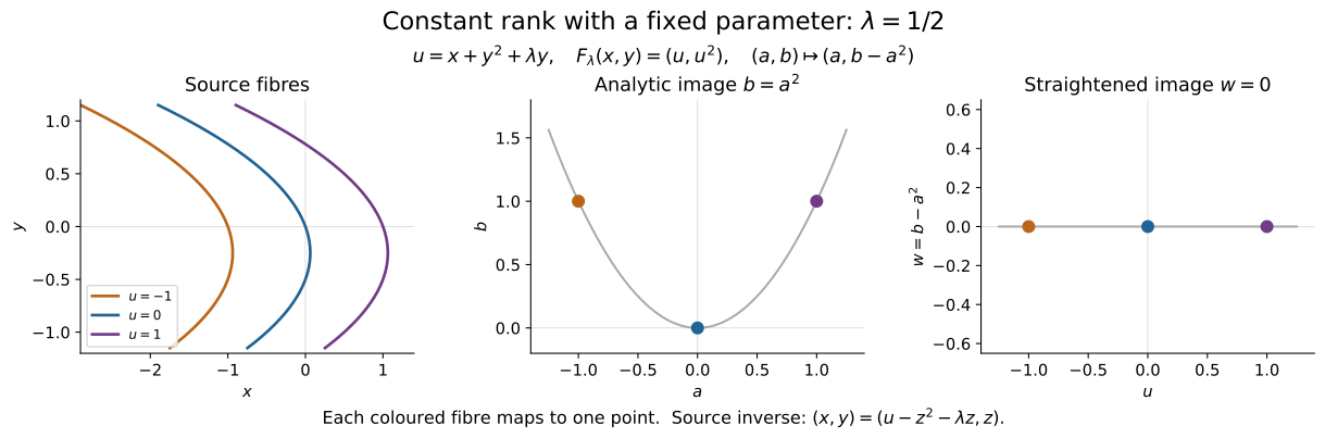
The example uses the source coordinates and target change displayed above. At the fixed parameter shown, each coloured fibre maps to its matching point on the parabola; subtraction of the square of the first coordinate puts the image on a straight line. The coordinate calculation proves the identity for every parameter, not only the plotted one. Full-size diagram · Reproducible Python source.
From a local analytic presentation to analytic curve selection
The human treatment of curve selection and Łojasiewicz inequalities, adapted from Guillaume Valette’s 2025 survey under CC BY 4.0, gives its arguments in globally subanalytic Euclidean spaces. Its cell-decomposition and Puiseux prerequisites are stated explicitly. The following chart argument explains how its curve-selection proof applies to the local sets in this lesson.
The companion analytic finiteness treatment now proves a prerequisite for that cell construction: real analytic Noetherianity via the existing Demailly division provider, Artin–Rees and Krull intersection, convergent replacements of formal linear solutions with prescribed jets, a finite Taylor family with analytic units, and the signed uniform-order normalization. The full analytic-composition and inverse-power reduction remains distinct from this finiteness proof.
Local comparison. Given and a subanalytic with presentation (1) near , there is an analytic coordinate neighborhood and a smaller bounded coordinate ball about such that the coordinate image of is globally subanalytic.
Proof. Choose the ball with compact closure inside both the presentation neighborhood and an analytic chart . For one of the finitely many maps in (1), the set is compact because is compact. Cover by finitely many closed coordinate boxes whose interiors cover and whose neighborhoods lie in . This follows by first choosing such a box around each point of and then taking a finite subcover. In their coordinates, each is a compact rectangle and the coordinate functions of are analytic on a neighborhood of that rectangle.
The graph of in these coordinates is bounded and semianalytic in its whole ambient Euclidean space: on a neighborhood of the box it is given by the rectangle inequalities and analytic graph equations; away from the closed box it is locally empty. A bounded ambient semianalytic set is globally semianalytic. Indeed, compactification is an analytic coordinate change on a neighborhood of its compact closure, whose image stays strictly inside the unit ball. The compactified set is therefore semianalytic, and is empty near the compactification boundary. In the projective-product convention of the preparation theorem, boundedness makes the compact closure lie entirely in the finite affine chart; the set is empty near every point at infinity, so is globally semianalytic there as well.
Projecting this graph proves that is globally subanalytic. Every point of has a preimage in , so
This is a finite union and intersection of globally subanalytic sets. Apply the same argument to every map in (1), and then apply the globally subanalytic Boolean-operation theorem to its finite differences and unions. The result is precisely .
The full two-sided curve. Suppose . Apply the cited component’s proved choice-and-Puiseux argument to the bounded coordinate set . It gives an arc with endpoint , analytic across zero. Choose small enough that the power series and chart inverse are defined whenever . The analytic map
interpreted in the analytic chart, has and for every . If , it is nonconstant. This proves the exact two-sided statement from the local comparison and the explicit cell/Puiseux inputs; it imposes no global definability assumption on or .
No assertion of finiteness at infinity has entered this argument. For instance, is analytic locally but cannot be globally subanalytic: intersecting with the horizontal axis and projecting would make its infinite discrete set of zeroes a definable subset of the line, contrary to finite cell decomposition. Each bounded chart piece nevertheless has the local comparison just proved. The ambient local finiteness and properness qualifications elsewhere in this lesson therefore remain in force.
Removing the unit from a resolved function
A resolution is often expressed with a nonvanishing analytic factor: . The precise sign-only expression (2) follows from that form near a point of the zero set. This last coordinate step changes neither the map nor its isomorphism over .
Unit normalization. Suppose a nonzero analytic function has the displayed form near a point where its value is zero. There are analytic coordinates centred at in which it is a sign times a monomial. The coordinate change preserves the normal-crossing coordinate hyperplanes through .
Proof. Any factor with is a local analytic unit; absorb it into . Centre the remaining coordinates at . At least one active exponent is positive, since the function vanishes there. Relabel it . Shrink so that has constant sign . The positive function has a positive analytic -th root . Indeed, the implicit function theorem applied to has nonzero derivative in at its positive root. Set
The Jacobian determinant at the centre is ; all extra derivatives in the first row carry the factor . The analytic inverse function theorem supplies a coordinate change. Substitution gives . Because never vanishes, , and the other active hyperplanes are unchanged. This proves every claim.
The zero-set qualification matters. A nonconstant unit such as has no positive vanishing exponent to absorb it and cannot become the constant monomial by an invertible coordinate change. In the resolution input, points of lie above , so the needed qualification holds. This coordinate argument supplies the last step from a unit-monomial resolution, not the construction of a singular-locus-preserving resolution itself.
Reducing marked equations to their coefficients
The source for the following coefficient construction is Edward Bierstone and Pierre D. Milman, Canonical desingularization in characteristic zero by blowing up the maximum strata of a local invariant, author manuscript of 25 November 1996, Proposition 4.12, Construction 4.18 and Proposition 4.19, with the proofs on pp. 33–34. The edition cited here is the complete 70-page author manuscript. The argument uses a distinguished derivative to select a hypersurface and transfers each marked order to finitely many coefficients on it. Ordinary permissible blowings-up divide by the exceptional coordinate with the assigned weight; exceptional tests pull back without that division. Keeping these two transformation rules separate is essential to persistence.
Our real analytic proof uses a convergent implicit coordinate change, then verifies coefficient divisibility along the whole smooth centre, the ordinary charts, the omitted transverse direction and the two other test transformations. Its hypothesis that the transverse direction is compatible with the existing exceptional hypersurfaces is exactly the additional hypothesis needed in the source’s Proposition 4.12. The conclusion is a local reduction with finite persistence under those hypotheses. The residual invariant, exceptional history and choice of centres in the surrounding desingularization construction require further arguments, identified after the proof.
Let be an analytic coordinate neighborhood, with coordinates , and let be a finite nonempty collection of analytic functions with positive integer marks. Its equimultiple locus is
The order of the zero germ is infinite. Assume that at a chosen , one distinguished pair satisfies and . If exceptional hypersurfaces are present, assume they are coordinate hypersurfaces in the variables. Thus the distinguished transverse direction is compatible with them. This is an explicit hypothesis when exceptional divisors have already appeared.
Coefficient reduction and persistence. After an analytic change of the transverse coordinate, there is a smooth hypersurface , transverse to these exceptional hypersurfaces, and expansions
Here and . In a neighborhood of ,
The orders on the right are computed on . If a smooth centre has normal crossings with the exceptional hypersurfaces and , this equality persists near every point above where the transformed marked equations still have their marked orders. In a chart with exceptional coordinate , the coefficients transform with their own marks:
The hypersurface transforms strictly, with local equation . Its transforms remain smooth and have normal crossings with the transformed exceptional hypersurfaces. The same coefficient reduction also persists under adjoining an independent variable and under an exceptional blowing-up in two existing exceptional hypersurfaces. For the latter test transformation the functions are pulled back without dividing by an exceptional power. Repeated applications give the corresponding assertion along every finite sequence of these transformations, at points satisfying the marked order conditions.
Proof of the initial reduction. Put . Its derivative with respect to is nonzero at , so the analytic implicit function theorem gives as a graph . Replace by , leaving unchanged. Shrinking the neighborhood, with an analytic unit. Differentiation in the new coordinate is the same as differentiation in the old one with held fixed. The exceptional coordinate equations are unchanged.
Taylor expansion in , with analytic remainder, gives the displayed expansions. Since , . The coefficient is nonzero. If the order of at a nearby point is at least , its derivative vanishes there. Thus every point of lies on .
At , expand each coefficient in . Terms with distinct powers cannot cancel. The remainder has total order at least . Consequently,
This proves the equality of loci. The distinguished coefficient also shows that the order of at any point of this locus is exactly .
Divisibility along a permissible centre. Straighten inside , keeping as transverse coordinate and the exceptional equations as coordinate equations. Locally,
Write on . The coefficient conditions hold at every point of , not merely at . Hence . To see this directly, expand a coefficient in the normal variables , , with analytic coefficients in the tangential variables. Every normal derivative of total degree less than vanishes at every point of , by the order condition there. All the corresponding tangential coefficient functions are therefore identically zero. This proves membership in the stated ideal power and makes every division in the transform formula analytic.
The ordinary blow-up charts. For , the chart is
Substitution and division give
The strict transform is . In the distinguished equation the coefficient of is zero. Near any point above ,
for an analytic . The factor in parentheses restricts to the nonzero constant on that exceptional fibre. It is a unit locally. The distinguished -th derivative is likewise nonzero there. The initial coefficient argument therefore applies to : its equimultiple locus lies on and equals the locus of the displayed coefficient conditions with marks .
The remaining points above must be checked in the chart. Here , for , and the other are unchanged. A point in this chart that belongs to no chart has for every . Since , the quotient restricts to zero at such a point. The transformed therefore has value . Its order is zero, so that point is outside the transformed equimultiple locus. This covers every projective direction. If is empty, all lower coefficients vanish identically and this same -chart argument removes the whole marked locus.
In the charts, the new exceptional divisor is ; each surviving old exceptional divisor is another coordinate hypersurface in the variables. Together with they have normal crossings. This proves the geometric assertion as well as the coefficient formula.
The two other test transformations. An independent product variable changes none of the expansions, orders or equations. For a blowing-up of two exceptional hypersurfaces, choose equations . In the relevant chart the substitution is , with unchanged. The controlled test transform is now , so . Pullback cannot decrease the order of a coefficient at a point above : substituting analytic germs vanishing at into every Taylor monomial preserves its minimum degree. The distinguished coefficient remains a unit and . Thus the same order-locus equality and the transverse coordinate equation hold. The other chart is identical with the two exceptional coordinates interchanged; the prescribed distinguished point of an exceptional test is included in these charts.
After any of the transformations, the data again satisfy the initial hypotheses at a point where all marked orders persist. The distinguished order is exactly , the distinguished derivative is nonzero, and the coefficient expansions and exceptional coordinate equations have the required form. Applying the argument successively proves persistence for every finite allowed sequence.
This is the local dimension reduction: it replaces conditions on functions of variables by weighted conditions on functions of variables. The later sections prove recovery of divisor orders, the recursive history and coefficient construction, closed canonical centre selection, compact-local termination, and overlap compatibility. A multiplicity drop alone also need not give normal crossings with the exceptional divisor, as the cusp exercise below demonstrates.
Gluing canonical local resolutions into a proper global map
A function-resolution construction must fit across coordinate neighborhoods. The same Bierstone–Milman author manuscript, Theorem 13.2 and the proof of Theorem 13.3, passes from resolutions on relatively compact open sets to a global analytic map by unique compatible lifts. Its proof relies on the previously constructed invariant and local algorithm. Theorem 13.4 then treats the stronger requirement of a locally finite sequence of global blowings-up by extending and resolving centres.
The lemma below isolates the descent argument: the local proper maps and their isomorphisms over the full overlaps are hypotheses. Density forces uniqueness and the cocycle; quotient charts give the manifold; a finite compact-cover argument proves properness. This supplies the gluing step once compatibility exists, while leaving the construction of compatible local resolutions and the extension of centres to their separate proofs.
Gluing lemma. Let be a real analytic manifold with a countable locally finite relatively compact open cover , and let be closed. Suppose that each has a proper surjective analytic map from an analytic manifold, an analytic isomorphism over , with dense in . Suppose also that for every overlap there is an analytic isomorphism
Then these maps glue to an analytic manifold and a proper surjective analytic map , an analytic isomorphism over all of . If an analytic function pulls back under every to an analytic unit times a coordinate monomial near , the same holds for .
Proof. The overlap isomorphisms are unique. On the dense open inverse image of , any such isomorphism must be . Two continuous maps to the Hausdorff manifold that agree on this dense set agree everywhere: their equality set is closed, being the inverse image of the diagonal. Density restricts to every open overlap. In particular,
on their respective domains. The last equality follows by comparing both maps over a triple overlap. Thus the required cocycle is a consequence of uniqueness.
Take the disjoint union of the and identify a point of with its image under whenever its base point belongs to the overlap. The cocycle shows that each injects into the quotient, that its image is open, and that the induced topology and analytic charts there are its original ones. More precisely, the preimage over of this quotient is precisely : every representative over has a unique representative in that chart. The therefore descend to a map with .
The quotient is Hausdorff. If two points have different base points, disjoint base neighborhoods separate them. If they have the same base point, choose containing it; both points lie in the same open Hausdorff chart , which separates them by open subsets of the quotient. It is second countable because it is the union of countably many open second-countable ; the union of their countable bases is a basis. The analytic transition maps now make an analytic manifold. The map is analytic and surjective by its local descriptions.
To check properness, let be compact. Choose finitely many open neighborhoods covering , with each compact closure contained in some . Such neighborhoods exist by local compactness and regularity of a manifold. Each is a compact subset of that . Hence
is a finite union of compact subsets of . This proves properness. Merely gluing maps that are proper over smaller pieces, without control over their full inverse images on overlaps, would not justify this step.
Over , the local inverses agree on overlaps, so they give a global analytic inverse. The coordinate monomial expressions are local statements in the charts , and therefore remain true on . If on , the preceding unit-normalization lemma gives the exact sign-only expression near every point of , while preserving the map itself. This proves the lemma.
The density hypothesis makes the canonical transition unique. For a local construction by blowings-up, it is supplied by the dense complement of the exceptional sets in the coordinate charts. The later centre, termination and independent-tower comparison theorems construct the local maps and their full-overlap isomorphisms required here. The gluing proof does not turn the global map into a prescribed sequence of global blowings-up: that stronger construction has its own extension-of-centres argument.
Why the real zero set does not determine the resolved function
The function
has the two coordinate axes as its real zero set. They already cross normally. Nevertheless, is not a unit times a coordinate monomial at their intersection, even after an invertible analytic coordinate change.
Proof. At a nonzero point of either axis, the other factors are units, so the order of vanishing along that branch is one. If a coordinate monomial had exactly these two branches, each exponent would consequently be one. Its order at their intersection would be two. But the displayed has order four at the origin. The order of an analytic germ is unchanged by an analytic coordinate change: its first nonzero homogeneous term is composed with the invertible linear part of the change and remains nonzero in the same degree. Multiplication by an analytic unit does not change that degree either. Thus the two orders contradict the proposed monomial form.
The missing factor vanishes at the crossing, although it contributes no additional real branch. Resolving only the pictured real support loses this information. One real analytic blowing-up of the origin resolves this particular function:
The factor is a positive analytic unit. The other chart gives the corresponding expression at the vertical direction. The following exercise proves the complete proper-map and isomorphism assertions, rather than treating one affine substitution as the whole resolution.
Keeping the whole function through a resolution
A resolution of a function retains its vanishing multiplicities. Resolving only the reduced real zero set does not supply this information. We first prove the complete-function calculation for a supplied tower of blowings-up, identify the centre condition which protects the original regular-zero locus, and carry out a complete cusp example. The canonical construction and termination theorems later in the lesson supply such towers in general.
The ideal-theoretic endpoint is treated in Edward Bierstone and Pierre D. Milman, Canonical desingularization in characteristic zero by blowing up the maximum strata of a local invariant, complete author manuscript of 25 November 1996, Remark 1.8 and Theorem 1.10, pp. 7–8. The principal-ideal calculation below explains directly why an endpoint with unit weak ideal gives the required multiplicities of the actual function.
The total exponent belongs to the function
Let be a finite-dimensional Hausdorff second-countable real analytic manifold. Let be analytic and not identically zero on any connected component. A supplied admissible principal tower consists of finitely many real projective blowings-up
with , and the following data. The centre of is a closed embedded smooth analytic submanifold of positive codimension. Disconnected centres are allowed; the conditions below are imposed locally on each component. Empty steps can be omitted.
There is a locally principal analytic ideal sheaf , with nonzero local generator , and a locally finite labelled family of distinct smooth analytic hypersurfaces with simple normal crossings. Initially and . For every , every point of , and every local equation of , the germ of is not divisible by . Equivalently, its restriction to the germ of is not the zero analytic germ. It may still vanish at individual points of .
The centre lies in . The point order is a constant positive integer on each connected centre component; this is independent of the generator, since multiplication by an analytic unit preserves order. The centre and the old divisors admit simultaneous coordinates: locally the centre is a coordinate subspace, and the divisors through the point are distinct coordinate hyperplanes. This is the normal-crossing condition used below.
Put . Its ideal is invertible. Define
where is a local generator of . Here denotes the ideal generated by the analytic pullbacks of sections of ; the negative power in (PF2) is multiplication by the inverse invertible ideal. When the centre orders differ between components, the formula is read with their locally constant values. The chart calculation below proves that the result is an analytic ideal, rather than merely a fractional one. Changes of or multiply by analytic units.
The updated family consists of the nonempty strict transforms of the old hypersurfaces, retaining their labels, and the components of , with new labels. The strict transform of is the closure of . We also record when the centre is Cartier; that records a divisor factor even when the underlying blow-up is an isomorphism.
Total-transform lemma. Formula (PF2) gives nonzero analytic weak generators. They have no factor from any germ of the updated divisor family, and that family has simple normal crossings. Locally the actual function has the equality
where is an analytic unit and only the hypersurfaces meeting the coordinate neighbourhood are included. The exponents are locally constant along the corresponding labelled hypersurfaces. The old strict-transform exponents are unchanged. At a new divisor over a connected centre piece,
The containment condition in (PF4) means containment of the local centre germ. A divisor meeting the centre transversely, without containing it, contributes no exceptional factor.
Proof of analytic divisibility and exact exceptional order. Work in simultaneous coordinates , with . A convergent expansion in the normal variables has the form
For , the normal derivative vanishes at every nearby centre point, because the point order there is at least . Thus is identically zero. In particular,
For a fixed centre point , its degree- homogeneous normal polynomial is nonzero. Otherwise (PF5) shows that every term in the Taylor expansion at has total degree at least , contradicting the exact point order.
The -chart of the real projective blow-up has coordinates and analytic map , for , with unchanged. Substitution in (PF5) proves the analyticity of (PF2). On the fibre over , its restriction is . This is a nonzero polynomial: dehomogenization in any one coordinate is injective on the vector space of homogeneous polynomials of this fixed degree. A nonzero real polynomial is not identically zero on any open neighbourhood of any finite -point. If the germ of at such a fibre point were divisible by , its restriction to would instead vanish on a neighbourhood. This contradiction proves that the exceptional equation divides none of these germs. The charts cover the whole projective normal fibre. For , the dehomogenized polynomial is a nonzero constant, so the argument includes Cartier centres.
Proof for the old divisors and the total exponents. In the same coordinates an old hypersurface containing the centre has equation . If , its pullback is and its strict transform in this chart is . If , its pullback is and its strict transform is absent from the chart. An old hypersurface not containing the centre has one of the tangential coordinate equations, say , and its pullback is the same equation. These descriptions exhibit and all nonempty old strict transforms as distinct coordinate hyperplanes. They prove the updated simple-normal-crossing assertion.
Suppose a weak generator vanished identically on the germ of an old strict hypersurface at some point. Its vanishing would hold on a small open piece of that hypersurface. Points of this piece off are dense, as is immediate from the coordinate description. At any such point the blow-up is an analytic isomorphism and is a unit; thus the original would vanish on an open germ of the original . That contradicts the assumed exclusion of every local divisor germ. This proves the assertion for old strict transforms as well.
Substitute the displayed pullbacks of old equations and into (PF3). Every containing old divisor contributes exactly one additional copy of its exponent to the power of ; the transverse ones contribute none. The remaining nonzero factors join the analytic unit. This proves (PF4) and the equality (PF3) by induction from , .
These are the actual divisorial multiplicities. Indeed, after removing from (PF3), restriction of the remaining factors to the germ of is a product of nonzero analytic germs: the weak generator has that property, the unit does, and every other coordinate equation does. The local ring of the smooth germ is an integral domain, as follows from convergent power series. The product is nonzero, so one further power of cannot divide the total function. At an intersection of divisors this divisorial order is distinct from the point order, which may be larger.
Division in (PF2) removes a factor from the weak ideal. Equation (PF4) retains that factor in the total function. Neither a reduced support nor a discarded unit is substituted for the equality of functions (PF3).
Cartier steps and the proper analytic map
Cartier lemma. Blowing up a closed smooth analytic hypersurface is canonically an analytic isomorphism. If its local equation is and has constant point order along it, then near each point of that hypersurface
The weak ideal becomes the unit ideal near the centre, while the total function retains the exponent .
Proof. The centre-divisibility argument (PF5) gives with analytic. If vanished at a centre point, the point order of would exceed ; hence is nonzero there and is a unit on a smaller neighbourhood.
The normal projective fibre of a hypersurface is , a point. Its sole incidence chart has coordinate map , with all other coordinates unchanged. The analytic map from the blow-up to the original chart is therefore the identity in these coordinates. These chart inverses agree on their overlaps because they are inverses of the same blow-up map. They give the asserted global isomorphism, including when the hypersurface has no global defining function. Formula (PF2) leaves the unit ; the total-transform identity retains . The newly recorded divisor need not be an exceptional locus of a nontrivial modification.
Properness and endpoint. Every blow-up in (PF1) is a surjective proper analytic map between manifolds of the same dimension. If the supplied tower ends with , then is proper and surjective, and (PF3) is a unit times a coordinate monomial at every point.
Proof. Near a centre of codimension , the blow-up is the incidence manifold Its chart has the coordinates already used, so its dimension equals that of , and its projection is analytic. Off the centre the projective coordinate is uniquely , giving an analytic inverse there; over a centre point the fibre is exactly . This proves surjectivity, including .
These local incidence descriptions also retain the manifold separation and countability conditions. Points with different images are separated by inverse images of disjoint base neighbourhoods; points with the same image lie in one Hausdorff incidence neighbourhood and can be separated there. A countable base-chart cover, with finitely many projective charts over each centre chart, gives second countability.
The incidence equations define a closed subset. For a compact set contained in such a coordinate neighbourhood, its full inverse image is a closed subset of the compact space , hence compact. The same assertion holds in an open chart disjoint from the centre, where the map is an isomorphism. Now let be any compact set. Choose finitely many compact coordinate neighbourhoods , each contained in one of these charts, whose interiors cover . The inverse image of is a closed subset of the finite compact union . It is compact. Thus is proper, and finite composition proves properness of .
At the endpoint every local weak generator is a unit, so it joins in (PF3). This is the asserted unit-monomial expression. The positive-codimension condition rules out an empty projective fibre; it is automatic for centres contained in the zero set of a nonzero analytic germ. In dimension zero the original function is already a unit on each point, and the identity map suffices.
At a zero of the total pullback, the preceding unit-normalization lemma gives a sign times a coordinate monomial, preserving its crossing hyperplanes. At least one exponent is then positive, as required by that lemma. Away from the zero set a nonconstant unit need not become a constant under an invertible coordinate change.
The original regular-zero locus is protected
Set
The centre hypotheses above do not by themselves make the tower an isomorphism over . For , the origin is a smooth constant-order-one centre with no old divisors, yet blowing it up introduces a projective line over a point where . Thus the centre-selection rule must enter the argument.
We use this precise additional condition:
(R) At a point where the weak generator has order one and no member of the current divisor family passes through the point, any chosen centre meeting the point has germ equal to the entire smooth weak-zero hypersurface there.
Centres also avoid the unit-ideal locus by the already imposed condition .
The full terminal-component rule has (R), with the following meaning of “full.” A chosen centre germ is a whole local component of the terminal equal-invariant stratum, rather than a smaller smooth submanifold merely contained in that stratum. Here is the entire calculation needed at an order-one point without old divisors. Take as an analytic coordinate, using , and present the weak equation with mark one. Its coefficient hypersurface is ; its sole coefficient below degree one is . There are no old-divisor entries. In the order/history notation, the word is therefore . After shrinking, every point of has exactly this word, whereas off the weak ideal is a unit. Thus its equal-word germ is precisely the single smooth hypersurface germ . A full local component through the point is itself, which proves (R). This verification assumes that the rule chooses a centre with the stated full-component property; it does not construct a global closed centre or prove compatibility of independently chosen towers.
Protected-complement lemma. Every supplied admissible principal tower satisfying (R) restricts to an analytic isomorphism at each stage.
Proof. We prove the assertion together with this local description over : the weak ideal is either a unit, or its generator is a smooth coordinate and the divisor family is empty near that point. Initially this holds because gives a unit and gives a coordinate by the analytic inverse function theorem.
Assume the description and the isomorphism through stage . At a point with unit weak ideal, the centre is absent on a neighbourhood, so the next blow-up is an isomorphism there and the ideal remains a unit. At a point with nonunit weak ideal, the generator has order one and there are no old divisors nearby. If the point is outside , closedness of supplies a neighbourhood avoiding the centre; the same description persists there. If the point belongs to , condition (R) makes that centre locally the full smooth weak-zero hypersurface. The Cartier lemma says that the blow-up is an isomorphism there and makes the weak ideal a unit. A divisor can be recorded in this last case, but the alternative “weak ideal is a unit” places no emptiness requirement on the divisor family.
These alternatives cover every point over , and the local inverses agree wherever their domains overlap because they invert the same map. They therefore give an analytic inverse on the entire inverse image of . This proves the induction and the conclusion for every finite composite.
Combining the endpoint and protected-complement lemmas gives the desired principal-function conclusion for any admissible tower satisfying (R) and reaching the unit weak ideal. The later compact-fibre termination theorem constructs these towers on neighborhoods of every base point. Their independent-tower comparison supplies analytic isomorphisms over full overlaps. The global assembly then applies the proper-gluing lemma. The total-function factorization and the isomorphism over pass through those comparison maps because they are local properties over the base. No uniform finite tower on the whole noncompact manifold is required.
Completing the cusp calculation
For , one has , so . The first blow-up makes the weak zero curve smooth but leaves it tangent to the first divisor. We keep both projective charts at each subsequent blow-up.
The first two charts, with their analytic maps to the original plane, are
The weak factor in the second chart is nonzero at every point of . In the first chart its zero curve is , tangent to at the unique meeting point . Blow up that point. The two charts over the first chart of (PF8) are
The order of the weak equation at the second centre is one, so (PF4) gives the new total exponent . The second chart of (PF9) has unit weak factor near each point of its exceptional divisor. In the first chart, the two old/new divisor axes and the weak line meet at the origin. All three are smooth, but three distinct branches at one point of a surface do not form a simple-normal-crossing divisor. Blow up that one point.
The two resulting charts are
Their composite maps to the original plane are, respectively, and . They also check the total pullback formulas directly. At the third centre the weak equation has order one, and both existing divisors contain the centre. The new total exponent is therefore , exactly as in (PF4).
The remaining weak curve is in the first chart and in the second. On their overlap, and , so these represent the same curve and its same meeting point with . The curve is transverse to . The old strict divisors meet at the other two distinct projective directions: at and at . The latter point is outside the -chart. At each final intersection, the two local branch equations have independent differentials; no three branches meet.
This also gives the monomial expression directly in each relevant neighbourhood. Near , use , with unit . Near , use , with unit , giving . At other finite points of in that chart, is a unit and only remains. In the other chart near , the unit is , leaving . These neighbourhoods cover the complete third projective fibre.
To check the entire surface, retain the unaffected -chart from the first blow-up and the unaffected -chart from the second. Together with the two charts in (PF10), these four charts cover . Their maps and complete functions are
| Final coordinates | in original -coordinates | |
|---|---|---|
For completeness, all six pairwise overlaps can be read from these blow-up coordinates. Domains are stated in the coordinates on the left; the inverse domain is stated in the last column.
| Transition | Domain | Inverse | Inverse domain |
|---|---|---|---|
Each pair consists of mutually inverse analytic maps on the displayed open sets. Substituting in the preceding table proves agreement of the original coordinates and of the total function. These transitions are composites of the three elementary blow-up transitions already given, so they obey the cocycle identities on triple overlaps. The zero values allowed by the stated domains are essential: for example, the / overlap includes , whereas the inverse formula in original coordinates would not be defined there.
In the first final chart the weak zero locus is disjoint from and smooth: on one has and . In the second it is disjoint from and smooth: on one has and . In each of the last two charts the weak curve and old exceptional component are disjoint parallel coordinate lines, each transverse to . At every point of , therefore, at most two branches of the total zero divisor meet and their local defining equations have independent differentials. This proves the simple normal-crossing assertion and all four displayed multiplicities.
All three centres lie above the origin. The properness argument proves that their composite is proper and surjective; it is an analytic isomorphism over . The unit-normalization lemma gives sign-only monomial coordinates at every point above the origin. Thus this example proves the complete function-resolution conclusion, with all multiplicities and every projective direction retained.
One may also continue to the unit weak ideal. The final weak-zero curve is a closed smooth analytic hypersurface, and it meets the existing divisors normally. Blowing it up is a Cartier identity step with weak order one. It records the residual-curve exponent and makes the weak ideal a unit everywhere, without changing the manifold or the total pullback formulas.
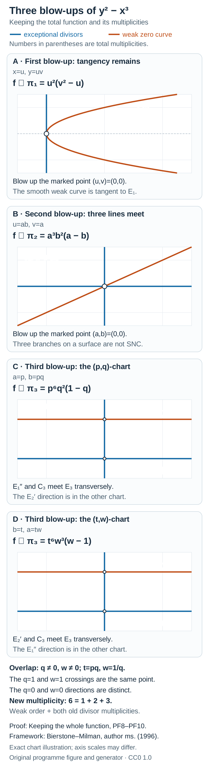
Open the full-size diagram · Reproduce the diagram.
Exercise: distinguish the weak order from the total order
At each of the three point centres, compute the weak order and the order of the complete function. Recover the new exceptional multiplicity, and explain why two point blow-ups do not suffice for simple normal crossings.
Solution. Initially the weak and total functions coincide, and has order two. Thus has multiplicity two. At the second centre , the weak factor has order one, while has order three. Its new exceptional exponent is . At the third centre , the weak factor again has order one, while has order six. Both old exceptional divisors contain that centre, so its new exponent is . After two blow-ups there are three distinct divisor branches at one point of a surface. An analytic coordinate change has an invertible derivative and preserves distinct tangent lines; it cannot turn those three branches into the at most two coordinate hyperplanes available in dimension two. The third point blow-up is therefore needed in this tower.
Exercise: identify the final curve and normalize the three crossings
Write for the final strict curve. Show that the whole curve is in the -chart and that restricts to . Find exact sign-monomial coordinates at the three points where meets , , and .
Solution. In the -chart a weak zero satisfies , hence lies in the overlap and has . In the -chart it satisfies , hence lies in the overlap and again has . In the -chart it has , hence lies in the -chart with . Thus the entire curve is covered by , with ; the direct map in the table gives . This is a computation on the resolved curve, not an assertion that the singular cusp is an analytic manifold.
Near , namely , set , . The positive real sixth root is analytic near , and the coordinate change has nonzero Jacobian. Then . Near , namely , set , ; this gives . Finally, near , write and set , . Since , this gives . All roots are taken only of positive units near the specified points, and each change preserves the displayed coordinate crossing hypersurfaces. No root is taken of the possibly zero exceptional coordinate.
Fixed-chart history and the first analytic resolution prefix
The local resolution invariant remembers when an exceptional divisor appeared. Its history must vary correctly over an entire fixed analytic chart, including points at which the present invariant value first appeared at different stages. The following argument proves that history step and its application to the first order/history prefix. It is a reconstruction of Bierstone–Milman, Canonical desingularization in characteristic zero, author manuscript, Proposition 6.6 and §§6.8–6.10, pp.36–37, with explicit analytic neighborhood witnesses. It does not construct the complete resolution algorithm.
Here a blowing-up is the real analytic projective blowing-up along a closed smooth analytic centre. Exceptional hypersurfaces retain labels recording their creation stage; a new exceptional hypersurface receives a new label. Labels follow strict transforms. At a point, only incident labels are counted. The initial exceptional family can be empty.
Fixed charts and history incidence
Fix a finite given tower of smooth analytic blowings-up with normal crossings between every centre and its current exceptional hypersurfaces. Work on a finite stack of coordinate charts Each map is the restriction of the corresponding blowing-up map. The charts are chosen before choosing pointwise presentations. On each chart, the centre is given by finitely many analytic equations and the finitely many exceptional hypersurfaces have analytic defining equations. Such chart stacks exist for a given finite tower: use coordinates adapted to the smooth centre and the normal-crossing divisor, then restrict a next-stage chart so its map lands in the preceding one.
For with , the set is a principal relative Zariski neighborhood of . Call a totally ordered invariant nonincreasing on fixed-chart neighborhoods if every has such a neighborhood on which . This definition does not assert local finiteness of all invariant values, or the stronger analytic threshold properties needed for the full noncompact algorithm.
Here is the ring of real analytic functions on the fixed chart. For an open subset , write These fractions are interpreted as analytic functions on . This ring need not contain every analytic germ at a point of .
History lemma. Suppose an invariant is defined at every stage of (AR1), is nonincreasing on fixed-chart neighborhoods, and satisfies:
- ;
- equality holds off the centre, where the map is an analytic isomorphism and the data are unchanged;
- takes one value on the entire centre portion . The chosen chart stacks must satisfy this condition at every stage.
For , let be its ancestor at stage , and set Let be the incident exceptional labels at . Call a label old for if it is the strict transform of a label already present at , and write for the old set. Then there is a neighborhood (AR2) such that, for every in it with ,
Proof. Induct on . At stage zero the old set is the initial incident divisor set; exclude the finitely many chart divisors not through by their nonzero defining equations.
At a later stage, take a finite product of analytic functions nonzero at to arrange the following conditions on one neighborhood (AR2). Pullback of an analytic witness at an ancestor is analytic on the current chart.
- , and at every earlier stage.
- , by including equations for all chart divisors that miss .
- The inductive old-set equality applies at whenever its value equals that at .
- Whenever , also . For this use one centre equation nonzero at and pull it back.
All products are finite and all their factors are nonzero at . Thus this really produces a principal relative Zariski neighborhood on the fixed chart; no arbitrary ordinary shrinking has been relabelled as Zariski shrinking. On the upper stratum put .
If , then The value therefore persists at both points. At each point the old labels are the incident strict transforms of the preceding old labels; the fresh exceptional label is not old. The inductive equality proves (AR4).
If both preceding values exceed , both birth stages are , so every currently incident divisor is old at both points. Again (AR4) holds.
It remains to handle Let . For every , monotonicity gives If , condition 4 excludes from the centre. If , constancy on the centre and the strict inequality do the same. Thus every step from to is an analytic isomorphism near the point and creates no incident exceptional divisor. All divisors incident at were already present at its birth, so . The drop at means , proving (AR4) in this last case.
The last case explains why birth times need not be locally constant. The incidence conclusion remains true because the comparison point acquires no new incident exceptional divisor during its longer constant-value history.
Put and order lexicographically. The lemma immediately proves that is nonincreasing on fixed-chart neighborhoods. On its witness neighborhood, its entire upper stratum is Indeed, a drop of the first entry makes the pair smaller, while equality of the first entry makes the old set a subset of ; equality of cardinalities then means that all these old labels remain incident. The complementary new labels satisfy on the upper -stratum.
Why analytic order satisfies the step hypotheses
The order of a nonzero analytic germ is the degree of its first nonzero Taylor term; a unit has order zero. It is unchanged by multiplication by an analytic unit. If is analytic on a coordinate chart and has order at , some coordinate derivative of degree is nonzero there. Where that derivative remains nonzero, every order is at most . Thus order is nonincreasing on a neighborhood of the precise form (AR2).
Here is the transformation calculation, including its hypotheses. Let the centre be in coordinates . Suppose has the same finite order at every point of this centre portion. The derivatives in the normal variables of degrees less than vanish at every . Taylor expansion in , with analytic coefficient functions of , therefore gives In a blowing-up chart write and for , , retaining . The quotient is analytic, by (AR8). Fix a point of the centre. The degree- Taylor term of there is a nonzero homogeneous polynomial in the normal variables alone: all terms of normal degree below vanished identically in (AR8). Consequently is a nonzero polynomial of degree at most . At every real projective direction in this chart its vanishing order is at most . Restricting an analytic germ to can only increase its order, so at every point over .
Equation (AR10) also shows that has no exceptional factor . Thus (AR9) is the strict transform of the principal analytic ideal, equivalently its total transform with the exceptional factor removed. To see the saturation assertion without assuming factoriality, if , restriction to gives . The ring of analytic germs on this smooth coordinate hyperplane is an integral domain, and the first factor is nonzero, so is divisible by . Cancellation gives ; iteration treats higher powers. This is the ideal-theoretic strict transform. No assertion identifying it with the closure of the real zero set is needed.
Off the centre the map is an analytic isomorphism, so order is preserved. We have therefore proved both step hypotheses of the history lemma for the order of a principal analytic ideal along a tower whose centres have constant current order. Each finite stage has charts with one analytic generator of this ideal; these charts can be chosen as part of (AR1).
The first order/history presentation on its full upper stratum
Set The history lemma applies to . For a marked analytic function , with positive integer , its marked condition at is ; for a finite family, impose every condition.
First-prefix proposition. Let be a point of positive order at a stage of a given order-constant SNC tower. There is a principal relative Zariski neighborhood on which , and the one family has marked locus exactly . Here is the fixed chart equation of . At every point of this locus, the same functions and marks give that point’s order/history family. Its remaining formal exceptional labels are precisely those members of incident at the point.
Proof. Multiply the history witness by a degree- derivative of nonzero at . On the resulting neighborhood, . Thus the first marked condition in (AR12) is equality of the order. Its remaining conditions say exactly that every old divisor at passes through . Equations (AR6) and (AR7) prove all assertions. Every function in (AR12) is analytic on the original fixed chart, so it also belongs to the localization .
This is a full upper-stratum statement, not merely an equality of germs at the selected point. Points where the order or the history count drops receive their own families. Unit points require no marking zero: the neighborhood misses the current hypersurface.
There is also an ordinary transformation check. Suppose a next centre lies in a constant -stratum and has normal crossings with the divisor. Near , (AR12) shows that it lies in every old divisor. The controlled transform of its mark-one equation is , a strict-divisor equation or a unit in a chart missing that strict divisor. The controlled transform of is (AR9), of order at most . If that order remains , the birth stage remains the same and the old divisors are exactly the incident strict transforms of the preceding old divisors. Hence the transformed family has its marked condition exactly at the points where persists. If the order drops, the first mark fails and the pair drops. This proves the claimed presentation behavior along ordinary admissible steps. Product and exceptional test transformations used later for coefficient-choice independence are a separate part of the full algorithm.
A residual extension once the common parent data exist
The next elementary lemma states its analytic inputs explicitly. The subsequent fixed-chart witness and higher-prefix theorems construct those inputs through the recursive invariant.
Suppose a parent prefix is bounded above by on a principal relative Zariski neighborhood . Suppose its entire equality locus there is the marked locus, on one smooth analytic coefficient manifold , of a finite family with common positive integer mark. Assume that these are valid common coefficient data at every point of that parent locus, and that on there are analytic identities where every remaining divisor equation restricts to a nonzero hypersurface germ on , and the incident restrictions are distinct normal-crossing coordinate factors on . Divisors containing , already consumed in the coefficient flag, are excluded from this product. The exponents are the exact common divisor orders at every point of the parent locus; absent divisor factors are units. Thus is a nonzero germ and has finite order at every point under consideration. Assume the next intrinsic residual value there is . The functions, coefficient manifold, and chosen coordinate derivations must be given by fractions of functions on the fixed chart with denominators nonzero on .
Let . Suppose a degree- coordinate derivative of one is nonzero throughout . It follows that there. Then is bounded above by on , and for its entire upper stratum is the marked locus of For there is no monomial pair. For , the parent and new upper strata coincide and are given on by . If all coefficient functions vanish identically on , the residual value is identically infinite there and the zero family remains the presentation.
Proof. At points where drops, the pair drops lexicographically. On the parent equality locus, the derivative bound gives . For a point of , put and . Multiplication of first nonzero homogeneous Taylor terms gives additivity of order, so the parent marked condition is exactly . On the new upper stratum , which implies the conditions (AR14). Conversely, (AR14) implies , so the point belongs to the parent equality locus. The derivative bound then forces . If , one residual function is a unit throughout, so the parent condition is just . The all-zero case is immediate from the stated identities.
The hypothesis about fractions is substantive. An analytic quotient in a germ ring is not automatically a fraction of analytic functions on a previously fixed chart. Nor do represented equations alone prove that they describe the intrinsic parent invariant on the full upper stratum. The first-prefix proposition supplies that semantic assertion at the first stage; further coefficient, quotient, history and test-equivalence arguments must supply it at each later stage.
Descent of matched analytic centres
One part of the algebraic resolution bridge, §5 has a direct analytic proof, under an exact matching hypothesis. Let be a countable open cover of a real analytic manifold , and suppose are closed smooth analytic centres of positive codimension, with normal crossings with the given exceptional divisor, and as embedded analytic submanifolds on every full overlap. Then is a unique closed smooth analytic centre in . Indeed, (AR15) gives ; its complement is open on each member of the cover and hence open in . Smoothness, analyticity and the normal-crossing property are local.
The corresponding analytic blowings-up glue. In coordinates with , the local map is the projection of Its chart has coordinates , for , , and the other ; thus it is smooth. It is proper over , since (AR16) is closed in a product with compact projective space, and is an analytic isomorphism off the centre.
Two local regular sets of generators of the centre ideal are related, near a centre point, by an invertible analytic matrix . The lifted change is . It is forced off the exceptional hypersurface, whose complement is dense in the displayed smooth charts, and therefore is unique everywhere. The lifts satisfy the cocycle and glue. The result is Hausdorff because points with distinct images can be separated in the base, while points with the same image lie in one open local blowing-up space. A countable cover gives second countability. Properness follows by covering any compact subset of the base by finitely many compact pieces contained in these coordinate neighborhoods. Controlled ideals and labelled strict divisors agree because their defining pullback and division operations agree on the overlaps.
This proves analytic descent for a finite sequence once the centre at every stage has been matched on every full overlap; identity stages can be inserted beforehand. It does not match independently chosen algorithms, choose a globally closed maximum stratum, or prove a locally finite bound on their number of steps.
The following sections extend these first-prefix arguments to the higher local invariant and its fixed-chart presentations. They then prove analytic closed thresholds and finite values on compact sets, choose closed canonical centres, establish compact-local termination, and compare independently constructed local algorithms before the global assembly.
What blow-up tests determine about a marked family
The next coefficient step divides out exceptional factors. To show that its numerical answer is independent of the chosen coefficient equations, we need to recover two quantities from the transformations those equations allow: their normalized point order and their normalized order along each labelled divisor. The distinction between ordinary and exceptional tests is essential. An ordinary test divides by the assigned exceptional power; an exceptional test in this argument uses plain pullback.
These tests come from Bierstone–Milman, Canonical desingularization in characteristic zero, author manuscript of 25 November 1996, Propositions 4.8 and 4.11, with proofs in §5, pp.31–33. We give the convergent analytic calculation, including the criterion along an entire divisor section and an explicit bound for stabilization.
Marked equations and what it means to compare their tests
Let be a smooth analytic germ of codimension in an ambient manifold at . A finite marked family consists of analytic germs on , with positive integer marks and . Its marked locus is
The zero germ has infinite order. Fix labelled smooth divisor germs in the ambient manifold which meet in distinct normal-crossing coordinate hypersurfaces. In particular, none contains .
We use the following operations on these data.
- An ordinary test blows up a smooth local centre contained in the marked locus and having normal crossings with the divisor family. On the strict transform of , replace by , where is a local equation of the new divisor. The centre-wide Taylor argument in Reducing marked equations to their coefficients proves this quotient analytic. Continue at points where all assigned marked orders persist.
- A product test adjoins a variable , pulls back the family, and records the divisor .
- An exceptional test string starts with such a product and a selected old divisor . Blow up the intersection of its strict transform with the most recently created divisor, repeatedly following the point on the strict transform of . Throughout this string the marked functions undergo plain pullback. In simultaneous normal-crossing coordinates these are ordinary analytic blow-ups of intersections of coordinate hypersurfaces; they need not have centres in (OR1).
After an exceptional string, ordinary and product tests are again allowed. The strings can be appended at intermediate stages, always starting a new string with its own product. No statement below requires unrestricted exceptional transformations with arbitrarily recomputed marks.
Two presentations with the same ambient germ, the same codimension , and the same labelled divisor germs are test equivalent here if their marked loci agree as ambient germs after every such allowed continuation, including agreement of the points at which an ordinary transform can continue. The presenting submanifolds need not be equal. This definition is stable under any allowed initial part of a sequence: further tests can simply be appended to it.
To calculate, one can make all marks a common positive integer . Choose a common multiple of the and replace
The order of a power is the exponent times the order of the original germ. Under an ordinary test its controlled transform is exactly the corresponding power of the old controlled transform; products and plain pullbacks also commute with powers. Thus (OR2) preserves every test, not just the initial locus. Multiplication by an analytic unit has the same invariance. All calculations below use integral powers of analytic functions.
Recovering the point order by measuring how many section tests remain
For common mark , write
Order-recovery lemma. The value , including infinity, is the same for two test-equivalent presentations of the same codimension. For this assertion ordinary and product tests alone suffice.
Proof. If , all functions are zero germs and the marked locus is the whole germ . Conversely, a marked locus which is a smooth ambient germ of codimension and is contained in must coincide with near : the inclusion of equal-dimensional submanifolds is a local isomorphism. Each then vanishes at every point of a neighborhood in , since its mark is positive, and is the zero germ. Thus infinity can be recognized from the common ambient marked locus and the codimension.
Suppose now . Take a product with a line and follow the arc . Blow up its endpoint times, each time following the lifted endpoint. In local coordinates on , centred at and adapted to the divisors, the chart following this arc has
This series converges on a small chart. Every exponent of is nonnegative, since . At the lifted endpoint its order is , hence at least . All the point centres and lifted marked points used in this calculation are therefore permitted. The point centres have normal crossings with the current divisor family. In this chart each old incident divisor remains a coordinate hyperplane, the most recent exceptional divisor is , and the preceding exceptional divisors from the point string miss the followed point.
The exact common power of in (OR4) is . Indeed, the restriction after dividing by that power includes the nonzero homogeneous degree- part of one , viewed as a polynomial in . That polynomial need not be nonzero at ; it is nonzero as a germ on the divisor, which is what exact divisorial order requires.
Let be the intersection of the latest exceptional divisor with the current presenting submanifold. Its germ is in (OR4). It lies in the marked locus as a whole germ exactly when . For sufficiency, every function is divisible by , so its point order is at least at every point of the section. For necessity, if the common power is less than , the nonzero homogeneous polynomial just exhibited is nonzero at points of arbitrarily close to the endpoint. The corresponding point order there is that smaller power; the entire section cannot be marked.
This section is recognizable without choosing . Any smooth germ of codimension in the latest exceptional hypersurface, contained in the ambient marked locus, lies in and has the same dimension as . It must equal as a germ. Thus two equivalent presentations identify the very same section whenever it exists. It is a permissible smooth centre, normal crossing with the other coordinate divisors.
Blowing up this section restricts to a Cartier identity on the presenting submanifold. Its controlled functions are nevertheless divided by . After such section blow-ups, the remaining common exceptional power is . Whenever a section blow-up is allowed, the lifted endpoint is still marked: the least point order there is this remaining power plus , and the remaining power is nonnegative. The next entire section is marked precisely when the remaining power is at least .
After a common section blow-up, the followed point for either presentation is still marked by this calculation. Equality of the transformed ambient marked loci forces the two lifts to coincide: each presenting submanifold has only one point over that endpoint, because its restricted blow-up is the Cartier identity. Thus the section tests really continue at common ambient points.
Consequently the observable successful section tests form the set
Here counts section blow-ups already performed after the point blow-ups. Every preceding section test in a successful pair also succeeds, by the same inequality. The set is empty precisely when . Otherwise it determines
The inequality in (OR5) proves the upper bound for the supremum. Taking for sufficiently large proves the reverse bound; these positive integers give pairs in and their ratios approach . All the operations defining and the test for its entire section are common to equivalent presentations. They therefore have the same value of .
Recovering one divisor order from an eventual slope
For an incident labelled divisor , set . Its normalized order is . Divisor order means the exponent of its local equation dividing the analytic germ; it is not the point order at an intersection of divisors.
Divisor-recovery lemma. If , every is determined by the allowed tests. Thus test-equivalent presentations of the same codimension have the same residual number . These statements also hold at any intermediate common marked stage of an allowed sequence.
Proof. Choose normal-crossing coordinates on with . After adjoining and performing exceptional tests following , the chart substitution is , for . Because these tests use plain pullback, their normalized point orders at are
Distinct monomials remain distinct under this substitution, so cancellation cannot alter the minimum. The transformed marked order stays at least , since pullback only adds nonnegative weights to the initial exponents. The two divisors defining every exceptional centre remain transverse coordinate hypersurfaces, so the full string is defined.
Put , over all the nonzero terms of the family, and let be the least among terms with . Both minima exist, as nonnegative integers, because at least one germ is nonzero. If , a term with has weight at least . Among terms with the smallest weight is exactly . Hence
The order-recovery lemma recovers each by appending its ordinary/product tests to the chosen exceptional string. The string itself is determined by the labelled divisor and the new product divisor. Equivalent presentations therefore give the same sequence , and so the same eventual slope. Repeating this separately for each label proves the assertion for . Starting all these tests after any common marked stage proves the stagewise statement as well.
For completeness, follows directly from analytic division. In simultaneous divisor coordinates, every Taylor monomial of every contains . Dividing out that integral monomial leaves a convergent analytic family after shrinking. Additivity of order in the convergent power-series domain gives . This is exactly the residual number used in (AR13)–(AR14). The tests establish its independence once coefficient families are test equivalent. They do not by themselves construct a coefficient family or prove the whole recursive equivalence.
Exercise: read an exceptional multiplicity from three tests
Take , coordinates , marked family , and labelled divisor . Compute its normalized point order and the normalized orders after exceptional tests following . Explain why using only the first exceptional test would give the wrong divisor order.
Solution. At the origin the point order is two, so . A product followed by exceptional tests substitutes and gives , without division by a power of . Its normalized order is . Thus , , and for every . The first difference is one, but the eventual difference is zero. The latter is the correct normalized divisor order: restricting to gives the nonzero germ , so no factor divides the original function. In particular, . The slope must be taken after stabilization; the changing minimum in (OR7) explains the misleading first test.
Analytic representatives on one fixed chart
A coefficient quotient may be analytic on a smooth germ without yet being represented by functions on the original chart. We now supply that representation, including when the divided monomial vanishes at the selected point. The analytic inputs are the programme proofs of Oka coherence and Cartan’s Theorem A. The latter is proved there from Theorem B, whose bump, approximation and inverse-limit arguments are supplied in that course. Thus the needed global section theorem has an explicit internal proof provider; it is not inferred merely from local coherence or from the existence of analytic quotient germs.
The maintained ring and the denominator lemma
Choose a conjugation-invariant complex polydisc , with real centre and finite positive radii, and put . The finite initial real analytic data are assumed to extend holomorphically to this polydisc; such charts can be chosen locally for any finite analytic input. Write Restriction embeds into the fixed real-chart localization . We maintain this stronger ring, rather than identifying either localization with the full analytic germ ring. Sums, products, nonnegative integral powers, quotients by represented units, and derivatives in the original coordinates preserve .
Finite denominator lemma. If and , there are such that
Proof. The sheaf is coherent by Oka coherence and the kernel theorem for coherent sheaves. The local membership hypothesis supplies a section germ of whose first coordinate is one. Cartan’s Theorem A expresses this germ as a finite -linear combination of germs of global sections of . At least one of those global sections has first coordinate nonzero at : otherwise evaluation of the first coordinate would give . Select it and divide by its first-coordinate value at , so that its first coordinate is one there. Its entries satisfy (AW2) as a global holomorphic identity.
The polydisc is Stein in the precise exhaustion sense needed by the provider. For example, is a smooth strictly plurisubharmonic exhaustion: its Levi matrix is diagonal with positive diagonal entries, and it tends to infinity at every boundary point. Theorem A therefore applies.
Finally reflect every entry by and average the section with its reflection. The row functions are in , so the averaged tuple is still in ; its first coordinate still has value one at the real point . All its entries are now in . This proves the real-witness statement.
Only one consequence of the section theorem was used: a global relation with first coordinate nonzero at the chosen point. Equivalently, it follows from , where is the coherent ideal of the point. The quotient is supported at ; its section represented by the local relation lifts by the cohomology exact sequence. The cited internal Theorem B supplies precisely this vanishing as well.
Division on the coefficient manifold
Suppose a smooth real analytic germ of codimension is defined by represented functions , with and independent differentials. Suppose where is an analytic germ on , is a nonzero germ, and . In the residual construction is a monomial with nonnegative integral exponents in divisor coordinates; it may vanish at .
Quotient lemma. There exist , with , for which In particular, the denominator representing is nonzero at . It contains no factor that one has merely assumed invertible because it is part of .
Proof. Since , the germs generate the same smooth-germ ideal as the , and their differentials at are independent. Complexify the real analytic identity in (AW3). In local holomorphic coordinates with , the germ of has an ambient lift . Hence vanishes on . A holomorphic germ vanishing there belongs to ; for instance Thus . Apply (AW2) to obtain the first identity in (AW4). On it gives . The local ring of a smooth analytic germ is a domain, so the nonzero germ can be cancelled. This proves the displayed representative for . The local lift , and the inverse coordinate map used to construct it, need not extend to ; their only role was to establish the local ideal membership to which (AW2) applies.
The same argument records zero identities. If restricts to zero on , there are , with , satisfying This is the certificate that makes a zero germ vanish on all of the subsequently chosen coefficient manifold inside a common principal open set. The ambient case of (AW4) also represents an analytic controlled quotient , where is a represented exceptional equation and is a nonnegative integer.
Represented coordinates and their derivatives
The quotient lemma does not authorize arbitrary local coordinates as elements of . We choose coordinates with representatives. Suppose represented functions on already have independent differentials there; these can include incident divisor equations and a retained transverse equation. The restrictions of the original ambient coordinate differentials span . Complete the given list using constant real linear combinations of those coordinates. With the defining equations , this gives an ambient list all in . Here denotes the original ambient coordinates. The analytic inverse function theorem supplies local coordinates, while the adjugate formula represents in . No global inverse of is asserted.
If coordinates adapted to a supplied smooth centre are needed, assume that its defining equations are represented as well. Retain the divisor equations which contain that centre, complete their conormal differentials by a subset of the centre equations, and complete the remaining tangent differentials by ambient linear functions while retaining the other divisor coordinates. The stated normal-crossing hypothesis gives the required independence. The chosen normal equations vanish on the centre and have its codimension, so their common zero germ is the centre germ. This is a represented adapted completion on the fixed chart.
The derivations annihilate the defining equations and satisfy . Their restrictions to are its coordinate derivatives. Quotient differentiation shows that every finite iterate applied to a represented function remains represented. These restrictions are independent of the chosen ambient representative because the derivations preserve the ideal generated by the .
For a fresh transverse choice, when the ordinary coefficient construction supplies a compatible tangent vector , choose the completing covectors so that all but the transverse one annihilate , while the transverse covector takes value one. This is possible when the retained divisor covectors annihilate , as required by compatibility. The resulting transverse derivation has value at . If a marked function has exact order and leading form nonzero on , its -th derivative in this direction is nonzero. Terms differentiating the vector-field coefficients involve lower derivatives of the function and vanish at . Consequently the coefficient construction’s defining equation and coefficients have representatives. The nonzero distinguished derivative certifies that the extra equation is independent. Existence and persistence of a compatible transverse direction belong to the coefficient construction; the calculation here preserves its representation once that geometric input is supplied.
One principal open set for all the finite witnesses
Consider one finite presentation at , with the quotient identities (AW4), any zero identities (AW5), and its finite coordinate flag. Multiply together all the following functions in : the denominators of its representatives, the factors in its quotient and zero identities, and numerator representatives of the nonzero Jacobian determinants used in (AW6). Include the distinguished derivative witnesses used for each smooth coefficient hypersurface. Every factor is nonzero at . Their finite product gives Every finite function belongs to , the selected Jacobians remain nonzero, and the global identities hold on the smooth coefficient manifolds cut out by these equations throughout . The represented coordinates are local coordinates at every point of those manifolds; global injectivity of their coordinate map is unnecessary.
There are two more finite certificates needed for residual orders. Suppose on a coefficient manifold the identities are , with , where the incident belong to its represented coordinate list.
First assume is the exact common divisor exponent at . Some residual has nonzero germ on . A derivative of its restriction in the other coordinate directions is nonzero at . That derivative is represented by (AW7). Include its nonzero numerator, as well as its denominator, in . At every point of , this tangential derivative remains nonzero. Therefore cannot be divisible by there. The common exponent is exact throughout that set. Repeat for the finitely many incident formal divisors. Divisor equations nonzero at may also be included in , excluding those labels throughout .
Second let , where orders are computed on the smooth coefficient manifold. Choose a nonzero coordinate derivative of total degree of one , and include its represented numerator in . Then For , this keeps one residual function nonzero. For an all-zero coefficient family, use (AW5) instead: it makes the family identically zero on , rather than inferring this from a zero germ alone. These are precisely the quotient, exponent and derivative witnesses required by the preceding residual-extension lemma. Identifying the parent invariant’s entire equality stratum, and the correct divisor histories there, is a separate semantic assertion.
Elementary division and its exact limit
There is a direct alternative to (AW4) when the coefficient manifold and divided factors are coordinates on the fixed polydisc itself. Suppose , and is a monomial in some of the remaining coordinate variables vanishing at . If is divisible by , with , then is divisible by . For each factor , the derivatives of of degrees below in that variable vanish on a neighbourhood of in . That coordinate slice is a connected polydisc, so the holomorphic identity theorem makes them vanish on the whole slice. Taylor expansion in the coordinate variables then shows that is holomorphic on the entire polydisc . Extend this function to independently of its first coordinates. This gives a global numerator with near . In particular this elementary argument handles division by an actual exceptional coordinate on a fixed blow-up chart.
It does not replace the quotient lemma for a general implicitly defined coefficient manifold on a previously fixed chart. Straightening that manifold produces local coordinates; it need not provide a global coordinate product or a global inverse coordinate map on that same chart. To illustrate the ring distinction, for the germ at zero is not with real analytic on and . Such an equality would give throughout by the identity theorem. At , the nonzero analytic function has finite order, so the right side grows faster than every inverse power as , whereas remains bounded. This is a contradiction. The example concerns arbitrary germs; (AW4) proves the stronger representation that is available for the particular quotients of represented data used here.
Finite analytic towers and the remaining resolution problem
For a supplied finite analytic blow-up tower, choose chart stacks whose analytic maps extend to holomorphic maps on the whole chosen polydiscs. They exist locally: choose coordinates adapted to each given smooth centre and its normal-crossing divisor, complexify the finite coordinate data, and shrink each next polydisc so that its map lands in the preceding one. A cover of each stage by such fixed stacks is enough. Once a stack is chosen, it is fixed before the pointwise coefficient recursion on its charts.
Pullback through such a map sends a global numerator or denominator on to one on , and preserves nonvanishing at the point over its ancestor. Equations for the currently listed divisor hypersurfaces are represented. Ordinary controlled divisions, divisions defining strict coefficient flags when the centre geometry permits them, and residual monomial divisions are represented by (AW4). Derivatives and coefficient restrictions are represented by (AW6)–(AW8). Integral powers used to clear marks preserve the same class. Therefore every finite branch made from these operations has represented functions and equations on its fixed chart, including branches rebuilt after an earlier invariant prefix drops. Different points and different branches may have different numerators and denominators on that same chart; no finite enumeration of all branches is claimed.
For transport along a persisting prefix, this statement applies to the actual data being transported. If an old-divisor count drops, the representation argument does not authorize retaining a positive-mark equation for a divisor now absent: the geometric recursion must transport its unadjoined family and then adjoin the currently incident old block. Representation preserves the inputs of that operation; it does not change the history rule.
This proves the fixed-chart analytic witness step using an existing internal analytic theorem, with a direct elementary proof for coordinate-monomial division as well. The higher-prefix argument below uses these witnesses. The analytic-threshold theorem then derives the topology and finite-value properties needed for centre selection; the compact-fibre and overlap theorems complete the tower construction. The total-function and protected-complement lemmas apply to those towers. The target remains an arbitrary-dimensional real analytic manifold.
Higher analytic prefixes, current history, and rebirth
We now continue the first order/history prefix through its higher coefficient and residual steps. This part concerns a finite given tower of permissible analytic blowings-up. It constructs the local word and its compatible local presentations, including points at which an earlier entry drops. The later centre and termination theorems use this local construction to produce the canonical towers themselves.
The argument uses three proved ingredients in this lesson: coefficient reduction and persistence, recovery of marked point and divisor orders by tests, and history incidence on fixed charts. For the fixed-chart conclusion it also uses analytic representatives on one fixed chart, with the analytic input stated there. The last ingredient supplies actual quotient and derivative representatives; the proof below supplies the missing assertion that they describe the invariant on the entire upper stratum of a principal relative Zariski neighborhood.
The human source comparison is Bierstone–Milman, Canonical desingularization in characteristic zero, author manuscript of 25 November 1996: Example 4.16 and the statements of Construction 4.23 and Proposition 4.24 are on pp.29–30; the coefficient and residual proofs are on pp.33–35; the recursive history construction is in §§6.9–6.15, pp.37–39. These are the page numbers of the 70-page author manuscript. We keep fixed marks during tests and distinguish them from marks recomputed at an ordinary stage.
Exact residual transport under an ordinary step
Let be a smooth analytic coefficient manifold and a finite labelled divisor family whose restrictions to are distinct normal-crossing coordinate hypersurfaces. No member of contains . Clear the marks of a finite nonzero family to one positive integer , and factor The division is analytic: in simultaneous coordinate series, every term of each has exponent at least in every divisor coordinate, and shifting those finitely many exponents preserves convergence on a smaller chart. No divisor coordinate divides all the . The residual value is , independently of the common mark, by the order-recovery result.
For , its normalized residual family is At least one residual function has its assigned order exactly, so this family has normalized order one. For , one residual function is a unit and the terminal family is . The all-zero coefficient family is the separate terminal value ; no common exceptional factor is assigned to it.
Suppose a smooth centre lies in the marked locus of (RX2) and has normal crossings with the divisor coordinates. Put , using the divisor germs containing the centre germ. The marked conditions along the whole centre give , and, when , . This is a centre-wide statement: expand in normal coordinates of ; their derivatives below the assigned degree vanish at every point of , so the corresponding analytic coefficient functions vanish. For the coordinate monomial the second membership is .
In a blowing-up chart with new exceptional equation , the controlled coefficient transforms factor as Both factors are analytic. If , the first is ; if , its analyticity follows from the monomial marked condition. Its new exponent is and the exponents of the old strict divisors are unchanged.
This is the exact common exceptional factor, not merely a possible factor. Choose of order at . The normal Taylor-polynomial argument in (AR8)–(AR10), applied to , shows that has order at most at every point over and has no factor . For an old strict divisor that is present, its complement of the new exceptional divisor is dense in that strict divisor germ. There the map is an isomorphism and a common old factor of all the would give a common old factor of all the original . That is impossible: one restriction to the old divisor is a nonzero analytic germ, and the analytic identity theorem makes it nonzero as a germ at every point of a sufficiently small connected divisor piece. Pulling to the strict transform preserves that property. If an old divisor equals the centre in , its strict transform is absent and makes no claim here.
Consequently the freshly computed residual value at a point over , whenever the preceding coefficient presentation persists, is Equality holds exactly where the transformed residual family has its marked condition. One direction follows from its marks. For the other, the preceding marked condition says ; if the second term is , it supplies the optional monomial mark . Thus at a persisting point the transported family is a valid fresh normalized residual presentation with its original marks. It need not be the literal choice of functions made by another presentation.
For , the residual unit pulls back to a unit, and has new exponent . The residual value stays zero wherever the parent persists. Zero coefficient functions remain zero; the infinite case needs no finite factor calculation.
Comparing residual presentations while their marks stay fixed
Two compatible coefficient choices for the same normalized parent family have the same ambient marked loci after every allowed test: each equals the corresponding transformed parent locus by the coefficient-persistence theorem, including its exclusion of irrelevant projective directions. The same conclusion holds for coefficient choices from two test-equivalent normalized parent presentations of the same codimension: compare each coefficient locus to its own parent locus, and then use parent equivalence. Their coefficient manifolds have the same codimension. The order-recovery result therefore gives equal normalized point orders and equal normalized orders along each labelled divisor, at the current point and at every common marked stage of a test sequence. It also identifies the all-zero case: the common ambient marked locus is the whole presenting manifold of that codimension, so both coefficient families are zero and give the same terminal value and germ.
Clear the two coefficient families to the same common mark . They now have the same integers and the same . We prove that their residual families (RX2) are test equivalent. During the test sequence retain a factor identity where is a unit. The initial marks remain fixed. At an intermediate exceptional test, need not be the greatest common exceptional factor.
For an ordinary centre in the transported residual marked locus, use exactly (RX3) with these fixed marks. The monomial exponents update by (RX4), with their current values. A product pulls back the factors and gives its new divisor exponent zero. In a distinguished exceptional-test chart, both factors undergo plain pullback. The new divisor exponent is ; the strict transform of keeps its exponent and that of is absent in this chart. No other divisor contains this intersection in the normal-crossing coordinates. These operations prove (RX6) along every allowed test string.
At a point of the transformed coefficient manifold let There is no infinite-minus-infinite subtraction: a nonzero analytic germ stays nonzero under these modifications and products, so and are finite in this branch. The transported residual condition is exactly For , the initially unit residual remains a unit. Each condition in (RX9) implies the marked parent condition .
We compare the two residual families by induction along a proposed residual test sequence. Their exponent ledgers agree initially. Outside the common coefficient marked locus, both residual loci are empty by (RX9). On that locus, append a fresh product and the order-recovery tests. The stagewise order-recovery theorem gives the same for both coefficient presentations. Their common labelled divisor incidence and equal ledgers give the same , and therefore the same conditions (RX9). An ordinary centre in this common locus is permissible for both coefficient presentations; its ledger update depends only on which common labelled divisors contain the centre. Products and exceptional strings also have the same updates. The induction proves equality after every allowed continuation.
This proves test-choice independence of the residual class with the full formal divisor set. It uses the marked-locus comparison of the parent and the proved recovery tests, rather than assuming that a residual class is canonical. It also explains why an exceptional test must not be followed by silently changing the residual marks to fresh ones: (RX9) concerns the transported marks.
Removing an old block while adjoining its current equations
We use a coordinate fact for nested centres. Suppose a smooth is transverse to a normal-crossing divisor family, and a smooth has normal crossings with that family in the ambient manifold. Its restriction to then has coordinates simultaneously adapted to and the restricted divisors. To construct them, retain the restricted equations of divisors containing among its normal coordinates; their differentials are independent. Complete them by equations of inside . The remaining divisor coordinates restrict independently to , and can be completed to coordinates there; extend them together with the chosen normal equations. The analytic inverse-function theorem gives the required coordinates. Extending by normal coordinates for , while retaining the ambient divisor equations, gives an ambient adapted system. Thus the centre charts used below are genuine simultaneous charts, not a consequence inferred from point orders alone.
Let be a labelled block of incident divisors, and put . For a residual family define Its marked locus is . We show that the class of (RX10) for the reduced formal set is independent of the compatible coefficient choice.
An ordinary centre in this locus lies in every divisor of . If it has normal crossings with the remaining divisor family, it has normal crossings with the full one. Indeed, on , the equations of are independent coordinates for their smooth intersection. Restrict the remaining divisor coordinates to that intersection, straighten the centre there while retaining those coordinates, and extend by the equations of . These coordinates straighten the centre with the full divisor family. The same argument, extended by normal coordinates to , gives the ambient statement.
The controlled transform of is a strict-divisor equation; in a chart missing that strict divisor it is a unit, so there are no continuing marked points there. A product preserves this description. An exceptional test permitted by uses two remaining coordinate divisors, and its centre is not contained in any old . Its plain pullback of is therefore a strict-divisor equation without an additional exceptional factor. Repeating these arguments shows that every reduced-set test of (RX10) is a full-set comparison test for its residual part, with the old equations enforcing the required intersections.
The residual comparison just proved, followed by intersection with these same ambient old-divisor loci, now proves equality of the two classes (RX10). This is the operation required by the recursion. We have not used a claim that deleting arbitrary divisors from an unadjoined residual family preserves every test equivalence.
Prefixes and the new history block
At stage let generate the principal strict-transform ideal. Set , stop if it is zero, and otherwise use the first history prefix already proved. Write the later prefixes as Only a positive finite receives a history count and a successor. A residual zero or infinity terminates the word. Comparisons are lexicographic, with for positive finite . If a word has already terminated, use that terminal shorter prefix in comparisons; do not invent further numerical entries.
Suppose the prefix , with its compatible coefficient class, has been constructed. Take coefficients on one more smooth maximal-contact hypersurface, clear the marks to , and use (RX1) to define . The coefficient-choice comparison and recovery tests prove that this number and its residual class with the current formal divisor set are independent of the compatible coefficient choice. The parent marked locus and (AR13)–(AR14) identify the new upper stratum. Under an ordinary centre where is constant, either drops above it, making smaller, or the coefficient presentation persists and (RX5) proves nonincrease of . Only after this step is justified do we define the birth of .
For a point with positive finite , let The old block consists of those currently unassigned labels in that were already present at . Set Earlier blocks persist by strict transform along a -constant ancestor suffix, because all their integer prefixes are then constant. The definition is consequently unambiguous, and the blocks are disjoint. At the birth stage every unassigned incident divisor is old for this new prefix, so .
There is no need to postulate a separate history lemma for an arbitrarily varying unassigned family. Apply the proved history lemma to using all exceptional labels, and denote its old set by . The definition is precisely On a principal relative Zariski neighborhood and the upper -stratum, the preceding integer prefixes are equal, so their already proved incidence identities give . The all-divisor history lemma gives the same formula for . Intersecting them proves Equality of the count holds exactly where every old divisor at remains incident. Thus adjoining their mark-one equations as in (RX10) gives the full upper-stratum presentation of . The reduced-set comparison above proves independence of its test class. Along an ordinary step, a drop of makes drop; when persists, no new divisor is old and the old count can only decrease. The old strict-divisor equations detect equality of that count.
Transport the unadjoined birth family when a count drops
The remaining existence issue is a compatible next coefficient hypersurface after the formal old block has been removed. A fresh transverse direction cannot simply be assumed for a family with an arbitrary existing exceptional boundary.
At , the normalized family has a function of order equal to its mark and the reduced formal set is empty. A nonzero leading homogeneous polynomial has a vector on which it is nonzero. Taking that vector as a transverse coordinate gives the nonzero assigned-order derivative required by the coefficient theorem. This constructs a maximal-contact equation for .
Transport without old-divisor adjunction along the -constant suffix from to the current point. Its fixed residual marks remain valid. Each centre is in its marked locus: the lower prefix persists and the residual value is the same. Equations (RX3)–(RX5) make the transported family a fresh residual presentation at each persisting point. The coefficient-persistence theorem transports its chosen transverse equation and proves that it remains regular and transverse to the divisors created in this suffix. These are exactly the reduced formal divisors , since that set was empty at birth. The original full boundary can still be retained as a comparison ledger, because the actual centres have normal crossings with the total exceptional divisor.
At the current point adjoin exactly the equations of the old divisors which are incident now: The same transverse witness still works after adjunction: its distinguished residual function has not been removed, and adding equations only reduces the marked locus. The full-boundary residual comparison and then (RX10) identify this class with the class formed from any compatible current coefficient choice. Thus a compatible coefficient representative exists and its next coefficient class is independent of that choice.
This order of operations is necessary when stays constant but drops. If an old divisor present at birth no longer passes through the current point, its transported mark-one equation is a unit. Keeping it would make the marked locus empty and would incorrectly discard the new, smaller history stratum. It is omitted from (RX16), while the unadjoined residual functions and their transverse witness are retained. This handles a drop of the history count without pretending that the half-prefix was born again.
The full upper stratum can have different birth times
We prove the fixed-chart semantic step; it is stronger than choosing ordinary neighborhoods separately at each point. Work with the fixed chart stacks and represented data supplied by the analytic-representative theorem. Finite products of denominator, Jacobian, derivative and divisor-incidence witnesses define principal relative Zariski neighborhoods. Quotient identities and zero identities hold on those neighborhoods. Every assertion about such a neighborhood below uses these witnesses; ordinary shrinking is used only when initially choosing the chart cover.
Assume first that the parent prefix has a common presentation on its entire upper stratum near . Choose its coefficient coordinates, transverse derivative and coefficient family. Include the nonzero transverse-derivative and Jacobian numerators in the witness product. The same coefficient theorem then applies at every point of that parent stratum in the resulting neighborhood. Its coefficient germs represent the already assigned parent class there. Include the exact-divisorial-order and residual-order derivative witnesses. The factor identities now give (AR13) at every such point with the actual residual number: its independence was proved above by the test comparison. The argument of (AR14) proves nonincrease of on the whole neighborhood and gives one common residual presentation on its entire upper stratum. Intersecting the history witnesses proves (RX15) there, hence the common marked-locus assertion for .
It remains to spread the compatible representative (RX16), since it was chosen using the reference point’s birth. Fix . Choose witnesses at the finitely many ancestors and pull them to the current fixed chart. On the upper -stratum they give, for every , Thus the comparison point’s value is constant over the same suffix beginning at , even if its earliest birth is earlier.
At stage , every unassigned divisor at belongs to its new old block. Apply (RX15) at that stage, using its history witness as well. It follows that at every comparison point in the upper stratum, This is the decisive conclusion: the comparison point may have an earlier birth, but it has no incident reduced formal divisor at stage . In the history lemma’s earlier-birth case, all its current divisors are already old.
The common residual family at stage is valid on that whole upper stratum. Include its selected order-exact transverse derivative in the witness product. It then supplies the same birth transverse equation at every ; (RX18) removes any formal-divisor obstruction to that choice. Ordinary coefficient persistence and (RX3) transport this one family and its transverse equation over the common suffix (RX17). The represented transform identities and nonzero Jacobians are valid on a principal neighborhood of the current chart. Consequently they give the same compatible family at every current comparison point. Divisors from the birth block which are absent at are excluded from this neighborhood by their nonzero current equations; the incident old ones obey (RX15). Current adjunction therefore gives exactly the family (RX16) on the whole upper -stratum.
If , the needed semantic assertions at stage were established by induction on the number of stages. If , the current common residual family and the history identity were just established before choosing the transverse direction. Thus (RX17)–(RX18) use no future prefix assertion. They close the different-birth case without assuming that an arbitrary ordinary neighborhood contains a relative Zariski neighborhood.
Earlier entries that drop, and the finite recursion
The construction is a double induction: first on the number of actual blowing-up stages, then on prefix depth at a stage. At stage zero there is no exceptional history. At later stages, all prefixes on the preceding stages are already defined. At the current point start with the current principal equation and the order/history construction (AR11)–(AR12). At each subsequent depth:
- take coefficients of the already constructed compatible current presentation;
- define the residual value and prove its choice independence and nonincrease;
- define its birth and unassigned old block;
- use unadjoined birth transport and current adjunction to obtain the compatible next presentation;
- spread its data over the whole upper stratum by (RX17)–(RX18).
The centres in the given tower are required to be locally constant loci of the prefixes already constructed on their stage and to have normal crossings with the total divisor. Equivalently, one constructs the word on a stage before checking the next given centre. No assertion selecting a global centre is hidden in this requirement.
If an earlier entry has dropped at a point, an ancestor’s higher family is not reused to define its new tail. That former family is needed only to detect the first strict lexicographic decrease. The current tail is rebuilt from the current lower prefix and its current birth. The pointwise representative theorem supplies the new finite functions on the same previously selected chart, even when the marks, divisorial exponents, birth stages and coefficient manifold differ from those of the former branch. At each equal upper stratum the argument above then supplies common representatives of the assigned classes. This proves existence at reborn points, not merely continuation on one ancestor’s persistent stratum.
Every nonterminal coefficient step lowers the dimension of its presenting manifold by one. In dimension zero an analytic germ is either a unit or zero. A marked point for positive marks cannot contain a unit among its equations, so its coefficient family is zero and the branch terminates at infinity. It can also terminate at residual zero or infinity earlier. Thus at each point the recursion has depth at most the ambient dimension. On the finite list of prefixes of the reference word, multiply the corresponding witnesses: at a comparison point the first differing prefix decreases, or every entry persists through the same terminal value. Rebuilt tails cannot reverse that first decrease. This proves nonincrease of the complete local word on fixed-chart neighborhoods and over ordinary permissible steps.
The same induction proves invariance under an analytic isomorphism of already matched labelled towers. Initial orders and ideals are invariant; coefficient/residual classes are independent of compatible choices; ancestor births correspond; and divisor equations differ only by units. It does not prove that independently selected towers match.
The terminal coefficient manifold and the total divisor
The formal divisor set excludes old blocks. Some excluded divisors eventually contain the coefficient manifold, so they cannot be treated as additional transverse formal divisors. A convenient choice of the coefficient flag keeps track of this geometry explicitly.
Call an old divisor pending until its equation has been used as an equation of the coefficient flag, and consumed afterward. Maintain ambient coordinates in which the current coefficient manifold is a coordinate submanifold, consumed old divisors are coordinate hypersurfaces containing it, and pending old divisors together with formal remaining divisors restrict to distinct coordinate hypersurfaces on it. Maintain a mark-one pair for every pending divisor in the chosen equivalent presentation.
If there is a pending divisor , use its own mark-one equation as the next transverse coordinate. This consumes . Every other pending equation can be retained as a different coordinate, independent of that transverse coordinate, so its coefficient family still includes . After clearing coefficient marks to , it includes . No formal remaining coordinate divides , and that function has order exactly . Thus, while any pending divisor remains after the coefficient step, the common exceptional monomial is a unit and the next residual value is exactly one. Its residual family keeps the same pending pairs, using the proved integer-power equivalence to write them again with mark one.
If there is no pending divisor, take the transverse witness supplied by the unadjoined birth transport. It is transverse to the current formal family, which now contains all divisors not already consumed. The next flag therefore has the required coordinate description. When an ordinary centre is encountered along a persistent prefix, it lies in the current flag and has normal crossings with the total divisor. The nested-centre coordinate fact above gives blowing-up charts inside the flag, extended by its normal coordinates. In these charts the strict flag stays smooth; consumed strict divisors still contain it; and the pending/formal strict divisors and the new divisor retain their coordinate description. Charts with no strict flag contain no persistent prefix points. A dropped old divisor is absent at the current point and is omitted as in (RX16). This verifies the flag induction along a persistent suffix as well as at a fresh birth.
At a terminal residual value, no pending old divisor can remain: the preceding paragraph would otherwise force that residual value to be one. Consequently all incident assigned old divisors are consumed and contain the terminal coefficient manifold; the remaining formal divisors are precisely its transverse coordinate divisors. In the infinite terminal case, all coefficients are zero and the equal-word locus is that smooth coefficient manifold. In the zero terminal case it is the marked locus of its coordinate monomial. The minimal coordinate components of that locus are therefore smooth and have normal crossings with the total exceptional divisor, including the consumed hypersurfaces which contain the coefficient manifold. The minimal monomial-centre calculation supplies their explicit decrease under a permissible local blowing-up. This proves the local permissible-component assertion; it does not extend a selected component germ to a closed global centre.
The conclusion is the local recursive presentation theorem for a finite given admissible tower, together with the fixed-chart upper-stratum and history-incidence assertions, under the stated analytic-representative theorem. Numerical histories are defined only on the actual ordinary tower. Product and exceptional tests prove equivalence of marked classes; they have not been assigned a new numerical history by convention. These results are the local input for the analytic-threshold, canonical-centre and compact-fibre termination arguments below.
The strict decrease at a minimal monomial centre
There is a concrete numerical decrease in the terminal monomial case. Let have analytic coordinates , let be nonnegative integers and a positive integer, and consider the marked monomial Zero exponents can be omitted. At a point , its order is . Therefore its marked locus is the union of coordinate subspaces where it suffices to take inclusion-minimal qualifying sets . This is a finite union in the coordinate chart. Each individual is smooth and has normal crossings with the coordinate divisor. The union need not itself be smooth, so it cannot automatically be used as one smooth centre.
Fix such a minimal and blow up . In its -chart, for , set , for , and leave the other coordinates unchanged. The controlled transform is exactly Its new exceptional exponent is nonnegative by (MC2). Minimality also gives , hence Thus the chart replaces one exponent by a strictly smaller nonnegative integer, leaving the other exponents unchanged. The charts for cover the entire projective normal fibre, including every direction.
More locally, define the weight at a point to be the sum of the exponents of the divisor components incident there. At any point over the chosen centre, the new divisor is incident; the -th old strict divisor is absent, and some other old strict divisors may also be absent. Formula (MC4) proves that this weight drops by at least one from the ancestor point. Off the centre the map is an isomorphism and the incident weight is unchanged. For , the underlying blow-up is the Cartier identity, and the assigned exponent still decreases from to .
Consequently, in a tower formed entirely from these monomial tests with a fixed mark , a chain of points can meet at most its initial incident weight many chosen minimal centres. In a sequence starting above one point, each step meeting a centre lowers a nonnegative integer, and the steps avoiding centres leave that integer unchanged. This is a termination statement along that chain. Choosing globally compatible centres for the full resolution invariant, and proving termination on a relatively compact region, still require the global construction; the pointwise decrease alone does not supply it.
Why the residual presentation must retain its monomial condition
The additional pair in (AR14) can exclude points arbitrarily close to the chosen point. The following polynomial example supplies actual common coefficient data and lets us compute both the parent stratum and its residual refinement everywhere on the coefficient manifold.
Use coordinates on , and let the two labelled exceptional hypersurfaces be and . They have normal crossings and are transverse to . For an integer , put
For , the residual family consists of the single function . Give every mark . Define the parent value for this example by . This is a concrete minimum-order parent, without any assertion that these data are the output of a full resolution algorithm.
The coefficient reduction is exact. The derivative shows on . If , then , so . At a point , the term and the Taylor series of , which is independent of , cannot cancel one another. Consequently
The coefficient family on is exactly ; the coefficients of are zero and impose no conditions. Thus its marked locus is the entire parent upper stratum . At the origin , every has order four, so this is indeed the upper stratum through . All functions and derivatives are polynomial on the one fixed chart, hence are fractions with denominator one; no extension of a germ quotient is being assumed.
The exceptional factor is exact. Each is divisible by . Its quotient is a nonzero polynomial in alone, so at every incident point it is divisible by neither the coordinate nor the coordinate . The common divisor orders along and are therefore exactly two. Where one of these divisors is absent, its coordinate factor is a unit. Both divisor restrictions are genuine, distinct hypersurfaces of ; neither contains .
Write, on ,
For , define
If , then on , because all the residual monomials are homogeneous of degree in the vanishing coordinates . Off , one of is a unit, so . For , one has everywhere. Additivity of orders now gives the exact parent condition
At the origin the residual order is , and is nonzero throughout , including the degree-zero case . This verifies the derivative bound in (AR14) on the whole fixed chart. On the parent stratum define the residual value . We compare with : a point outside already has a smaller first entry, so no residual continuation off the parent stratum is needed for this comparison.
The instructive case . Here
Since takes only the values , the parent upper stratum and the residual upper stratum are respectively
Indeed, off the residual order is zero, and the parent condition requires , which means . On the residual order is two, and the parent condition requires , which means or . The points of remain in the parent stratum but have residual value zero, so they leave the upper stratum when the new entry is added. In coordinates on , is the union of the -axis and the -axis; is the -plane.
Formula (AR14) gives the marked family
The first three pairs alone have marked locus , the entire -plane. The last pair imposes , leaving precisely its two coordinate axes . For any , the point lies in the residual marked locus , but has , , and . Thus it would be wrongly included if the monomial pair were omitted. Taking arbitrarily small shows that this is already an error of germs at the origin, as well as an error on the full upper stratum.
Retaining the actual exceptional exponents matters too. At , one has , , , and , so this point belongs to . Replacing by the squarefree pair would wrongly exclude it, because . The pair has the same marked locus as , since ; this changes the mark as well as the function. Replacing only the function does not preserve the marked locus.
Boundary comparisons. The same family gives the following exact comparison. The marked residual family in a row is when .
| Residual order at the origin | Parent upper stratum | Refined upper stratum | Additional monomial condition |
|---|---|---|---|
| is the complete presentation | |||
| None | |||
| None |
For , the residual function is the unit , so the parent condition is , exactly ; there is no mark-zero residual pair. For , the residual marked locus is , and on it automatically. This is exactly why no monomial pair is needed when . These statements concern the displayed common coefficient data and their order strata; they do not select centres, establish choice independence, or prove termination of a resolution algorithm.
Exercise: compare two positive residual marks below the parent mark
Keep the same functions with , and take first , then . Compute the parent and refined upper strata at the origin. Explain why the two positive residual orders lead to different upper strata, even though the residual marked locus is in both cases.
Solution. When , the residual marked family is , with locus , and the required monomial pair is . Since , the inequality means , or . Thus in . Off , the parent condition still requires ; on , it requires , again . Hence and .
When , the residual family is , again with locus . The monomial pair is now , so its condition is , equivalently or . Therefore . The parent condition off still gives , while on it is , giving . Thus and . The difference comes from the exact threshold , which is three in the first case and one in the second.
Exercise: a zero residual value within the same coefficient family
Return to , but choose the parent point . Work on the principal relative Zariski neighbourhood . Compute the residual order at and give the full upper-stratum presentation on . Explain why the residual mark two used at the origin cannot be reused at .
Solution. The function is a unit everywhere on , so throughout this neighbourhood. Its value is itself the nonzero degree-zero derivative required for the case . The parent condition is now exactly , or . Thus both upper strata through are , with , and the complete presentation is . The residual pair has empty marked locus on this neighbourhood, because its function is a unit. Reusing the origin’s residual mark would therefore delete every point of the actual upper stratum. The mark is the local residual order at the selected base point; the exceptional factor and the coefficient functions themselves have not changed.
Prefix-controlled denominators and well-founded words
The recursive construction gives nonincrease of the complete word under an ordinary permissible transformation. Rational entries alone would not imply that a decreasing sequence stops. We first prove the precise discreteness that the construction supplies, and then prove finite termination near each base point. The second argument must control whole maximum loci, rather than a single chain of points above successive centres.
The human-source comparison is Bierstone–Milman, Canonical desingularization in characteristic zero, complete author manuscript of 25 November 1996, proof of Theorem 1.14, pp.39–40. Those pages give the factorial denominator recursion and the two terminal decreases. The compact-fibre argument below supplies the finite maximum-locus bookkeeping explicitly. It uses the already proved analytic thresholds, recursive presentations and history transport, and the containing-label centre rule. The page references concern the 70-page author manuscript.
Write a positive-order complete word as where the entries before the terminal one are positive and finite. The order-zero word is the stopping value. The recursive coefficient dimension drops at every nonterminal step, so , with the fixed ambient dimension. Each history count is a nonnegative integer. At a fixed preceding prefix, the possible next numerical entries are ordered by ; there are no entries after a terminal entry.
Denominator lemma. For each finite numerical prefix define positive integers inductively by Then is an integer whenever the next entry is finite. This assertion applies at every stage, including a freshly recomputed tail after a prefix drop. In particular, its bound depends only on the preceding numerical prefix, and not on the number of previous blowings-up or the total number of exceptional labels.
Proof. Present the first order by the weak generator with mark , adjoining old divisor equations with mark one. All its marks are at most . Suppose a normalized presentation at the current depth has positive integer marks at most . Its coefficient equations have marks , where . Thus every such mark divides . Replacing an equation of mark by its power makes all marks equal to . These are integral powers, and (OR2) proves preservation of all the tests used by the construction.
Factor the exact common exceptional monomial out of this common-mark coefficient family. Its residual numerator , the least order of the residual functions, is a nonnegative integer, unless all functions vanish. Hence If or the family is zero, the construction is terminal. Otherwise the next normalized residual family has marks and, when , the additional monomial mark . The old divisor equations have mark one. Every one of these marks is at most , proving the induction.
During a constant-prefix part of a tower, residual transport keeps exactly these fixed marks; the formula is the transport formula, not a change of mark. If an earlier prefix drops, the recursive construction recomputes the tail from the current data. Applying the same induction to that new numerical prefix proves the same bound there. History changes add equations of mark one and therefore do not alter this estimate.
Well-foundedness lemma. Every nonincreasing sequence of complete words (TN1) in fixed dimension eventually stabilizes.
Proof. Its first entries are nonnegative integers and are nonincreasing, so eventually they are constant. If that constant is zero, the words have stopped. Otherwise the first history counts are then nonincreasing nonnegative integers and eventually constant. Once a prefix is constant, the next finite numerical entries belong to the fixed lattice , by the denominator lemma. A nonincreasing sequence in this lattice stabilizes: after its first finite term there are only finitely many lattice points between zero and that term. An initial infinite value can either remain infinite, terminating the word, or drop once to a finite value. A zero value also terminates the word.
When the next value stabilizes at a positive finite value, its following history count is again a nonincreasing integer and stabilizes. Continue through at most coefficient depths. This proves stabilization of the whole word, including its length. A tail can restart with larger marks or different old blocks when an earlier prefix falls; the proof first discards the finitely many falls of that prefix before treating its tail. It therefore makes no assumption that a higher entry decreases independently of the earlier entries.
This is a descending-chain assertion. It does not give a uniform denominator for all words, or a finite set of values on an arbitrary noncompact stage. The analytic threshold argument uses this assertion separately to prove finite image on compact sets.
Analytic thresholds and finite values on compact sets
The fixed-chart proof gives a principal neighborhood on which the invariant cannot increase. We now prove the stronger analytic conclusions needed to select a closed maximum locus: every upper threshold is a closed real analytic set, and the invariant takes only finitely many values on each compact subset of a finite stage. The argument does not require an open analytic chart to be a Noetherian topological space.
The same results are treated in Bierstone–Milman, Canonical desingularization in characteristic zero, the 70-page author manuscript of 25 November 1996, Lemma 3.10 and Definition 3.11 on p.21, the analytic discussion on p.22, and Definition 6.4 on p.35. The complex-analytic ingredients used below have existing proofs in Analytic germs, local parametrization and the Nullstellensatz, Proposition 1.2 and Theorem 4.1: a complex analytic germ has finitely many irreducible components, and an irreducible germ has a small representative containing a connected dense complex manifold. We first derive the uniform-neighborhood consequences actually required here.
From germ containment to one common neighborhood
Let be open, let be a closed complex analytic set, and let .
Uniform continuation lemma. There is an open neighborhood of , depending only on and , such that for every closed complex analytic subset .
Proof. If , choose disjoint from . Otherwise decompose into its finitely many irreducible germs. For each component choose a representative on a small neighborhood of , with a connected dense complex manifold , as provided by the local parametrization theorem. Shrink a common neighborhood so that is the union of the restrictions of these representatives. The larger chosen domains of the are kept inside .
Suppose the germ containment in (AT1) holds. Then contains a nonempty open subset of : the germ containment holds on some neighborhood of , and density of supplies points there. It is also a closed complex analytic subset of the connected manifold .
Such an analytic subset with nonempty interior is the whole manifold. Indeed, its interior is open; at a limit point of that interior take a connected coordinate neighborhood with finitely many local defining holomorphic functions. Each defining function vanishes on a nonempty open subset and hence identically by the identity theorem. Thus the interior is also closed, and connectedness proves the assertion. Therefore . Since is closed and is dense in , also . This proves (AT1) on the chosen . The neighborhood was selected before , so it works simultaneously for all such analytic sets. A zero-dimensional component is a point and satisfies the same argument.
This is the step that a bare assertion about Noetherian stalks does not supply. The individual germ containments may initially hold on different neighborhoods; continuation through the fixed finite branch representatives gives a single neighborhood for all of them.
Finite-equation lemma. Let be any family of holomorphic functions, possibly infinite. Its common zero set is closed complex analytic. More precisely, for each there are and an open such that
Proof. The ideal generated by the germs , , in the Noetherian ring is generated by finitely many of them. To see that the generators may be taken from the family, express a finite set of ideal generators as finite combinations of the and collect the finitely many functions occurring. Choose accordingly and put on . Every vanishes on the germ . Apply (AT1) with , using the same for every . This proves the inclusion from right to left in (AT2); the reverse inclusion follows because the selected functions belong to . The common zero set is closed as an intersection of closed sets, and (AT2) proves local analyticity. An empty family has common zero set and needs no equations.
Decreasing analytic sets stabilize near compact subsets
Compact stabilization lemma. Suppose are closed complex analytic subsets of one open complex manifold . For each compact , there are an integer and an open neighborhood of such that for every .
Proof. Fix . The ideals of analytic germs vanishing on form an increasing sequence in the Noetherian local holomorphic ring, so they stabilize at some . An analytic germ equals the common zero germ of its vanishing ideal: its own finite defining equations belong to that ideal. Hence for all .
Use (AT1) for . There is one neighborhood on which for every . The reverse inclusion is already in (AT3), so the entire chain is constant on after . Finitely many such neighborhoods cover . Taking the largest of their indices and the union of their neighborhoods proves the assertion.
The compact restriction is essential. In the unit disc, the sets , for , are closed discrete analytic subsets and strictly decrease forever. Their points accumulate only at the boundary of the disc. The lemma states eventual constancy near each compact subset of the fixed domain, with an index that may depend on that subset and that chain.
Holomorphic witnesses cut out the real upper thresholds
Let be the complete local resolution word on one finite stage of the given admissible tower. On a fixed chart stack, the analytic-representative theorem uses a conjugation-invariant complex polydisc and its real part . Combined with the recursive semantic proof, it supplies, for every , a holomorphic function , real on , such that The functions are finite products of the represented denominator, Jacobian, derivative and history witnesses. They can depend on . What matters here is that they are all holomorphic on the same previously fixed , rather than merely germs at their individual points.
For a value in the ordered value set, put Then Indeed, if , a nonzero with would contradict (AT4), so every function in (AT5) vanishes at . Conversely, if , the index occurs in (AT5), and excludes from that common zero set.
By (AT2), is closed complex analytic. Near each real point, its equations in (AT2) are selected from the , so their restrictions are real analytic equations. Thus is a closed real analytic subset of . This proves closed analytic thresholds before using any finiteness property of the invariant’s value set. It neither defines a resolution invariant at nonreal points nor assumes compatibility of an entire complex resolution algorithm: the complex sets are made directly from the existing real-point witnesses.
The equality (AT6) identifies the threshold intrinsically on each real chart. These sets therefore agree on real chart overlaps, proving that every upper threshold of is a closed real analytic subset of the whole current manifold. Here “real analytic subset” means a closed subset locally cut out by finitely many real analytic equations; no separate reduced-space structure is being asserted.
Why only finitely many words occur on a compact set
We use the order-theoretic conclusion of Prefix-controlled denominators and well-founded words: every nonincreasing sequence of possible principal-function words eventually stabilizes. Its proof uses the integer marks and the denominator bound determined by the preceding numerical prefix; it is not a property of arbitrary positive rational sequences.
Let be compact. If were infinite, it would contain a strictly increasing sequence . For completeness, a totally ordered set with no infinite strict decrease has a least element in every nonempty subset: otherwise successive smaller choices give such a decrease. Starting with the least element of an infinite subset and successively taking the least remaining element therefore constructs the asserted increasing sequence.
The sets of (AT5) are decreasing closed complex analytic subsets of the same . They strictly decrease on : choose with ; then This contradicts the compact stabilization lemma. Hence is finite.
Every point has a compact coordinate neighborhood whose interior contains it, so the values are locally finite. More generally, a compact subset of the current manifold is covered by finitely many open chart pieces with compact closures inside fixed chart stacks. Intersecting the given compact set with these closures produces finitely many compact subsets to which the argument applies. Their finite value sets have finite union. Thus the complete word takes finitely many values on every compact subset of any finite stage. In particular it takes finitely many values on any relatively compact open working domain whose closure lies in that stage.
On a nonempty working domain with finitely many values, a largest value exists, and its maximum locus is exactly restricted to that domain. It is therefore closed analytic in the working domain. Each value locus is locally a difference of two closed analytic threshold sets: in a finite local list, use its own threshold and that of the next larger occurring value. This does not make every value locus smooth; the terminal coefficient and boundary-refinement arguments are needed to obtain smooth centres.
Finitely many terminal component branches near a compact set
There is a more concrete finiteness statement for a maximum locus. Suppose is the maximum word on an open working domain , and let . For every compact , there are finitely many ordinary coordinate neighborhoods covering such that where each is a connected smooth coordinate submanifold and the listed branches are the maximal coordinate subspaces in that union. They have normal crossings with the total exceptional divisor.
To prove this, use the adapted terminal flag from the recursive construction at each . In the infinite terminal case the local equality locus is its smooth coefficient manifold. In the zero terminal case it is the marked locus of one coordinate monomial, hence the finite union of coordinate subspaces determined by inclusion-minimal exponent subsets of total weight at least its mark. The terminal flag includes the consumed old divisors, so this is a simultaneous coordinate description with the total divisor. Choose an ordinary coordinate box small enough that all these subspaces are connected and the description holds. Since is closed and is compact, is compact; finitely many such boxes suffice.
The centre and compact-fibre arguments below use these finite coordinate descriptions. Compact stabilization here concerns thresholds on one fixed finite stage; it is not applied across different ambient spaces created by successive blowings-up.
Choosing closed smooth centres and matching their restrictions
The terminal local geometry gives permissible component germs, but a union of crossing components is not a smooth centre. We now give an explicit choice that extends across charts and commutes with restriction. Its input is the complete local word and its terminal-component geometry proved above, together with the analytic closed-threshold theorem. Existence of a finite maximum procedure on relatively compact regions uses the separate termination argument. The component refinement is the one in Bierstone–Milman, Canonical desingularization in characteristic zero, complete author manuscript of 25 November 1996, Remarks 1.15–1.16 and 6.17, pp. 11 and 40; the restriction principle is also used in §13, pp. 65–67. Here we prove the required real analytic centre and overlap assertions explicitly.
Chronological labels and the precise inputs
Work at a finite stage of a principal analytic tower on a Hausdorff second-countable real analytic manifold . Its current weak ideal is locally principal, with a nonzero local generator on each connected coordinate neighbourhood. Let denote the complete order/history word. Its first entry is the nonnegative integer order of that ideal. The construction stops where this order is zero.
Give the exceptional hypersurface introduced by the -th blowing-up the label . One labelled hypersurface may be disconnected: it is the whole exceptional hypersurface of that step. Retain its label under strict transform, allowing its current transform to be empty. Different connected pieces born at that same step do not receive arbitrarily ordered extra labels. Each is a closed smooth analytic hypersurface where nonempty, and the family has simple normal crossings. At a point there is at most one local branch of any one . These assertions follow from the adapted blow-up charts and hold for a Cartier step as well. At stage the ordered label list is therefore There are finitely many labels even when a hypersurface has infinitely many connected components. Empty labels can be kept as zero entries.
We use the following already separated properties of the invariant.
- On the current stage, every upper threshold is a closed real analytic subset, and the values are locally finite. We perform centre selection on a working domain where a largest value is attained and the weak ideal is not everywhere a unit. Its first entry is then positive. Finite image is sufficient for the existence of this maximum; an attained upper bound is sufficient as well.
- Near a point of value , the set of points with that same value is the terminal locus of one common presentation. It is either a smooth coefficient manifold , in the infinite terminal case, or the union in the zero terminal case. Here is a positive integer, the are positive integers after omitting zero exponents, and the indicated are the remaining transverse formal divisors. All consumed old divisors contain . There are simultaneous analytic coordinates for and the total divisor. The terminal locus and every component in (CC2) are the actual equal-word germs, independent of the coefficient presentation.
- On a matched labelled tower, the word, its birth history, and its terminal locus are invariant under analytic isomorphisms. The controlled weak transform, coefficient presentations and history construction commute with restricting the tower to an open subset.
The last restriction assertion includes a harmless reindexing after steps whose centres miss that subset; we verify it below. The first property is an analytic topology input, not a consequence of a finite number of coefficients at one point. We do not assume that an arbitrary noncompact stage has a global maximum.
A component is identified by the divisors which contain it
Let on such a working domain. It is closed analytic by the first property. For a local component germ of at , define Containment here concerns the entire component germ, not just whether . Order these bit vectors lexicographically, with , so the oldest differing label has priority.
Component lemma. Distinct component germs at a point have distinct sets (CC3). In a sufficiently small simultaneous-coordinate neighbourhood, the label set of each component is constant along that component, and the component germs at any nearby point are exactly those of the displayed components which pass through that point.
Proof. In the infinite case there is just the smooth germ , so uniqueness is immediate. Its containing labels are exactly the consumed divisors; every other incident divisor restricts to a genuine coordinate hypersurface on , and therefore does not contain its germ. This description persists on a small coordinate neighbourhood.
In the zero case write for the labels of the consumed divisors. In the adapted coordinates, (CC2) is a finite union of distinct coordinate submanifolds. Inclusion-minimality of means that none of these submanifolds is contained in another. Its containing-label set is precisely An additional transverse coordinate hypersurface cannot contain : its coordinate remains a free variable there. The sets in (CC4) are distinct. Shrink the neighbourhood to exclude divisors absent at and to retain the coordinate description. The same argument at every point of a displayed component proves constancy of its containing-label set. The local components through a nearby point are exactly the members of this finite coordinate union which pass through it. Two distinct members cannot become equal as germs at an intersection, since their different free-coordinate directions remain different.
Define the extra entry and the extended word by The same germwise definition can be made at every point using its own upper equal-word germ. For centre selection we need it only on the largest-word locus . The component lemma makes the definition intrinsic. It does not require choosing a global irreducible decomposition of a real analytic set.
The maximum of the refinement is a closed permissible centre
Let be the largest bit vector attained on . It exists because there are at most possibilities, even if is not compact. Define
Centre theorem. The set is a nonempty closed embedded smooth real analytic submanifold of the working domain. At each of its points it is one entire local component of the terminal equal-word locus. It has normal crossings with the total exceptional divisor, the weak order is constant and positive on it, and blowing it up is an admissible principal transformation.
Proof. Fix and use the finite coordinate-component description of the component lemma. Write its components as with constant label vectors . At every nearby point , Every occurs at , so it is at most . Formula (CC7) shows that, on this neighbourhood, is exactly the union of the labelled . At most one such component exists, by the injectivity in the component lemma. Thus the germ of at every is either empty or one whole smooth coordinate component. It is closed analytic locally along . Since is closed in the working domain, points outside have neighbourhoods missing . This proves global closedness and embedded smoothness; no closure of a locally chosen component across a different invariant stratum has been taken.
The simultaneous coordinates show normal crossings with every exceptional divisor, including the consumed divisors which contain the coefficient manifold. The first entry of is one fixed positive integer , so the weak order is exactly at all points of . In particular lies in the zero locus of the weak ideal. It has positive codimension, because that nonzero principal ideal cannot vanish on an open subset of a connected coordinate neighbourhood. The centre-wide Taylor argument gives the analytic controlled weak transform. The standard analytic blowing-up charts preserve the total normal-crossing divisor, and the properness and Cartier lemmas apply.
The centre can be disconnected. Its entire union is smooth because the proof gives just one component germ at every point; arbitrary unions of crossing terminal components would not have this property. On the infinite terminal branch, the centre is the whole local coefficient manifold. On the zero branch, it is one of the minimal monomial components (CC2), so the strict decrease (MC4) applies in every persisting chart. In particular the centre theorem supplies exactly the full-terminal-component condition used in the protected-complement lemma.
More generally, on every threshold is locally the union of the displayed components whose label vector is at least , and is therefore closed analytic. The label entry serves to choose the component. Termination uses decrease of the primary word, or the terminal monomial weight while that word persists; it does not assume a well-founded decrease for bit vectors of increasing length.
For example, a local terminal monomial has locus . The containing-label vectors of its two components are and . If label 1 is older, (CC6) chooses , including their intersection, and not their crossing union. At the intersection the selected germ is still the whole smooth hypersurface .
Deleting empty steps preserves the history and label order
Let be an open subset of the original base of a finite tower, and restrict every stage to the inverse image of . If a centre misses that stage’s inverse image of , its blowing-up restricts canonically to the identity there. The weak ideal and all old divisors are unchanged there, and the new exceptional hypersurface has empty restriction. Every later strict transform of that hypersurface also misses the inverse image of .
Remove just these empty-centre steps. Inserting or removing them repeats or deletes identical local data in the ancestor list. For each prefix its earliest occurrence may receive a different integer index, but the divisors already present at that occurrence are the same. Thus its old block, currently incident old block, and birth-transported presentation are unchanged. Induction on prefix depth proves that the full word and all assigned old blocks agree with those of the shortened tower. This uses the actual ancestor definition of birth; it does not reset history at each restricted stage.
The remaining chronological labels are identified by their order of creation. Passing from their bit vectors to those of the unshortened tower inserts zero entries at the labels of empty steps. This preserves lexicographic comparison: the first position where two vectors differ is carried to the first position where their zero-padded vectors differ. Hence An open restriction can disconnect an exceptional hypersurface. All of those pieces retain the same creation label; they must not be assigned fresh arbitrary priorities.
Only empty-centre steps are deleted here. A nonempty Cartier centre can give an identity on underlying manifolds while dividing the weak ideal and introducing a recorded divisor. That data transformation is retained, on both sides of every comparison.
A maximum procedure commutes with open restriction
Call the following a maximum procedure on a working domain: while the weak ideal is nonunit somewhere, select (CC6) using the current data, blow it up, perform the prescribed weak and divisor transforms, and recompute the invariant with the resulting history. Assume that its current largest value exists at each step. The compact termination argument separately supplies the finite instances used for resolution.
Restriction theorem. Restrict a maximum procedure on a domain to an open subset and delete its empty-centre steps. The remaining steps are exactly the maximum procedure on , for as long as the procedures in question are defined. The equality includes the transformed ideals, old blocks and ordered boundary data, through the canonical analytic identifications of the blowings-up.
Proof. At a current stage, write and for the corresponding current inverse images of the original domains. Suppose that their data have already been matched. Let be the selected centre in . If , restriction makes this step empty and (CC8) applies. There is no local change to the data on .
If , the largest primary value on is the same as on : restriction cannot create a larger value, and the intersection supplies a point attaining the larger domain’s maximum. On that common maximum stratum, the largest component-label vector is also the same, by precisely the same argument. The local component germs and their containing labels are unchanged by open restriction. Therefore This also proves existence of the required maximum on at that step without a compactness assumption on . By the analytic blow-up restriction lemma, as real analytic manifolds over ; the exceptional and strict-divisor ideals correspond under this isomorphism. The controlled weak ideal therefore corresponds as well. Invariance on a matched tower and (CC8) give the same next word and ordered history. This is the induction step.
For a finite procedure ending with unit weak ideal, the restricted procedure also ends with unit weak ideal. It cannot finish all of its retained steps with an unresolved open subset left over, because the final ideal is the restriction of that unit ideal. Thus it is the complete finite maximum procedure there. In particular, larger-domain steps of higher value that are disjoint from cannot change when a lower local value will be processed or how its eventual centre is selected.
Independently constructed towers on overlaps
Suppose finite maximum procedures ending with unit weak ideals have been constructed on two open analytic domains and for restrictions of the same principal data. Write their real analytic composite maps as and . Restrict both to and delete empty-centre steps. They start with identical data. Their first nonempty centres are both the centre (CC6) of those data, so they agree. The canonical isomorphism of their blowings-up identifies the next data. Repeating proves by induction that every subsequent nonempty centre and transformed datum agrees. If one tower ends first, its weak ideal is a unit on ; hence no nonempty step remains in the other tower. With and , the final towers therefore give an analytic isomorphism This is an existence proof of the overlap map, obtained by matching centres of independently run procedures. It is stronger than the earlier statement that already matched centres have matching blow-ups.
The same argument applies to an analytic isomorphism between two open base domains carrying one principal ideal to the other. It identifies the initial orders and terminal germs, carries each selected centre to its counterpart, and lifts canonically at every step. Since the label rule uses only chronological order and no chart numbering, it is preserved by these lifts.
The comparison maps are compatible with further open restriction, satisfy , and obey on each triple overlap. One can see this directly from the functorial coordinate identification of each common blowing-up. Alternatively, the final maps are isomorphisms over the dense complement of the original zero divisor; any two analytic comparison maps over the base agree there and hence everywhere by continuity and the Hausdorff property. The dense unchanged locus proves uniqueness after (CC11) has supplied existence.
These results provide closed smooth centres on each domain where the maximum procedure is used and give the full-overlap isomorphisms needed by the proper-gluing lemma. For an arbitrary noncompact analytic base, the separate compact termination argument must first produce finite maximum procedures on an appropriate relatively compact open cover. The centre theorem does not assert a global maximum on that base or a finite sequence of global blowings-up. Once those finite procedures exist, (CC11)–(CC12), the total-function ledger and the protected-complement lemma have exactly the hypotheses needed for the proper analytic resolution map.
Finite termination over a compact fibre
Fix a base point in a smooth real analytic manifold , and a nonzero locally principal analytic ideal. We prove that some open neighborhood of admits a finite maximum procedure ending with unit weak ideal. The dimensions, controlled ideal transforms, divisor labels, and birth histories are those already constructed. Every centre is the maximum-word centre refined by the lexicographically maximal set of containing exceptional labels. In particular, it is closed, smooth, permissible, and one full terminal component at each of its points.
The proof works on the compact fibre of each finite composite. It does not assume that a stage over a relatively compact open base embeds with relatively compact closure into a larger smooth stage. Such an extension across the boundary of the base has not been established and is not needed.
The two strict decreases at the end of a fixed word
Suppose a centre lies in the maximum locus of one complete positive-order word .
In the infinite terminal case the equality locus is its whole coefficient manifold . Near any point of the selected centre, that centre is exactly . Under blowing-up of the whole , its strict transform is empty: it is the closure of the inverse image of . The coefficient-persistence theorem puts every point with unchanged word in that strict transform. Thus This statement concerns all projective charts; the exclusion of directions outside the coefficient strict transform is part of coefficient persistence.
In the zero terminal case the coefficient family has common mark , determined by , and its residual family contains a unit. Its terminal marked family is therefore Only the current transverse formal divisors occur in this product; the old divisors consumed by the coefficient flag already contain . Define The point-order recovery theorem makes independent of the coefficient presentation of this fixed prefix. Thus (TN6) is an intrinsic nonnegative integer on the fixed-word locus. It is finite. On one terminal coordinate neighborhood the exponents are fixed and , so is bounded on compact subsets of that locus.
The selected centre inside is a minimal coordinate component , where and no proper subset has this property. In the chart indexed by , the new divisor exponent is The old -divisor is absent from that chart. All other incident old exponents are unchanged, and some old divisors may miss the point under consideration. Consequently, at every point above the centre where the whole word persists, Outside the centre the transformation is an isomorphism with unchanged presentation, so . The fixed-prefix transport theorem justifies using the same on the two sides. In particular, (TN8) includes the full residual and history construction, rather than applying a monomial estimate to a newly and arbitrarily marked presentation. A nonempty Cartier step still changes the controlled ideal and the labelled history and still satisfies (TN7); it is retained in the procedure.
Constructing successive steps on actual base neighborhoods
Suppose a finite initial part has been constructed over an open neighborhood , with proper composite The fibre is compact and nonempty. Properness follows by finite composition of the analytic blowings-up. Initially is the identity. Let be the largest word on ; it exists by finite image on compact sets.
There is an open neighborhood of in on which . To see this directly, at each fibre point use a small neighborhood on which only finitely many values occur. The union of its finitely many thresholds higher than is closed there and misses that point, so a smaller neighborhood excludes those values. The union of these smaller neighborhoods gives .
If , the weak ideal is a unit throughout . Otherwise put on , and let be the largest component-label vector occurring at a point of . Such vectors form a finite set. The refined threshold is closed in and misses . Remove it. After this removal the maximum word and the maximum component vector on are both attained on the fibre. The canonical centre therefore meets .
One can also make the terminal coordinate descriptions and the weight bound explicit on this neighborhood. The closed set is compact. Cover it by finitely many simultaneous terminal-coordinate neighborhoods. At the remaining points of , the closed threshold can be excluded. Shrink inside the union of these neighborhoods. Then every point of lies in one of the chosen terminal charts; in the zero case their finitely many sums of exponents bound .
To make this an actual working domain over the base, use properness. The closed set has closed image under , and that image does not contain . Thus Restrict the finite tower to . If the maximum was zero, it is now a finite terminal procedure. Otherwise select its canonical closed centre and blow it up. This constructs the next finite stage, properly over , and repeats the construction.
All restrictions in this construction are full inverse images of open base neighborhoods. They preserve the entire fibre. No step assumes that a centre extends smoothly across . At each finite stage the procedure and every preceding centre are defined on an actual neighborhood of ; an infinite intersection of shrinking neighborhoods will never be used.
The numbers do not increase. Indeed, every point of the next fibre maps to a point of the current fibre, and the full recursive invariant does not increase under the chosen permissible transformation. If this construction were infinite, the well-foundedness lemma would give an index after which is one fixed positive-order word. It remains to rule out such an infinite plateau of maximum words.
Component types survive restriction without splitting into new types
At stage , retain all chronological labels , including empty transforms. For each local component germ of the maximum locus, its type is There are at most types. Distinct component germs at one point have distinct types, and a type is constant along each component in a sufficiently small terminal coordinate neighborhood. The centre rule selects all components of its largest type at once: if is that type, the centre is locally precisely the component of type , wherever such a component is present. This follows from (CC7), including at intersections with lower-priority components.
For the plateau argument retain only types having a component germ at a point of the compact fibre. Shrinking a base neighborhood does not alter these germs. It can disconnect a representative, but both pieces have the same type and are counted together. Thus this finite bookkeeping uses neither global irreducible components nor a claim that open real analytic charts are Noetherian.
Transformation lemma for types. Suppose both stages have largest fibre word , and restrict to the maximum-bounded working domains just constructed. Let be the type selected for the centre. Every type meeting the new fibre is of one of the following forms:
- A surviving old type , with a zero appended for the new exceptional label. Its local components are strict transforms of unselected old components.
- A new type whose new exceptional bit is one. Its components lie above the selected centre.
There is no surviving old type . Distinct surviving old types remain distinct, and no type in the first list equals one in the second.
Proof. Off the new exceptional divisor the blow-up is an isomorphism, including the controlled ideal and the history after insertion of the empty new label. Hence the new maximum locus there is exactly the old maximum locus off the centre.
The terminal coordinate description gives a direct local description of its strict transforms. In the zero case choose coordinates with , the selected component , and another component . The distinct inclusion-minimal subsets are incomparable, so . The ambient centre ideal is generated by the and , . On , its projective normal vector has zero entries at every and every ; at least one entry in is nonzero. These equalities remain true on taking the closure. Thus the strict transform of is covered exactly by charts indexed by , with maps and the other coordinates unchanged. In such a chart its equations are precisely They hold on the nonexceptional inverse image; conversely their coordinate zero set has free coordinate , and its points with are dense and belong to that inverse image. This proves equality with the actual real strict transform. Restricting (TN12a) to (TN12b) gives exactly the projective charts of , since the centre in is defined by its free coordinates indexed by . The overlap maps are the ratios of those same coordinates. This strict transform is smooth and, as a germ at every point, is not contained in the new exceptional divisor . If , its intrinsic blow-up is a Cartier identity, and the same coordinate proof applies. Charts indexed by or by contain no points of this strict transform.
The entire strict transform lies in the new -locus. Its complement of the exceptional divisor has word ; the threshold is closed and the new word is at most , so the closure has that word too. It remains a full component. Indeed, its smooth germ is contained in one member of the finite new coordinate-component union: otherwise finitely many proper analytic subset germs would cover a smooth germ, and the product of one nonzero defining germ for each subset would be zero in its power-series domain. A new component containing it has the same dimension, as seen at nonexceptional nearby points where the old was a full component. Inclusion of equal-dimensional smooth germs is equality. Distinct old strict components cannot merge, since equality of their germs would hold also at nearby nonexceptional points, contradicting the original distinct full coordinate germs.
Conversely, let a new full component have germ not contained in the exceptional divisor. On a connected small coordinate representative it has a nonempty open part off that divisor. There it is covered by the finite union of old unselected strict transforms. One of those analytic subsets contains an open part of the component, by the same finite-union argument. The analytic identity theorem then gives containment of its whole germ in that strict transform. The full-component assertion already proved makes these germs equal. In the infinite case there is only one local component at each point; the selected one has no persisting-word point over it by (TN4), and all other local components are unaffected near their generic points.
The old containing labels of an unselected strict component do not change. Off the exceptional divisor, containment in an old divisor is exactly the old containment. If an old containing divisor is present, taking closures preserves containment in its strict transform. If a label did not contain the old component, it cannot contain the strict component: off the exceptional divisor their common open component would then be contained in that old divisor, contradicting the terminal coordinate model. The new exceptional divisor does not contain this strict component. Its type is therefore precisely the old type with a zero appended.
Every remaining new component is contained in the new exceptional divisor, whose image is the centre, and so has new bit one. The whole selected old component has empty strict transform; every occurrence of its type was selected, so that old type cannot survive. Finally, a component meeting the new fibre maps to a point of the old fibre. Whenever it is an old strict component, its old component germ therefore occurred at that old fibre point and was already among the tracked types.
The finite genealogy on a constant-word plateau
If has terminal value , (TN4) excludes every new component in the second list of the transformation lemma. Each step removes the selected type, and all remaining types merely acquire a zero bit. The finite set of types at the start of the plateau therefore allows only finitely many steps. The varying length of the label vector plays no role in this count.
Suppose instead that has terminal value zero. For every type meeting the current fibre define its integer bound The set is nonempty by the meaning of a tracked type. Its integer values are bounded by the finite terminal-chart cover of the fibre. A nonempty bounded subset of the nonnegative integers has a maximum, so (TN13) does not require the type set itself to be compact.
A surviving old type has bound at most its former bound. Indeed, its points map to fibre points on the corresponding old component, and is unchanged off the centre and decreases above the centre. A new type has bound at most because every one of its fibre points maps to a point of the selected type , and (TN8) applies there.
Make a rooted forest as follows. At the first stage of the plateau create one root for each tracked type, with rank its bound (TN13). While a type survives with appended zero bits, retain the same vertex; its current bound can only fall. When its type is selected, remove that vertex from the current list and attach one child for each new type meeting the next fibre. Give the child its bound at birth as rank. Types that disappear without being selected are simply removed. The transformation lemma ensures that every tracked type belongs to exactly one current vertex: old types do not merge with each other or with new types. Formula (TN14) makes every child rank strictly smaller than its parent’s birth rank.
There are finitely many roots. Each vertex has finitely many children, since only finitely many labels exist at its selection stage. All ranks are nonnegative integers and strictly decrease along an edge. Such a forest is finite. For an explicit proof, use induction on the rank of a root: a rank-zero vertex has no children; a rank- vertex has finitely many children, each of rank less than , and the induction hypothesis makes each child subtree finite. A finite union of these finite trees is finite. No bound uniform in the number of stages is assumed for the number of children.
Every plateau step selects a type meeting the fibre and therefore removes a distinct current vertex. It follows that there are only finitely many plateau steps, contradicting (TN11). This proves termination of the construction.
The distinction between a type and a connected component is useful here. A type may represent several disjoint pieces, all selected together. Restriction may split such pieces, but cannot create a second copy of its label set. A genuinely new type is recognized by the new exceptional bit and pays for its birth by the strict integer decrease (TN14).
An exact component-type transition
For the marked monomial on , order the three original divisor labels as . The minimal component types are , so the rule selects , the centre . In the two projective charts the controlled monomials are and , still marked by . The new exceptional exponent is . Listing their minimal components gives exactly the two surviving types and the three new types .
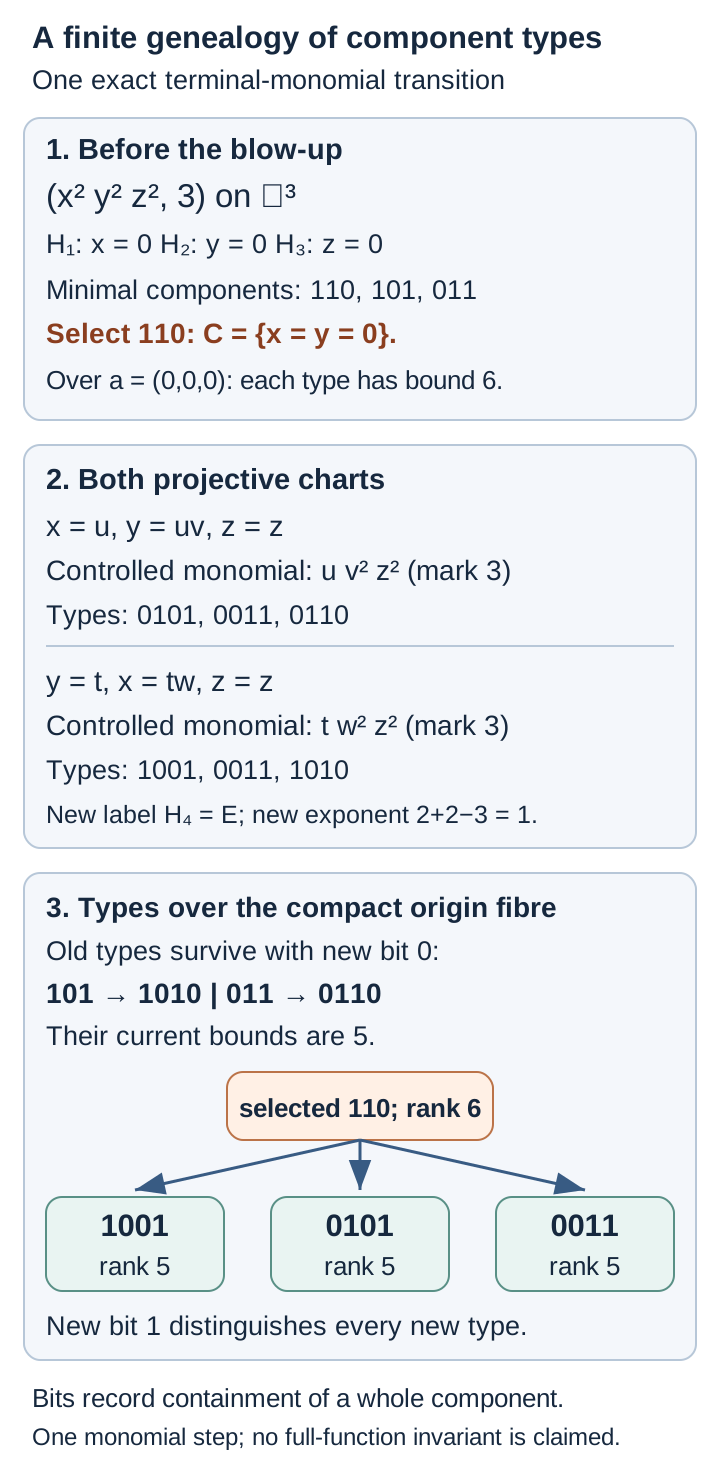
Over the original origin the old weight is . The new fibre is the exceptional projective line with ; each of the five displayed types meets a chart endpoint with incident weight . Thus its bound on that fibre is . The diagram illustrates the type transformation and rank estimate (TN12a)–(TN14) in one terminal-monomial step; it does not identify this marked example with the full recursive invariant of the unmarked function. The general mechanism is compared with Bierstone–Milman’s 25 November 1996 author manuscript, pp.39–40; the displayed example and figure are independently calculated here. Reproducible Python source enumerates the minimal subsets and checks the exact chart types.
The resulting local resolution and the compact-local conclusion
We have proved that the construction stops after finitely many steps. At that stage the maximum on the compact fibre is zero. Apply (TN10) once more to the open unit locus. There are only finitely many previously chosen base neighborhoods, so the final one is an actual open neighborhood . Restrict every stage to . This gives a finite composite of proper analytic blowings-up with closed smooth permissible centres, ending with a unit weak ideal. Each restricted nonempty centre is still the canonical maximum centre: its word and label vector were upper bounds on the larger domain and were attained on the fibre, which all restrictions preserve. More generally, the restriction theorem (CC8)–(CC10) gives this conclusion and the correct history after deletion of genuinely empty-centre steps. Nonempty Cartier steps are never deleted.
The whole-function ledger now writes every pulled-back local generator as a unit times an integral monomial in a simple-normal-crossing divisor. Its support is precisely the zero set of the pulled-back function. The composite is surjective and proper, and the protected-complement lemma makes it an analytic isomorphism above the complement of the original critical-zero set . This set is intrinsic to a locally principal ideal: replacing a generator by a unit multiple multiplies its differential at a zero by that same unit. These properties follow from the established ledger and blow-up lemmas, not from merely resolving the reduced zero set.
Every compact subset of the base is covered by finitely many neighborhoods constructed this way. Each carries an actual finite canonical terminal tower. Their restrictions match by (CC11)–(CC12). This is the compact-local finiteness input for the subsequent proper analytic assembly. It does not assert a finite global blow-up sequence on an arbitrary noncompact base. The assembly uses these finite local maps and their canonical comparisons; it needs no additional termination claim across an infinite global tower.
The proof has covered finite and infinite terminal values, prefix drops and rebirth, residual normalization, old-divisor history, identity maps coming from Cartier centres, and the boundary of shrinking working domains. The finite-chart bounds are taken only near compact fibres of already constructed proper maps. No finite-type replacement of the analytic problem, global Noetherian topology of an open chart, or unproved extension across a working-domain boundary enters the argument.
From finite local towers to the global function resolution
We explain the passage from the finite local algorithm to the full real analytic statement. The relevant inputs are the preceding canonical-centre and termination results: around every base point there is a finite terminal tower, its centres are the full selected components of the maximum stratum, and the same centre rule is used after restriction to an open subset. Empty restricted steps are omitted. The argument must compare independently run finite towers before applying the earlier gluing lemma.
The corresponding analytic passage is treated in Bierstone–Milman, Canonical desingularization in characteristic zero, author manuscript of 25 November 1996, Theorems 13.2–13.3, pp.66–67. The construction below retains the ambient manifold and the full principal ideal throughout.
The independent-tower comparison has already constructed analytic comparison maps on full overlaps by matching every nonempty restricted centre. It also proves their compatibility with restriction and the cocycle identity. We use those maps here.
A finite tower over a neighborhood of a compact set
Suppose finitely many open sets carry finite terminal runs. Their union also carries a finite run. This is useful when a compact set is covered by finitely many of the local neighborhoods obtained in the termination theorem.
Before comparing component refinements, embed each patch’s incidence vector into the current global chronological label positions, padding labels absent from that patch with zero. This common label list is retained throughout the merge. At the start, each nonterminal local run has a greatest extended invariant value: that is the value of its prescribed first centre. Take the largest of these finitely many values. On a patch with smaller local maximum, the global centre is empty. On a patch with that largest value, use its prescribed first centre. These descriptions agree on overlaps by the common invariant and centre rule. Hence they give a smooth closed analytic centre in , with normal crossings with the total divisor. Its blow-up restricts to the prescribed first step on the patches it meets, and to an isomorphism on the other patches.
Maintain the chronological order of global exceptional labels. A label born on a step disjoint from a patch is absent there, so inserting its zero incidence coordinate does not change that patch’s next selected component. The preceding overlap comparison therefore continues to identify each patch with the unconsumed suffix of its given local run.
Each global step consumes at least one local step, and never adds a step to a local run. If the local runs have lengths , the merged run has at most
nonempty steps. At its endpoint all local weak ideals are units, so the global weak ideal is a unit. This proves a finite tower over the union without imposing a bound on the invariant throughout a noncompact manifold. Any compact set has such a neighborhood, by a finite subcover of the local termination neighborhoods.
The proper map and the protected complement
Take a countable locally finite cover of by relatively compact open sets, each contained in a neighborhood with a finite terminal run. Such a refinement is supplied by the nested-ball construction later in this lesson. Restrict the runs to those sets. Every resulting terminal map is proper and surjective, by the projective-incidence and finite-composition proof for the supplied tower. The overlap argument above supplies its full analytic comparison maps.
Put . At an order-one point with no old divisor the full-component centre rule is exactly the smooth weak-zero hypersurface, as calculated in the protected-complement lemma. Thus condition (R) holds. That lemma shows that every local terminal map is an isomorphism over the complement of .
This unchanged locus has dense inverse image. The original zero set has empty interior, because is not identically zero on any connected component. In every blow-up chart the pulled-back function is a nonzero analytic function: the total-transform formula gives a nonzero weak generator times a unit and integral coordinate powers. Its nonzero locus is dense by the analytic identity theorem, and is contained in the inverse image of .
All hypotheses of the proper gluing lemma now hold. The resulting manifold is Hausdorff and second countable, and the glued analytic map is proper, surjective and an analytic isomorphism over . The finite-cover argument in that lemma proves properness on every compact subset of ; it does not require one finite tower on all of .
The terminal weak ideal is a unit on each local model. Hence the total-transform formula gives
with a nonvanishing analytic unit. At a point of , at least one exponent is positive. The unit-normalization lemma absorbs the positive magnitude of into that coordinate, preserving all crossing hyperplanes. Its sign is constant after shrinking. Thus
in analytic coordinates near that point. This is the function-resolution statement in item 5, with the entire function and its multiplicities retained. Dimension zero uses the identity map: the hypothesis on connected components makes a unit there.
Exercise: why the number of global steps need not be finite
Let be the disjoint union of countably many copies , , and define . Show that is a second-countable real analytic manifold and that each compact subset meets only finitely many of its components. Explain why no single finite sequence of blow-ups with closed smooth centres of positive codimension can make these functions normal crossing everywhere, although finite resolution in neighborhoods of each compact set is compatible with a global proper map.
Solution. Countably many countable Euclidean bases give a countable basis for the disjoint union. Its component charts supply its real analytic structure. The open components cover any compact subset; a finite subcover shows that only finitely many components are met.
At the origin of , the germ is not a coordinate monomial. Its zero curve is singular and has a single tangent line, the -axis: all of its nonzero points have , and on approach to zero. If it were a smooth embedded curve there, its nonzero tangent in the -direction and the inverse-function theorem would give points of both signs of , a contradiction. Blowing up that point, in the chart following this line, gives
For , the strict weak curve at the chart origin is again singular, of the same form with replaced by . Inductively, after point blow-ups following this branch, its equation is , still singular. A total coordinate monomial cannot have such a singular strict branch: its branches outside exceptional components are smooth coordinate hypersurfaces.
On a surface, a positive-codimension smooth centre through that point is either the point itself or a smooth curve. A curve is a Cartier centre and its blow-up is an isomorphism, so it cannot remove the singularity. Centres missing the point likewise have no effect near it. At least point blow-ups along this chain are therefore necessary, regardless of additional steps elsewhere. Since is unbounded, no finite global smooth-centre tower suffices. Every compact set meets only finitely many , however, so this does not contradict compact-local finiteness or the glued proper resolution map. Additional steps needed to make a final smooth branch transverse to the exceptional divisor only strengthen the absence of a uniform global bound.
From resolved signs to compact analytic images
We now prove the equivalence used in (1), the set and map assertions in item 1, and the compact closed-set case of item 4. The argument uses the function resolution just proved and the earlier finite-cell and complement theorems, bounded-chart comparison, and strict frontier decrease, (D12). None of these steps uses an intrinsic analytic regular-locus theorem or a uniformization theorem as an input.
For this section write for the class defined locally by projections of relatively compact semianalytic sets with compact closure in their analytic domains. Write for the class defined by (1). The local comparison near the beginning of this lesson, followed by the earlier bounded-chart comparison, already proves . The converse requires compact parametrizations of closed sets. We construct those first.
Resolving a finite sign formula simultaneously
Factor lemma. Suppose analytic germs at the origin satisfy
Then each is an analytic unit times a monomial in the same coordinates.
Proof. The convergent real power-series ring is a domain: the lowest nonzero homogeneous parts of two nonzero series have nonzero product. The quotient by is another such domain. Hence divides a product only if it divides a factor. The largest exponent of dividing a nonzero analytic germ is finite, and division by that power leaves a convergent series. The exponent for a product is the sum of those exponents: after extracting the powers, reduce modulo and use its domain property.
Extract from every its powers of each coordinate. Extracting a power of a different coordinate does not change the remaining divisibility by , again by reduction modulo . Equation (U1) then says that the product of the residual factors is the unit . Each residual factor is a unit: its inverse is the product of all the others divided by . This proves the assertion without importing unique factorization of arbitrary analytic germs.
Consequently, resolve the product of the finitely many nonzero analytic functions in a sign formula. Near a point above its zero set, (LG2), or the ordinary implicit-function coordinate at a regular zero point outside the protected centre, gives (U1). Above a point where the product is nonzero, every factor is already a unit. On a sufficiently small connected coordinate box every residual unit has constant sign. Each equality or inequality in the pulled-back formula therefore depends only on whether each coordinate is positive, negative or zero. The set described by the formula is a union of coordinate sign strata. Identically zero functions cause no difficulty: evaluate their sign predicates first and discard them before forming the product; if none remain, use the identity map.
A compact source for a semianalytic closure
Compact sign theorem. Let be a relatively compact semianalytic subset of a real analytic manifold, with closure contained in its analytic domain. Then is the image of a compact real analytic manifold under an analytic map.
Proof. Cover by finitely many closed coordinate boxes , whose interiors cover it and whose closures lie in connected coordinate neighborhoods on which one finite analytic sign formula defines . Put . The box inequalities join that sign formula. Every point of belongs to the interior of some , so limits of points of show that
It suffices to treat one . Resolve the product of its nonzero defining functions on , as above. This gives a proper surjective analytic map , with the pulled-back sign formula a union of coordinate sign strata on suitable charts of . Define
This is a closed subset of ; it is compact because is compact and is proper. Its image is exactly
One inclusion follows from continuity. For the other, if tends to , choose using surjectivity. The set formed by this convergent sequence and its limit is compact. Properness gives a convergent subsequence of the , with limit and . Analytic manifolds are metrizable, so sequential compactness suffices here. It is essential to use the closure in (U3); the full inverse image can contain exceptional directions not approached from .
At each point of , take a monomial chart centered at that point and a smaller closed coordinate box centered at zero, contained in the chart. Finitely many such boxes cover by their interiors. In the larger open chart, closure of the finite union of selected sign strata is the union of their closed coordinate quadrants. Restricting those quadrants to the smaller box therefore covers exactly the part of in that box. Each resulting piece is a product of intervals of the form , , or the singleton . Coordinates absent from the formula may instead use , or its two half-intervals.
Each interval has an analytic parametrization by the compact circle :
for the positive, negative and two-sided intervals respectively; use the constant map for a singleton. Products give analytic surjections from tori onto every selected quadrant box. Compose with the analytic inverse chart and with . The images stay inside and cover it. A finite disjoint union gives the required compact source for , and (U2) gives one for . If source pieces have different dimensions, add unused circle factors to reach their finite maximum; the images are unchanged. Dimension zero uses a point, and the empty set uses the empty manifold.
Compact uniformization for the projection-defined class
Compact uniformization theorem. Every compact closed -subset of a real analytic manifold is the image of a compact finite-dimensional real analytic manifold under an analytic map to . In particular the map is proper.
Proof. Near each point of , choose a presentation , with a relatively compact semianalytic witness and compact closure in its analytic domain. Choose a closed base coordinate box , with the point in its interior. Restrict the witness to . This remains relatively compact semianalytic, and
For the middle equality, continuity gives one inclusion, and compactness of makes its image closed and supplies the other. The last equality uses that is closed. Thus no point outside the desired trace is introduced by closing the witness.
Apply the compact sign theorem to , then compose its parametrization with and the target chart inverse. This gives a compact analytic source with image exactly . Finitely many such boxes have interiors covering . Take their finite disjoint union, padding with unused circles if necessary to make the source dimension constant. A continuous map from a compact space to the Hausdorff manifold is proper.
The two definitions agree
Fix a -set and an ambient point . Restrict to a sufficiently small open coordinate box about , with compact closure inside the witness neighborhood. In coordinates its trace is globally subanalytic by the earlier bounded-chart comparison. Its closure is compact in the target chart. Recursively put
All these sets are globally subanalytic by the proved Boolean and closure calculus; all are compact. The strict frontier theorem gives whenever . With the empty-set dimension equal to , the sequence therefore reaches the empty set after finitely many steps. Also , and two successive substitutions in (U7) give
Consequently is the finite union of the alternating differences
where all sufficiently late are empty. Each compact closed is a -set also when viewed in , because its closure stays inside the chart. Compact uniformization represents it as one compact-manifold image in . Equation (U9) is exactly the form (1) near . This proves , and hence the equivalence of the two definitions.
The dimension used in this terminating argument is the finite-cell dimension already proved in the preparation lesson. It does not use the separate intrinsic regular-locus theorem in item 2.
The local calculus with the precise properness hypothesis
We can now transfer the proved bounded global calculus to the class in (1). Given finitely many local subanalytic sets near an ambient point, choose one smaller closed chart box inside all their witness neighborhoods. Their traces are globally subanalytic. Finite unions, intersections, differences, closures and interiors are globally subanalytic there, and on the interior of the box their closures and interiors agree with the corresponding local operations. Restriction and the definition equivalence prove the asserted local set calculus.
Connected components. On such a bounded chart trace there are finitely many connected components, each globally subanalytic by the finite-cell theorem. Every global connected component of meeting the interior chart contains one of these whole local components: a connected subset meeting a connected component is contained in it. Thus only finitely many global components meet that neighborhood. The intersection of any particular global component with the neighborhood is a union of some of the finitely many local components, restricted back to the neighborhood, so is subanalytic. This proves component subanalyticity and local finiteness at every ambient point, including points outside .
Analytic inverse images. For an analytic , choose a target chart inside the target set’s witness neighborhood and a smaller bounded region around the image of the point under consideration. By continuity choose a small closed source chart box whose image lies in that region. On that box the graph of is globally semianalytic: its analytic coordinate functions extend to a neighborhood of the compact box, and the box inequalities bound the graph. Intersect it with the target set’s bounded subanalytic trace, then project to the source coordinates. This is globally subanalytic by graph calculus. Restricting to the source box’s interior proves that is locally subanalytic. No properness hypothesis is needed for this direction.
Images proper on the selected closure. Let be subanalytic and suppose only that is proper. Around a target point choose a compact coordinate box , with that point in its interior. Then
is compact. Cover it by finitely many closed source chart boxes whose interiors cover , each lying in a bounded witness chart for and in the inverse image of the target coordinate chart. Graph intersection and projection on these compact boxes show that each is subanalytic in target coordinates. More explicitly, intersect the compact analytic graph with the globally subanalytic source trace , and project. Every preimage in of a point in belongs to , so
This proves the image assertion with exactly its stated closure-properness hypothesis. The map need not be proper on all of , and the argument does not replace by the larger .
These results prove item 1 and compact closed-set uniformization. Local compact parametrizations alone would not control the dimensions of the sources over a noncompact base. The rank-minor reduction and locally finite assembly below supply that control and complete item 4. A finite analytic partition does not by itself identify every intrinsic regular point; the analytic-descent argument establishes that stronger assertion.
Exercises on the compact construction
Exercise U1 (intermediate: the exceptional fibre is too large). In the real blow-up of the origin of , consider the chart and the positive horizontal ray . Compare and in this chart.
Solution. The inverse image of in this chart is . Its closure is , meeting the exceptional line only at . The inverse image of contains that set and the whole line , because every point of the line maps to the origin. Globally the latter inverse image contains the whole exceptional projective line, whereas the former closure meets it only in the horizontal direction. Formula (U3) retains precisely the directions actually approached by the chosen set.
Exercise U2 (intermediate: an alternating boundary expansion). Let . Compute the nonempty sets in (U7) and verify (U9).
Solution. Put and . Then , , , , and . The dimensions of the nonempty are , decreasing strictly. The alternating formula gives , as required. Using only would incorrectly lose the selected boundary point.
Dimension-controlled proper uniformization
Compact source maps carry more parameters than their images need. A height function detects a smaller analytic subset meeting every compact fibre. Resolving its rank-minor equation reduces the source dimension without losing any image points. Repetition gives one dimension bound for all local pieces; a locally finite target cover then makes their disjoint union proper.
The classical dimension-preserving uniformization theorem is proved in Bierstone and Milman, Semianalytic and subanalytic sets, Proposition 3.12 and Theorem 5.1, printed pp. 19–20 and 30–32. The argument below uses the compact torus parametrizations and the function resolution already established in this lesson.
Reducing the dimension of a compact analytic source
The compact construction above gives finite unions of torus sources, but their dimensions initially depend on the semianalytic witnesses. We now reduce those dimensions while preserving each image exactly. The inputs are the proved proper function resolution (LG2), the analytic constant-rank and inverse-function theorems, and compactness. The rank reduction itself uses no subanalytic regular-locus theorem or analytic-set uniformization.
Write The fields form a global analytic tangent frame. We take to be one point. Both and are globally defined analytic functions on the torus.
One-step reduction lemma. Let be analytic, let , and suppose . There are finitely many analytic maps such that Every replacement map is a composition with . In particular its differential rank is at most .
Proof. Choose of rank , and a nonzero vector . The differential of the displayed inclusion is injective. Consequently at least one of its coordinate functions, denoted by , satisfies . Thus is not in the row space of , and has rank .
Form the global analytic -by- matrix whose rows are the derivatives of along the frame (N1). Define There are enough rows and columns because and . The sum is finite, and it is positive at . Moreover, over the real numbers, if and only if . Since , the torus is connected; the nonzero value at verifies the nonidentical-vanishing hypothesis of function resolution on every connected component of this source.
We claim that Fix . The fibre is a nonempty closed subset of the compact torus. Let minimize on it. If , adjoining one row gives rank at most , so . If , a nonzero -minor stays nonzero near , while the global maximality of gives the opposite rank bound. Thus has constant rank there. The constant-rank theorem makes its local fibre a smooth analytic manifold with tangent space . The minimum of on that fibre implies . Hence adjoining does not increase rank, and again . For , this latter argument simply uses a locally constant , whose local fibre is the whole source neighborhood. Every fibre meets , proving (N3); the reverse inclusion was automatic.
At every zero of , all minors in (N2) vanish. Differentiating their sum of squares therefore gives there. Thus , and the existing resolution theorem’s singular-zero conclusion covers every point of the inverse image of .
Apply the proved proper function resolution to the single nonzero analytic function . It gives a proper surjective analytic map , with an -dimensional analytic manifold, and local coordinates in which is a nonvanishing unit times a monomial. The source dimension is unchanged by the blow-up charts and their analytic gluing in that theorem. Because is compact, properness makes compact. Put . Then is compact and , by surjectivity and the equality defining this inverse image.
At each point of , choose a monomial coordinate neighborhood and a smaller centered closed coordinate box , with all , whose closure stays inside that neighborhood. The interiors of finitely many such boxes cover . In any one of these charts, if , then the part of in the box is exactly the union of for those with . There is at least one such index at the chosen centre of the chart.
Each of these closed hyperplane boxes is the analytic image of : give its circle factors the indices , and set The coordinate functions are surjective, so the image is the entire hyperplane box. Composing (N4) with the analytic inverse chart gives an analytic map into . This is analytic also at points mapping to the edges of the box: the inverse chart is defined on a neighborhood of the whole closed box. Its image lies in , not merely in an approximation or closure of . For , (N4) is the map from one point to the zero coordinate.
Compose these finitely many maps with , calling the resulting maps . Their images lie in and cover . Therefore (N3) yields The chain rule gives . This proves the lemma. Notice that singular fibres were retained in the lower-rank case, and exceptional components were retained in . Neither was discarded.
Finite rank-bound reduction. If is a nonnegative integer, then the image of an analytic is a finite union of analytic images of . These maps can all be written as , with .
If , compose with the projection , which preserves the image. If , do nothing. If , apply the one-step lemma. Each new map has rank at most by the chain rule, so the same argument applies whenever its source dimension still exceeds . The dimension drops by exactly one at every replacement, and each replacement has finitely many outputs. Induction on therefore ends after at most levels with finitely many maps and gives All compositions are analytic on their entire compact source. The number of branches need not have a uniform bound across different initial compact problems; the conclusion of each individual problem is finite. Taking already gives the uniform ambient-dimension bound required for the noncompact construction.
The same conclusion holds for an analytic map from an arbitrary nonempty compact analytic manifold into a finite-dimensional analytic manifold , with . To see this without an embedding theorem, cover by the interiors of finitely many closed coordinate boxes, each lying inside a source chart and mapping into one target chart. Each box is an analytic image of a torus of its dimension by the product version of (N4), now with no coordinate fixed to zero. The inverse source chart is defined on a neighborhood of the closed box. Composing with gives finitely many torus maps whose images cover exactly. Their ranks are at most . Apply (N6) in their target charts, padding smaller initial torus dimensions if necessary, and compose back with the target chart inverse. The result is a finite union of compact -tori mapping analytically into , with image exactly . Empty sources are omitted.
Comparing the rank bound with cell dimension
The sharper bound uses the already proved finite-cell dimension, not an intrinsic regular-locus assertion. The relevant provider is Why cell dimension is intrinsic: (D4) gives inclusion monotonicity, and the paragraph following it identifies the cell dimension of a definable differentiable manifold with its manifold dimension. The same provider proves invariance under bounded analytic changes of coordinates. Its established attribution and CC BY 4.0 component notice remain in force.
Here is the exact application, including the boundedness needed for that provider. Suppose an analytic has image in a locally subanalytic set , and let bound the cell dimensions of the bounded coordinate traces of . At a point where has rank , choose an invertible -by- derivative minor in source and target analytic coordinates. Fix the remaining source coordinates at their values at . The analytic inverse-function theorem on this transverse -dimensional slice parametrizes a part of its image as a graph over the corresponding target coordinates. Choose a nonempty open box in those coordinates whose compact closure stays inside the graph domain and whose graph stays in a target chart trace used to define . The graph functions are analytic on a neighborhood of that closed box. Their restricted graph is therefore globally subanalytic by the proved bounded-chart comparison; it is an embedded analytic -manifold and is contained in .
The manifold-dimension statement gives this graph cell dimension , and inclusion monotonicity bounds it by the dimension of the chosen trace of , hence by . Rank zero satisfies the same inequality whenever is nonempty. Thus No analyticity of the intrinsic regular locus of is used: the graph is constructed directly inside the image of .
For a nonempty in an -manifold, its locally defined cell dimension is an integer with . It is well defined by the proved chart invariance and finite-union rule, and the maximum exists because the possible dimensions lie in this finite set. Combining (N6)–(N7), every compact parametrization supplied above can be replaced by a finite union of compact analytic sources of dimension at most , with exactly the same image. Multiplying a source of dimension by the unused compact factor makes its dimension exactly , preserves its image and preserves compactness. Alternatively apply (N6) with directly. These are the dimension-controlled compact sources needed for the locally finite proper assembly. The empty set uses the empty manifold, without assigning it a negative manifold dimension.
Example for the mechanism. On , take and . Then , , and . Its zero set is the union of four coordinate circles, two given by and two by . On every fibre of , the minimum of occurs on the circle , which still maps onto the whole interval . The circles retain the lower-rank fibres over the endpoints. This explicit example explains the equality of images; the general proof uses the full zero set and its compact monomial charts.
A locally finite assembly with a fixed source dimension
Proper uniformization. Let be a nonempty closed subanalytic subset of a finite-dimensional real analytic manifold , Hausdorff and countable at infinity. Let be its finite-cell dimension. There is a Hausdorff, second-countable real analytic manifold , of pure dimension , and a proper analytic map
If is compact, can be compact. The empty set is represented by the empty manifold. Properness is relative to the stated ambient manifold .
Proof. The elementary locally finite compact chart construction, (F2)–(F4), gives a countable family of closed coordinate boxes , each contained in an analytic coordinate neighborhood , with locally finite family and with interiors covering . The boxes can be chosen subordinate to the witness neighborhoods used in the projection definition of . This construction uses only an exhaustion by nested compact sets and finite covers of its compact bands. It does not use uniformization or an analytic partition of unity.
Since is closed in , each is compact and subanalytic. The compact construction above represents as a finite union of analytic images of tori. Every such image lies in , hence entirely in the target chart . Apply the preceding dimension-reduction lemma in that chart. It produces finitely many maps
An empty contributes no maps. For , add unused circle factors and let ignore them. This preserves its analyticity, compactness and image. Define as the disjoint union of these copies of , and define componentwise by the corresponding maps.
There are countably many components, each a Hausdorff second-countable analytic -manifold. Their disjoint union is Hausdorff and second countable: unite one countable basis from each component. It has the same finite dimension everywhere. Componentwise charts and transition maps make analytic. The cover by the interiors of and (N9) prove .
To check properness, let be compact. Local finiteness and a finite subcover of show that only finitely many meet . Thus lies in finitely many of the compact source tori. It is closed there, because is closed in the Hausdorff space and is continuous. Consequently is compact. This proves properness without requiring the images of different source components to be disjoint.
When is compact, finitely many of the chosen interior boxes cover it. Using just those boxes and their finitely many tori gives a compact , and the same image equality. The dimension-zero case uses , a point, and the same locally finite argument.
The dimension in (N8) also equals the supremum of the dimensions of intrinsic analytic regular points, as used in item 2. Here only that numerical equality is needed; it does not assert subanalyticity of the entire regular locus. To prove it, choose a bounded open coordinate box , with closure inside a witness neighborhood, such that . Take a finite analytic cell decomposition of containing a cell of dimension . Every point of this trace lies in the open set , so its cells describe near that point. For every other cell , its intersection with is empty, and
The finite-cell dimension and strict-frontier theorems imply that these finitely many intersections cannot cover . Choose outside every . A small ambient neighborhood meets no other cell. As an embedded analytic submanifold, is closed in a sufficiently small neighborhood of , and there . Thus is an intrinsic regular point of dimension . Conversely, a regular -dimensional manifold piece contained in has by manifold dimension and monotonicity. This gives the claimed numerical equality. The analytic-descent proof below establishes definability of the entire intrinsic regular locus.
A compact fibre meets the minimizing circle
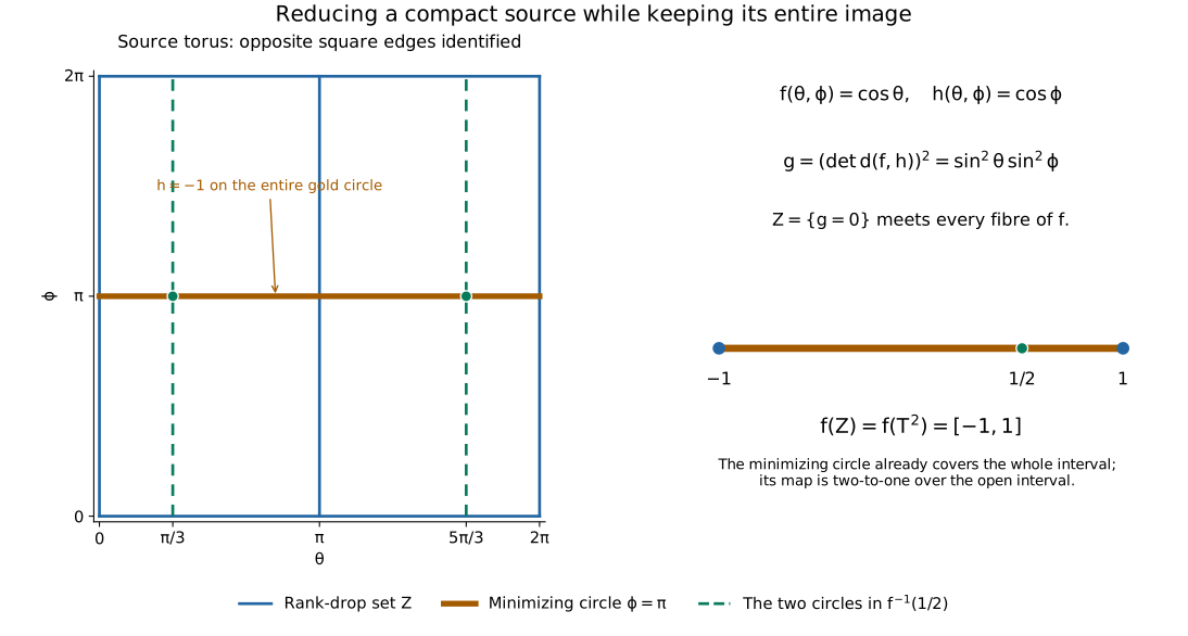
Figure. Write each circle as or . For and , the squared determinant is . The blue grid is ; opposite edges of the square are identified. The gold circle is part of and minimizes on every fibre. The two dashed circles form , and their two intersections with the gold circle map to the indicated green point. The image is preserved even though the minimizing circle maps two-to-one over . This is the explicit model of the rank-minor and fibre-extremum argument, not an injective parametrization. Original programme diagram, GPT-6 Astra (OpenAI), Ultra, CC0. Full-size diagram · Reproducible Python source.
Exercises on dimension control and properness
Exercise N1 (intermediate: retaining singular fibres). In the displayed torus model, compute the set , verify that it meets the fibres over and , and exhibit a one-dimensional compact analytic source with the same image as the original two-dimensional torus.
Solution. The matrix of in the angular frame is diagonal with entries and . Hence is the union of the circles , , , and , with angles interpreted modulo . The endpoint fibres are the entire first two circles, so they are retained, not discarded as exceptional. The circle maps by onto . It is a compact one-dimensional analytic source with the full image. An interior fibre has two points on this selected circle; an endpoint fibre has one. No injectivity or preservation of the original fibres is part of uniformization.
Exercise N2 (intermediate: componentwise properness is insufficient). Let be a countable disjoint union of points and map every point to . Explain why every component map is proper, but the combined map is not. Also distinguish properness of the identity of from properness of its inclusion into .
Solution. Each point is compact, so its map is proper. The inverse image of the compact set under the combined map is the infinite discrete space ; its cover by singleton open sets has no finite subcover. The image supports are not a locally finite family, which is exactly the hypothesis used in the proof of (N8). The identity of is proper because inverse images of compact subsets are those same subsets. Its inclusion into is not proper: the inverse image of is all of , which is not compact. Therefore the ambient target in a proper uniformization statement must be retained.
Detecting the entire analytic regular locus
A cell partition supplies many analytic manifold points. Recognizing every such point, including points crossed by an unnecessary cell boundary, requires a test independent of the partition. We will use analyticity of squared distance to a closed set, after proving that a continuous subanalytic function has a subanalytic analyticity locus.
The graphic-point mechanism comes from Malgrange, as used by Bierstone and Milman in Semianalytic and subanalytic sets, §7, printed pp. 37–41, especially Proposition 7.4 and Theorems 7.5–7.10. The proof below expands the local convergence and compact descent arguments. It uses compact uniformization and the compact rank reduction (N6); the locally finite noncompact uniformization assembly and a finite-smoothness version of Tamm’s theorem are not inputs.
The complex analytic providers are the proved contour preparation and division theorem, unique factorization of holomorphic germs, and finite branches with connected dense smooth cores. These concern complex analytic sets and do not assume the real subanalytic regular-locus statement being proved.
Convergence at a critical source point
First, if are convergent complex power series, , and for a formal series , then converges. Make regular in one variable and write , with distinguished. Divide analytically by . Uniqueness of formal division by the same distinguished polynomial makes the analytic remainder zero and identifies the analytic quotient with . Formal division follows coefficient by coefficient in the other variables: modulo their successive powers, division by the leading power of the distinguished variable determines quotient and remainder.
Lemma. Let be holomorphic of generic rank . If and converges, then converges.
Proof. The case is constant and immediate. Choose a nonzero -rowed Jacobian minor , after reordering source coordinates. On , differentiation with respect to the first coordinates in has the form with holomorphic cofactors . Set . Its numerator is holomorphic on one fixed sufficiently small source neighborhood and its denominator is a power of . Formal differentiation gives Here the equality is first in the fraction field of formal series; its right side lies in the formal series ring. The divisibility observation makes every holomorphic as a germ at zero.
Moreover as a germ. The meromorphic identity extends to the fixed connected source neighborhood. Thus, wherever , is independent of the unused local coordinates, and is a holomorphic function of alone. The commute there, so the derivative order used to define is immaterial.
We now obtain one neighborhood for all . Make an additional linear source change so is regular in a variable , and prepare The already defined meromorphic operators are simply transported under this change. Retain the original complementary functions as fixed linear functions in the new coordinates; they are not replaced by arbitrary new coordinate functions. The map remains a local coordinate system wherever . Choose a circle and a connected smaller -polydisc such that on the circle and all roots of lie strictly inside it. The original holomorphic functions and the unit are defined on a neighborhood of the closed cylinder.
For every , write , with holomorphic on that fixed neighborhood. The contour division formula divides by the monic polynomial on the same cylinder, producing a polynomial remainder whose coefficients are holomorphic throughout the fixed -polydisc. At the origin this remainder vanishes as a germ: was holomorphic there, so uniqueness of Weierstrass division applies. The coefficient identity theorem makes it zero on the whole connected -polydisc. Consequently every is holomorphic on the common interior cylinder. No bound on is required; the same circle avoids the zeros of all denominators.
On the compact circle , use the local inverse of to form At each point of , this is holomorphic on a product of a source neighborhood and a positive target polydisc. Shrink both so it is bounded on their closures. The source neighborhoods have a finite subcover of . Taking the largest of their bounds and the smallest target radius gives constants such that Cauchy’s estimate yields for every multi-index. The equality uses the retained complementary functions, so these are exactly the transported operators . No gluing of the functions is needed for the estimate.
The common-cylinder holomorphic extension and Cauchy’s formula in , with , give Thus the coefficients of satisfy . The product of the geometric series proves absolute convergence when every . This proves convergence at the original, possibly critical, source point.
The local obstruction to an analytic graph
Let and be analytic, with . Assume that has generic rank on every component of , and that A point is graphic if an analytic germ at satisfies . Such an is unique. Regular points of occur arbitrarily near , and their images contain open target sets. Equality of two pullbacks therefore forces equality of the two target germs by the analytic identity theorem.
Condition (IR1) is necessary: , has no graphic points, although has full rank. For a parametrization of a function’s graph, (IR1) is automatic, since is constant on each local fibre at a submersion point.
One-point obstruction lemma. The non-graphic set is closed real analytic and lies in the critical set of .
Proof. Complexify small real coordinate neighborhoods. The differential identities in (IR1) extend holomorphically. Choose a nonzero Jacobian minor , and form the meromorphic functions used in the convergence lemma. Off , condition (IR1) makes locally a function of , and the are its descended derivatives. Their denominators are powers of .
Suppose all are holomorphic at . Define For every , the Taylor-composition identities through degree hold at regular points. They are holomorphic identities involving only finitely many , so extend to . Hence The convergence lemma makes convergent, so is graphic. Conversely, a graphic germ gives , so every is holomorphic. Thus is exactly the union of their pole loci.
This infinite union is analytic for a specific reason. Shrink to a fixed complex neighborhood where has finitely many irreducible hypersurface components. Each meromorphic function with denominator a power of has pole locus equal to a union of some of these components. Local unique factorization tests which denominator factors cancel. On the connected dense smooth core of an irreducible component, the identity theorem propagates such cancellation along the component; local factorization then extends it at its remaining points. A genuine uncancelled factor instead gives a pole along the entire component, because the holomorphic locus is open. Local unique factorization also excludes a pole supported only in smaller codimension. Therefore the union of all the pole loci is a union of a subset of the same finite list of components, hence analytic.
Conjugation preserves the construction. Denote its complex analytic pole set by . At a real point any complex descended germ equals its conjugate, since their pullbacks agree and descent is unique. Thus the real non-graphic set is exactly . Retain the constructed complex set, which can be larger than a minimal complexification of this real trace. Using any nonzero minor shows that every regular point of is graphic. These local sets agree because their defining property is intrinsic.
Comparing two points of a fibre
The fibre product is analytic. A pair is graphic if one germ works at both points. Write for the pairs that are not graphic.
Two-point obstruction lemma. The subset is closed analytic.
Proof. Work directly on complexifications of the two source charts and their common target chart, and use the complex pole sets constructed in the preceding proof. Write for the resulting holomorphic fibre product. A complex graphic pair stays graphic on a neighborhood, using the same representative , so its non-graphic set is closed. Put using the appropriate source chart in each factor. This analytic set is contained in . In particular, is formed from the actual complex pole loci, not from an arbitrary complexification of their possibly smaller real traces.
On , agreement of the two descended germs is locally constant. Near a pair, represent the two germs by holomorphic functions on one connected target ball. Either they agree identically, or their germs agree nowhere on that ball: germ equality would imply equality on an open set and then everywhere. Uniqueness of descent identifies these with the germs at all nearby pairs.
Take finite irreducible branch representatives of at the pair. A branch contained in is wholly bad. On every other branch, take a connected dense smooth core and delete . The complex branch and analytic-deletion results make this a connected dense set, on which the locally constant condition is either always good or always bad. In the bad case, closedness puts the whole branch in . In the good case, every point of the branch outside is good, since its neighborhood meets the dense good core and the condition is locally constant there. Hence, after a common shrinking, This is analytic. Connected cores are retained on their original larger representatives until the final shrinking; connectedness of an arbitrary smaller branch intersection is not assumed. Conjugation and uniqueness identify the real trace with , proving the claim.
Analyticity of a continuous subanalytic function
Analytic-locus theorem. If is continuous and subanalytic on an open subset of an analytic manifold, then is open and subanalytic.
Proof. Openness is part of the definition. In a coordinate chart, choose a closed box whose interior contains the point being considered and whose closure lies in . The graph of is compact, closed and subanalytic. Compact uniformization gives a compact analytic manifold and an analytic map
Discard components on which the generic rank of is less than . There are finitely many components, since is compact. For a discarded component , put . The compact rank reduction (N6) writes as a finite union of analytic images of . The image-dimension inequality (D5), applied to those compact torus maps in bounded charts, gives . Thus each discarded image has empty interior. The images of the retained components form a compact, hence closed, set containing the dense complement in of the discarded images. They therefore cover all of . The retained map still covers the graph, has generic rank on every component, and supplies (IR1).
The closed analytic set in the compact fibre product has compact subanalytic image under , by the already proved proper-image calculus. We claim If is analytic near , its germ works at every pair above .
Conversely, suppose there is no bad pair above . Diagonal pairs show that each individual point of the fibre is graphic. Fix in the fibre. Its pairs with all other points, and uniqueness of descent at , show that every descended germ is one common germ . Compactness of the fibre gives finitely many source neighborhoods covering it on which , after choosing a common representative and shrinking its target neighborhood. The compact set has closed image missing . A smaller target neighborhood thus has . Every point of has a preimage; there . Hence is analytic near , proving (IR6) and subanalyticity.
The test considers every pair of points of each fibre. Neither a bound on fibre components nor a dimension bound shared with parametrizations on other target charts is needed.
Squared distance recognizes an analytic submanifold
For a nonempty closed , put . At ,
Proof. If is analytic near , rotate coordinates so it is the graph , with , . The analytic normal-coordinate map has invertible derivative at zero. A nearest point to sufficiently close to zero lies in this graph, since its distance from zero is at most . Its displacement from is normal to the graph by stationarity of squared distance. The inverse-function theorem gives a unique such point , analytic in . Thus is analytic.
Conversely assume analytic near . Every first derivative of vanishes on , since and . Choose an analytic submanifold of smallest dimension containing the germ of at ; the ambient space is one candidate. If near , then there. Otherwise choose tending to , and nearest points . Both sequences tend to and eventually lie in . Pass to a subsequence with The tangent assertion follows by expressing as a differentiable graph and estimating the difference of two graph values by its derivative near .
On the segment from to , distance to equals distance to . One inequality uses ; the reverse follows by the triangle inequality measured from . Thus The function vanishes on and has nonzero derivative in the tangent direction at . Its zero hypersurface cuts transversely, producing a smaller-dimensional analytic submanifold still containing the germ of . This contradiction proves (IR7).
At a regular point of local dimension , the same normal coordinates give
Every intrinsic regular point, in each dimension
Let be subanalytic in an -dimensional analytic manifold. Work in a relatively compact chart and close a slightly larger bounded trace of to get a compact subanalytic set ; in a smaller region is the ambient closure of . The empty case is immediate.
The function is continuous and globally subanalytic in these coordinates. Its graph is given by the minimum of polynomial squared distance over the compact definable set ; the minimum and its equality condition are formulas with quantifiers over definable sets. Boolean and projection closure therefore give subanalyticity. The triangle inequality gives continuity. Equations (IR5)–(IR7) yield
On any smaller bounded working region, bounded-chart comparison makes the subanalytic open set definable. Its Hessian entries are subanalytic. Indeed, the graph of a derivative wherever it exists is expressed by the quantified condition for the difference-quotient limit. Boolean and projection closure give definability; apply this twice on the analytic open set. Rank is expressed by finitely many minors. Hence is subanalytic for every .
For a set that is not closed, the exact local identity is If agrees with a closed analytic submanifold on a neighborhood, so does its ambient closure, and missing points cannot approach the selected point. Conversely, outside the second closure in (IR10), and agree on a neighborhood. This proves the identity. The previously proved local calculus now makes every , their finite union , and subanalytic. Regularity is relatively open in , so its complement is relatively closed.
Regular points are dense in . In any sufficiently small bounded open chart meeting , choose a finite analytic cell partition of the trace and a cell of maximal dimension . For every other cell , The strict frontier theorem gives dimension less than for this intersection, since . These finitely many intersections cannot cover . At a point of outside all the other cell closures, the entire set agrees locally with . An embedded analytic cell is locally closed; shrinking the neighborhood makes it a closed analytic submanifold there. This is an intrinsic regular point. Every ambient neighborhood meeting consequently meets .
The same argument identifies cell dimension with the supremum of dimensions of regular germs. It produces a regular germ of maximal cell dimension, while a -dimensional regular germ cannot be covered by finitely many smaller-dimensional cells, by the cell-dimension volume argument. This proves all assertions of item 2, including every fixed-dimensional part. It does not identify regularity with membership in a chosen top stratum.
Exercise: separate graphic germs need not agree
Let be two disjoint circles , and define Their union parametrizes the compact graph of , . Show that every source point is graphic, while the target germ at zero is not analytic.
Solution. On the positive circle the descended germ is ; on the negative circle it is . The identities hold even where , so the one-point obstruction is empty. At zero a pair with one point from each circle cannot share one descended germ: uniqueness would require as germs. Thus the two-point obstruction has an image at zero. The one-sided derivatives of there are and . Equality of fibre values alone misses this disagreement of germs.
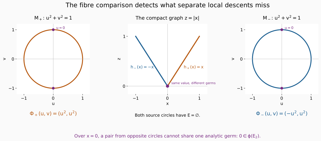
The two maps in the exercise are analytic on their full source circles. The purple points all lie over zero; a pair from opposite circles has the same function value but no common analytic germ. This is the distinction tested by (IR3)–(IR6). Full-size diagram · Reproducible Python source.
Compatible locally finite analytic partitions
The finite analytic cell theorem, its Boolean and projection calculus, and its bounded-chart comparison give the following manifold partition. The compact chart-ball refinement is proved below in Section 2 of the cutoff construction. These are the exact inputs; no analytic regular-locus theorem or uniformization theorem is needed for this partition.
Partition theorem. Let be a finite-dimensional Hausdorff second-countable real analytic manifold without boundary, and let be a locally finite family of locally subanalytic subsets. There is a countable locally finite partition of into connected locally subanalytic embedded analytic submanifolds compatible with every : each partition member is contained in or disjoint from each . Given finitely many analytic maps to real analytic manifolds, the partition can also make every restriction have constant rank.
Compact chart pieces and compatibility
The compact exhaustion and shell construction in the linked cutoff proof supplies a countable cover by open coordinate balls with compact closures contained in analytic charts; the family of these closures is locally finite. For instance, use the inner balls in that construction: their closures are contained in its locally finite outer compact balls. Each ball and its closure is locally semianalytic. In its chart it has a squared-norm inequality, and outside its compact closure it is empty on a neighborhood. The exhaustion sets need not be subanalytic; only the selected balls enter the partition.
For the map assertion apply this refinement to the open cover consisting of intersections of a source chart and inverse images of target charts for the finitely many . Thus each lies in one source chart, and every lies in one selected target chart. The source and target coordinate images of these compact sets are bounded. The maps in these coordinates are analytic on a neighborhood of .
Every compact set meets only finitely many members of a locally finite family. Indeed, cover the compact set by finitely many neighborhoods, each meeting finitely many family members; combine their finite lists. In particular meets only finitely many and finitely many nonempty .
Enumerate the balls and put
These sets are disjoint and cover , because each point has a first containing ball. For fixed the earlier union is finite; its trace near uses only the finitely many earlier closures that meet a sufficiently small neighborhood of . To justify that neighborhood, first take a finite cover of by neighborhoods meeting only finitely many closures, then discard the finitely many closures missing by shrinking around that compact set. Thus is a finite Boolean combination of locally semianalytic balls near . The local Boolean calculus also makes every relevant locally subanalytic there.
In the chosen source coordinates, these traces are bounded and locally subanalytic at every point of their ambient closures. Their closures lie inside the compact coordinate image of , strictly inside the source chart. Extension by the empty set therefore creates no chart-boundary obstruction. The proved bounded-chart comparison makes and all the finitely many relevant globally subanalytic in this Euclidean space.
Apply the finite analytic cell theorem compatibly with these sets, and keep just the cells in . Each kept cell is a connected embedded analytic submanifold. Its global subanalyticity gives local subanalyticity in the source chart, including at points of its closure; compact containment gives local emptiness outside that chart. It is therefore locally subanalytic in . It lies in or misses every , including those whose trace on is empty.
There are finitely many kept cells for each , and each is contained in . A neighborhood meeting only finitely many consequently meets only finitely many kept cells. They give a countable locally finite partition of . This proves the first assertion. It uses local finiteness of the compact closures; a merely countable atlas does not supply that conclusion.
Analytic coordinates on a cell
We spell out the cell coordinates needed for rank refinement. A cylindrical analytic cell of dimension has a coordinate projection which is a definable analytic diffeomorphism onto an open definable . Keep precisely its band coordinates and discard its graph coordinates.
This follows by induction through the cylindrical construction. For a graph over a cell with inverse parametrization , use ; the old free-coordinate domain remains open. For a band over that cell, the new free domain is
It is open because the endpoints are continuous, omitting the corresponding inequality for an infinite endpoint. Its inverse parametrization is . These maps and their inverses are analytic. Their graphs are definable by the graph, composition and projection calculus; hence the domains are definable too. In dimension zero use the single point . This proves the coordinate assertion, including the analytic embedding and its inverse, directly from the cell definition.
Definable derivatives and restriction ranks
Fix a kept cell , and write for this inverse parametrization. In the chosen target coordinates the maps are analytic and definable. To check the latter assertion, the coordinate graph of over is bounded and locally semianalytic at every point of its compact closure: its defining analytic equation is valid on a neighborhood of , and the closed coordinate ball supplies the domain condition. The bounded-chart comparison gives a globally subanalytic graph. Restriction to and composition with preserve definability.
For a scalar analytic definable , the derivative graph, with , is described by
Function values here can be written using extra real variables in the graph of ; division by is a polynomial graph condition. The formula uses finitely many real quantifiers. Existential quantification is projection, and universal quantification is complement of an existentially quantified complement. Thus the established Boolean and projection calculus makes this derivative graph definable. Openness of supplies a nontrivial interval of allowed at every , so the limit condition specifies the derivative uniquely. Applying this to every scalar coordinate gives definable differential matrices for all .
All rank sets are consequently definable: rank means that every -minor vanishes and, when , some -minor is nonzero. Rank zero means every matrix entry vanishes. Include all finitely many rank sets for the finitely many maps in a finite analytic cell decomposition of .
Every resulting -dimensional cell is open in . Indeed, a full-dimensional cylindrical cell has only band steps, and (P2) proves openness at every such step. Therefore is open in ; its tangent space is that of , and every has the constant rank selected on . Retain these members as finished.
On a smaller cell , the old differential rank is insufficient: restricting a rank-one map to one of its level curves can give rank zero. Take the cell’s own free-coordinate parametrization , and repeat the rank calculation for all . These are still definable analytic maps on an open definable domain. Their images under are connected embedded analytic submanifolds and definable in the original source chart. Repeat the same finite refinement and finish its full-dimensional members.
An unfinished branch now has strictly smaller dimension. Induction on terminates: dimension zero has rank zero for every map, and each positive-dimensional step finishes its full-dimensional cells and passes only finitely many smaller cells to already established lower-dimensional cases. The final refinement of each original is finite. Its members remain inside , so refining the finitely many cells for each preserves countability, local finiteness and compatibility with all . This proves simultaneous constant rank on every final member.
If is compact, this locally finite partition is finite by the compactness argument above. Similarly a compact subanalytic subset contained in one analytic chart has a finite compatible analytic partition, by bounded-chart comparison and finite cells. A connected cell lies in a single connected component; hence each component of a finite union of cells is a union of whole cells. There are finitely many components. For a compact subanalytic subset meeting several charts, intersect with finitely many compact coordinate boxes whose interiors cover it, apply the same finite-cell argument in each box, and take the resulting finite union of connected cells. This proves finiteness of its connected components as well.
The theorem supplies compatible analytic partitions and constant-rank refinements for the relative triangulation construction. Whitney and Verdier conditions and a frontier condition between partition members require additional arguments. The intrinsic analytic regular-locus theorem is established separately above.
Sources. Guillaume Valette, On subanalytic geometry, arXiv:2507.23622v1, §1.2, gives the graph/band cell definition and cell theorem; §2.1 gives first-order definable formulas and the definability of derivatives. The linked preparation component proves its finite-cell and Boolean/projection inputs in the stated projective product convention and retains its human credit and reuse terms. The manifold globalization, explicit derivative-limit formula, and simultaneous restriction-rank induction are written out here.
How a compatible triangulation is assembled
The triangulation input has a useful relative form: one may adapt a fixed locally finite polyhedron while preserving every old simplex setwise. Its geometric source is Masahiro Shiota, Piecewise Linearization of Real Analytic Functions, Proposition 3.1 and the closed-polyhedron form 3.1′, with Lemmas 3.2–3.7 and Remark 3.8. Shiota first chooses nonsingular projections, completes the finite graph families so that projection is open, and then straightens consecutive radial branches compatibly across faces. The proof below follows those mechanisms, spelling out the finite-jet argument for exceptional directions, the cap reflection, the reciprocal interpolation heights and the treatment of collapsed branch intervals. In particular, the inner simplex is chosen after graph completion; choosing it using only the original sets would not justify the subsequent graph ordering.
The lower subanalytic prerequisites used in this construction are uniformization, the set calculus, and the following forms of the regularity and dimension calculus. A nonempty subanalytic set has lower-dimensional frontier , as proved in Dimension, fibrewise closure and the frontier. This is distinct from the topological boundary, whose dimension can equal the dimension of the set. The compatible analytic partition theorem above proves that a locally finite family has a compatible locally finite partition into analytic submanifolds and that finitely many analytic maps have constant-rank restrictions after refinement. Compact subanalytic sets consequently have finite such partitions and finitely many connected components. These are inputs to the construction, rather than consequences of the triangulation being constructed. Analytic Noetherianity is supplied by the linked preparation proof. The analytic coordinate theorem gives constant-rank fibres and local analytic sections; the finite-system estimate (LAF9) proves the uniform zero-solution uniqueness used in the jet argument.
Relative polyhedron theorem. Let be a finite-dimensional locally finite linear simplicial complex with closed support in . Let be locally finite in the ambient space, with each subanalytic and contained in . There are a locally finite subdivision and a subanalytic homeomorphism
such that for every old closed simplex , each restriction to an open simplex of is an analytic diffeomorphism onto a subanalytic analytic submanifold, and every such image is contained in or disjoint from each . No analyticity across simplex boundaries is asserted.
We first prove the ingredients that make the induction possible.
Choosing a point from which lines have finite intersections
Call a line singular for a set if it contains a nontrivial interval in that set. For a compact subanalytic set with no such intervals, every intersection with a line is finite: it is a compact zero-dimensional subanalytic set. For any countable collection of subanalytic sets of dimension less than , the union of their singular lines is meagre in . Their singular parallel directions form a meagre subset of . Here, a meagre set is a countable union of nowhere dense sets.
Proof. A compatible analytic partition reduces the claim to countably many analytic submanifolds. A line interval in the original set contains an interval in one partition member: on a compact subinterval only finitely many members occur, and their intersections with the line are subanalytic. Work on a small open set where one such member is the zero set of an analytic function ; a sum of squares of local defining functions supplies in higher codimension.
Choose analytic coordinates for a unit direction . Put and . The germ of the ascending chain of ideals stabilizes. Thus, on a neighborhood of any specified , for some ,
with analytic coefficients. Along , the vector satisfies a finite homogeneous linear differential system. If it is zero at , uniqueness makes it zero for all sufficiently small . Conversely, vanishing of on an interval makes all these initial jets zero. Hence the incidence of analytic line germs in the chosen submanifold is locally an analytic set defined by finitely many jet equations. This proves local finiteness of the equations; an infinite jet intersection has not been treated as automatically analytic.
Cover this incidence by countably many relatively compact closed subanalytic pieces and uniformize each piece. On its uniformizing manifold , write the analytic incidence parameters as . The map
has rank less than for in a neighborhood of zero: locally its image lies in the lower-dimensional analytic zero set. At a fixed , every -rowed minor of its differential is a polynomial in , since its columns are and . Vanishing on an interval makes that polynomial identically zero. Thus has rank less than for every real , including values for which the line has left the original coordinate neighborhood.
Sard’s theorem makes the image measure zero. Exhaust by countably many compact sets. Each compact image is closed, has empty interior and is nowhere dense. This proves the assertion about all points on singular lines.
For directions, suppose had surjective differential somewhere. A local analytic section over an open direction chart would give . For the resulting map , the determinant of its differential columns has leading coefficient
in its polynomial in . That coefficient is nonzero for a direction chart on the unit sphere. This contradicts the preceding rank calculation. The direction map therefore has only critical values. Sard and compact exhaustion again make its image meagre, now in projective space. In dimension one there are no line germs in a zero-dimensional set, so the assertion is immediate. Countable unions finish both claims.
In particular, inside any open simplex one can choose a centre outside a finite family of compact lower-dimensional sets and all their singular lines. One can also choose a parallel direction avoiding all singular directions of such a family. Baire’s theorem gives the choices in any prescribed open neighborhood.
Completing a finite-fibre set so its projection is open
For , call a set projection-open when restricted to that set is an open map. Suppose is compact subanalytic and every vertical fibre is finite. A finite analytic partition of , compatible with a prescribed finite family of subsets, can be chosen in analytic graph pieces.
Proof of the graph assertion. Refine an analytic partition by the rank of . A constant-rank restriction cannot have rank smaller than the dimension of its partition member: the constant-rank theorem would give a positive-dimensional subset of a fibre. Remove the images of lower-dimensional pieces and frontiers, and partition the remaining image into connected analytic pieces. Over each such piece, compactness supplies a proper finite analytic covering. Its sheets have a canonical order in the last real coordinate. Following the first, second and subsequent values trivializes the covering, so each sheet is an analytic graph. Apply the same argument to the remaining lower-dimensional compact part. Dimension decreases strictly, and compactness gives finitely many pieces at every step. This yields the claimed finite graph partition. The properness used here is that of the projection on the compact closed set, including its frontier.
There is a compact finite-fibre subanalytic enlargement that is projection-open near a specified point of .
Proof by induction on . The case is immediate. Separate the -dimensional graph pieces, whose projection is open, from a closed compact remainder of dimension less than . Choose a parallel direction in the base that is nonsingular for , by the preceding lemma, and take it as the last base coordinate. For fixed , only finitely many base points occur in . Each has only finitely many heights. Thus the image of under
has finite vertical fibres. Enlarge that compact image, by induction, to a set whose projection is open near the specified point. Pull it back by and intersect with a sufficiently large closed ball. Near the specified point the ball has no effect. The resulting has finite vertical fibres and is projection-open; its projection has the free -coordinate. It contains . Therefore is projection-open there: points of the remainder lie in the projection-open enlargement, while the other pieces already have open projection. This completes the induction.
The same statements hold for radial projection from a centre , using polar coordinates away from . A local enlargement near can be turned into a compact one that is projection-open everywhere without losing local membership data. Here is the boundary step. Rotate and scale so , . Intersect the local enlargement with a narrow conical neighborhood and a radial band about radius one. Choose the band endpoints to avoid its finite fibre over ; narrow the cone so no points meet those radial endpoints. Its only boundary is then on the side of the cone. Reflect the spherical cap across its boundary sphere, leaving radial distance unchanged, and adjoin the reflected copy.
For completeness, such a reflection is analytic. Write a unit vector as , let the cap boundary be , and put . The formula
is an analytic involution of the sphere. Its denominator is positive; in stereographic coordinates it is inversion in the sphere of radius . It fixes the cap boundary pointwise and exchanges its two sides. Near the common boundary, relative openness on the cap and its reflected copy gives openness in the whole sphere. The doubled compact set still has finite radial fibres. Partition it into graph pieces, also respecting its intersection with the original set and the cap boundary. Near , the original set is a union of these pieces. In dimension one radial directions form two points, and no cap construction is needed.
Extending the skeleton without changing old simplices
We prove the relative theorem by induction on . The assertion for is immediate. Suppose it is proved in lower dimensions.
First reduce membership to closed sets. For a subanalytic in a compact old simplex, put , . The strict frontier inequality (D12) in the linked dimension provider makes this sequence terminate when the first empty set is reached. Membership in is a Boolean combination of the finitely many closed sets , obtained by substituting backwards. For a full-dimensional closed set, its boundary is lower-dimensional; a connected piece avoiding that boundary lies wholly in its interior or wholly outside it. Thus lower-dimensional closed obstacles, and the membership information on the old skeleton, suffice. Each compact old simplex meets only finitely many , so these local reductions preserve ambient local finiteness.
Fix an old -simplex , and choose a nonsingular centre outside its finite union of lower-dimensional closed obstacles. Such a choice is possible because that union and the excluded singular-line sets are meagre. Let send a point along its ray to the boundary. Each obstacle has finite radial fibres. At each of its points use the preceding compact radial completion, with an analytic graph partition that records its local membership. Finitely many such neighborhoods cover the compact obstacles.
Let be the finite union of all the completed compact sets. Every completion was constructed away from , so is compact and avoids . Choose only now, small enough that the closed inner simplex is disjoint from . Explicitly, if , take , where ; compactness makes the distance positive. If is empty, any suffices. Avoiding only the original obstacles would not ensure this property, because their completions can approach the centre more closely. Clip to , then add both and the inner boundary . Call the resulting compact set . All completed points in it have radial height strictly greater than , so the adjoined inner boundary is the least radial branch and the open inner simplex contains no other part of . It has finite radial fibres and open radial projection. Clipping does not spoil openness at an outer or inner boundary: the full boundary graph itself supplies the missing neighboring fibres.
Refine its finite graph partition to respect the partitions of every completion. Any connected piece compatible with this refinement is compatible with each original closed obstacle. Indeed, its intersection with that obstacle is closed. At an intersection point, a chosen completion neighborhood makes membership locally constant on the piece, so the intersection is also open. Connectedness makes it either the entire piece or empty.
Project all graph pieces and their relevant frontiers to the old skeleton, and include the original membership data on that skeleton. The images are subanalytic by properness on compact closures. The resulting family is locally finite: its members from remain on , and the old complex is locally finite. The induction hypothesis supplies a subdivision of the skeleton and a homeomorphism that fixes every old face setwise, is analytic on each new open simplex, and respects this projected data.
Ordered branches, including their values on faces
Over an open base simplex of , after the boundary map , the graph pieces of give finitely many strictly ordered positive radial functions
where the actual point on a branch is . The functions are analytic on the open simplex. The boundary partition ensures that each branch either occurs on the entire base simplex or is absent there.
Each branch extends continuously to the closed base simplex. To see this at a boundary point , intersect the open simplex with successively smaller balls centred at . These intersections are connected. The closures of their branch graphs are nested compact connected sets. Their intersection is the cluster set over , and is finite because has finite fibres. A nonempty finite connected set has one point. This gives a unique limiting value. The same argument at every boundary point, together with compactness, proves continuity of the extension.
On an open face, the limit is one of its finitely many graph branches. Its choice is locally constant, hence constant on the connected face. Consecutive branches upstairs restrict either to the same branch or to consecutive branches on a face. Otherwise a third branch strictly between their two limiting values would, by open projection, have nearby values over the interior base simplex. Those values would lie between the original consecutive branches, a contradiction. This is precisely where openness of the completed projection is needed.
Take a barycentric subdivision of . If two branches are distinct on an open base simplex, one vertex of each new simplex is the barycentre of its largest old carrier and lies in that carrier’s interior. Their values are strictly ordered at that vertex. They may agree at other vertices on lower faces; this causes a permitted collapse on that face, not a collapsed interior cell.
The straight model and its analytic lifting map
Let be the vertices of one of the subdivided base simplices, with barycentric coordinates . Model branch by the straight simplex with vertices
Its radial height over is
This is reciprocal, rather than arithmetic, interpolation. Indeed, if a point in the straight face has affine coefficients , radial projection gives . The condition then gives the displayed height . All vertex heights are positive. The strict order at an interior-carrier vertex makes throughout each open base simplex.
Between two consecutive straight faces, define
On a straight branch use its endpoint value, and inside the inner simplex use the conical extension , including . The annular map is strictly increasing on each radial interval. On every open annular cell it is analytic with an analytic inverse: and the branch functions are analytic there, radial projection is analytic on each old open face, and the radial derivative is
The maps agree on their common boundaries. If the two branches collapse on a lower face, every interpolated value lies between them, so continuity of their common limit supplies continuity there. There is no division by zero on an open annular cell. At the centre, the factor supplies continuity of the conical map. Thus is a homeomorphism of , agrees with on its boundary, and takes straight branch faces and cells between them to the prescribed analytic branches and bands.
The straight faces and the closed regions between consecutive faces form a finite polyhedral cell complex. Over a fixed base face, their defining inequalities are the linear half-space inequalities of the two branch hyperplanes inside the cone over that face. The face restriction and consecutive-or-collapsed property just proved makes intersections common faces. A barycentric subdivision turns this into a simplicial subdivision. On every open simplex the restriction of the preceding analytic cell map is an analytic embedding, hence an analytic diffeomorphism onto its image.
The graph is subanalytic. On compact branch faces this follows from the subanalytic graph functions and . For interpolation between two faces, take the closed subanalytic graph of the two endpoint maps over the same base ray, multiply by the compact parameter interval , and apply the analytic affine interpolation map to both its input and output coordinates. Its domain is compact, so this is a proper-image argument. The conical extension has the same compact graph construction, with the centre included. This avoids assuming that arbitrary nonproper compositions or images are subanalytic.
Do this on each old top simplex. The maps coincide on the skeleton, so they glue. Each map preserves its old simplex setwise. Local finiteness therefore gives a global homeomorphism, subanalytic graph and locally finite subdivision, with no accumulation of new cells in a compact neighborhood. Compatibility follows from the completed graph partition and the connected-piece argument. This proves the relative polyhedron theorem.
Relative support and a continuous isotopy
The construction can preserve a region that already needs no change. Let be a subcomplex of , and suppose every old open simplex outside is already compatible with the family. All interior membership obstacles then lie in . Their projected data stay in , since every face of a simplex of belongs to . Inductively retain the old simplices disjoint from and use the identity there. On a top simplex outside , the only remaining operation is conical extension of its already chosen boundary map. It is the identity when that closed simplex is disjoint from . Thus the final subdivision retains those disjoint simplices and fixes them pointwise. This is the relative support refinement, not a claim that the map must fix every simplex merely absent from .
There is also a subanalytic isotopy from the identity to , preserving every old simplex setwise and stationary on those unchanged regions. Prove it with the same skeleton induction. Suppose , , is the boundary isotopy. On an old top simplex let be its conical extension. Put . This is an increasing homeomorphism on each radial fibre, fixes the outer boundary, and has the form
Interpolate its radial coordinate by . Both summands are increasing, so is strictly increasing, has the same endpoints and gives a fibre homeomorphism . Define . Then , , and its boundary restriction is . The formulas are continuous, including collapsed face intervals and the centre by the endpoint arguments above. On the compact old simplex, a continuous family of these bijections has a continuous family of inverses: the map is a continuous bijection from a compact space to a Hausdorff space. Its graph is subanalytic by the same compact interpolation constructions. Local finiteness glues the family over all old simplices. This proves the asserted subanalytic isotopy; no global analyticity across cells is implied.
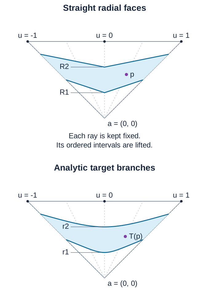
An exact two-dimensional instance. The centre is , the outer base is , , and the target radial heights are , . Subdivide the base at . The corresponding straight-face heights are , . The displayed lifting map is affine along each ray between the two straight faces. Curves are shown through their stated exact parametrizations; the picture is a sampled illustration, not a substitute for the proof.
For the original manifold input, this proves the global Euclidean relative construction and its restriction to a closed subanalytic subset. The complete globalization to an arbitrary real analytic manifold is proved below through finite-colour chart blocks, differentiable subanalytic cutoffs and analytic coordinate recovery on open simplices. The lower subanalytic prerequisites stated at the start of the relative construction remain explicit.
The signed normal-cone prerequisite
For a closed analytic submanifold , the normal deformation has central fibre , a parameter , and a map . In adapted coordinates , with , its maps are
Put . For any subset , its normal cone is
The closure is taken in the deformation manifold. For locally closed , make this definition in an open ambient neighborhood where is closed. The normal-geometry locality comparison makes it independent of that choice.
For two subsets, the diagonal construction gives
Thus the first member of the pair contributes with a plus sign. In a coordinate chart, the exact sequence criterion is
For , take . The scale tending to infinity is also valid at the zero vector; it is part of the prerequisite criterion. Exchanging the two sets in (5) negates the cone. These are positive-conic sets, with no assumption that they are vector subspaces or convex.
Normal-cone subanalyticity. If is subanalytic and is an analytic submanifold, then is subanalytic. If are subanalytic, then is subanalytic.
Proof. The maps in (3) are analytic. The lifted set is therefore subanalytic. Its closure and intersection with the analytic central fibre remain subanalytic by the set-operation input. For pairs, apply this argument to the diagonal and ; the latter is subanalytic by analytic inverse images and intersection. All assertions are local, so the same proof covers a locally closed . No image of a nonproper projection was used.
A curve that represents the exact limiting vector
Curve realization. Let be subanalytic and . There are analytic curve germs , both equal to at zero, lying respectively in for nonzero , such that
The coefficient of in (7) is exactly one.
Proof. In , consider
This is subanalytic by analytic inverse images and intersection. Criterion (6), with and , says that . Curve selection gives analytic through that point and in for . Set . Both required set memberships hold, and .
The analytic function is positive on both sides of zero and vanishes at zero. Hence
Choose the positive analytic -th root of near zero and put . Its derivative at zero is positive, so it has an analytic local inverse . After this reparametrization, and . The difference is therefore , which is (7) after renaming the parameter. This also works for . The even exponent is a consequence of this particular two-sided construction; the theorem only needs a positive integer.
If curves on are desired, choose a small interval on which the germs are defined and compose them with . This map takes into that interval and has Taylor expansion , so the coefficient and order in (7) are preserved.
The rescaling in (9) matters. Without it, a selected curve initially gives , with , and only a positive multiple of the specified leading vector has been normalized.
One-forms on a singular set
For an analytic one-form on , define to mean that its pullback to the analytic manifold is zero. This restriction is on tangent vectors, rather than the assertion that the ambient covector itself is zero.
Cone test. For a subanalytic set ,
This includes points in .
Proof. First we verify a density statement with its scales intact:
One inclusion follows from . For the other, use a sequence and scales representing a cone vector. Density of in lets us choose with , in a fixed local chart for large . Then and . This proves (11).
Suppose and belongs to . Apply (7) to and , using (11). We obtain
At nonzero parameter the curve is tangent to . Consequently . Analytic Taylor expansion gives
Divide by and let . The integer is nonzero, so . The zero vector is automatic, and empty cone fibres make no demands.
Conversely, at a regular point , every tangent vector to belongs to : realize it by a smooth local curve and apply (6). Thus the right side of (10) kills every such tangent vector, which is the left side.
For example, on the parabola , the nonzero ambient form vanishes on . At the origin its value is , which kills the horizontal tangent cone. Vanishing on a set is consequently weaker than vanishing as a section of the ambient cotangent bundle.
Analytic maps and locally finite unions
Pullback and union rules. Let be analytic and let , be subanalytic with . Then
If is locally finite and subanalytic, then vanishing on every implies vanishing on .
Proof. For , take a sequence and scales representing it. Taylor expansion at gives
Indeed, is bounded, so multiplying the first-order remainder by makes it tend to zero. Therefore . The cone test yields , proving (14).
Near a fixed point, a locally finite union has only finitely many members. Its point-normal cone is the union of their point-normal cones, because closure commutes with a finite union in (4). Apply (10) to each member and then to the subanalytic union.
In particular, vanishing passes to every subanalytic subset of , even a subset contained in its singular locus. This follows by taking to be the identity and .
Vanishing also passes to the closure. Here is the approximation argument, since uniformization applies to a closed set. For every ambient point ,
The inclusion from left to right is immediate. For the reverse, represent a vector by , scales , and . Choose with . Then and . Both sets are subanalytic, so the cone test proves if and only if . This uses approximation at the chosen scales; density alone without that estimate would not identify the cones.
The reverse direction needs surjectivity onto the set, but does not need an everywhere surjective differential.
Surjective detection. Under the same assumptions, if , then
Proof. Only detection remains. Set . The closure argument just proved gives . Choose a proper analytic uniformization with image . The manifold , like our other manifolds, is Hausdorff and countable at infinity. By (14), on .
Fix a regular point of and a neighborhood in which is a closed analytic manifold , of dimension . Shrink within that neighborhood if necessary. Then : taking closure introduces no new point inside a neighborhood where the set is already closed. Continuity gives , whereas implies that contains . Consequently the following map is analytic and surjective:
The open source manifold has a countable atlas. The classical Sard theorem therefore makes its critical values a measure-zero subset in each chart of . Surjectivity implies that a dense set of points has a lift with onto . At such a point, every has a tangent lift , and
Continuity makes zero everywhere. When the conclusion already holds, since tangent spaces are zero. This works near every regular point of , proving (16). The differential-topology inputs are Sard and the usual submersion criterion. Properness is used for the available uniformization, not imposed on ; we never assert that a nonproper analytic image is subanalytic.
Generalized conormals retain limiting normal covectors
For a locally closed subanalytic , define
The ordinary conormal on the right kills the tangent space of the regular locus. Its closure retains limiting covectors, while the last intersection restricts their base points back to . Formula (19) need not give the annihilator of at a singular point.
Generalized-conormal subanalyticity. The set is subanalytic.
Proof. Work in an ambient open set where is closed, and choose a proper uniformization with image . Let
Here is subanalytic. For each possible dimension of the regular locus, intersect its inverse image with . The regular dimension parts are subanalytic, and the rank conditions are semianalytic minors. Near a point mapping to the regular locus, the image of is tangent to that locus, so rank is exactly the surjectivity in (20).
The set is open in , because is open in and surjectivity is open over a fixed-dimensional manifold. Properness of implies properness on , so is subanalytic. The submersion theorem makes open in . It is dense there: over any regular neighborhood, is a surjective analytic map onto that neighborhood, and Sard shows that regular values are dense. Thus is also dense in .
Use the typed cotangent correspondence
The first map is a base change of the proper map ; hence it is proper on all of . Let denote the nonzero covectors over , as a subanalytic subset of , and set
Analytic inverse image, proper image and difference prove that is subanalytic. Explicitly, means that for every . Over at least one such lift exists and every such differential is onto . Consequently
The two conormal bundles over and have the same closure. To see the nontrivial inclusion, choose local conormal-bundle coordinates around a regular point, approximate its base point by points of the dense open , and keep the normal-fibre coordinates fixed. Every regular conormal covector is then a limit from . Taking closure in (23) and intersecting with proves (19) subanalytic. The normal-cone arguments earlier supplied a different construction; no equality between these two kinds of cone was assumed.
At the crossing , the generalized-conormal fibre at the origin is the union of the two covector axes. The point-normal cone is the union of the two tangent axes; the covectors annihilating all of it consist only of zero. These two answers encode different questions. A subsequent stratification includes the origin as its own stratum, whose ordinary conormal is the entire cotangent fibre.
Exercises with solutions
Two notions of a normal covector
Difficulty: Intermediate.
Compute and the annihilator of for . Then compute for . Compare its fibre at zero with the conormal of the point stratum.
Solution. Away from zero, the horizontal axis has conormal , and the vertical axis has conormal , where a covector is . Their closures give at zero. Every scaled displacement in lies on a tangent axis, and every vector on either axis is attained. Thus is their union. A covector killing both axes has .
For , the regular locus is , whose conormal is the zero covector. Its closure, restricted to , is the zero section over . In particular, (19) gives only zero at the endpoint. The conormal of is the whole one-dimensional fibre. The stratified conormal union therefore contains more endpoint covectors than the generalized conormal of the entire half-line.
A two-sided curve in a one-sided cone
Difficulty: Introductory.
Let . Compute . For every , give an analytic curve in for both signs of its nonzero parameter with leading coefficient . Explain why a nonzero first-order term cannot work.
Solution. Positive scales of positive points are positive, so every limiting vector is nonnegative. Conversely , realize , while , realize zero. Hence . The curve has exactly the required coefficient and belongs to for every nonzero . A real analytic function with nonzero linear term changes sign across zero. It therefore cannot remain in on both sides.
Quadratic tangency enlarges a pair cone
Difficulty: Advanced.
At the origin, compute for and . Compare it with the difference of their tangent spaces. Realize every vector in the answer by two analytic curves as in (7).
Solution. A difference from to has nonnegative vertical coordinate, and positive scaling preserves it. Therefore the cone is contained in . Given with , use
They lie in the respective sets and their difference is . For , take and . Evaluating at with scale proves the reverse inclusion, including the zero vector. Both tangent spaces at the origin are horizontal, so their difference is only the horizontal line. The pair cone also sees the second-order separation. Reversing the ordered pair gives .
An analytic image that escapes the properness hypothesis
Difficulty: Intermediate.
Show that the image of , , is not subanalytic in . Identify a compact set whose inverse image proves that is not proper.
Solution. If the image were subanalytic, its intersection with the analytic line would be subanalytic. That intersection is
Each member is an isolated connected component. Infinitely many approach the ambient point , so these components are not locally finite there. This contradicts the connected-component theorem, even though the accumulation point is not in the image. The compact rectangle has inverse image , which is noncompact. Thus the proper-image theorem does not apply.
Detection through a critical point
Difficulty: Introductory.
Let and , with analytic on . Prove directly that implies , although . Give a failure of detection when surjectivity onto the specified set is dropped.
Solution. The pullback is . Its vanishing gives for . Every nonzero is a nonzero cube, and continuity gives as well. Therefore . For failure, take a constant map , , and specify . Then whereas . Its image is , rather than .
A connected subanalytic set cannot vary under a vanishing differential
Difficulty: Advanced.
Let be connected and subanalytic, and let be analytic with . Prove that is constant on , without a properness assumption on .
Solution. The empty case is vacuous. The closure consequence of the cone test gives . Uniformize that closed set by a proper analytic . Rule (14) gives on , so is constant on each connected component. A second-countable manifold has at most countably many components: each is open and contains a member of a fixed countable basis, and different components contain different such members. Thus , and hence , is countable. It is connected because is continuous and is connected. A connected subset of containing two different points contains the interval between them, which is uncountable. Hence contains one point. This proof uses neither subanalyticity of nor properness of , and needs no triangulation.
Division at a normal-crossing boundary
Difficulty: Advanced.
Near , let be analytic functions and put , . Suppose as an analytic one-form. Show that for an analytic , and that and the tangential restriction of vanish on the normal-crossing set .
Solution. Comparing coefficients and cancelling analytic factors in the local ring gives
Thus both and divide . Expand as a convergent power series: divisibility by removes all terms of -degree zero and divisibility by removes all terms of -degree zero. Factoring leaves a convergent analytic series . Equations (26) give , . Hence on both axes. Along the tangent differential is , whose coefficient is zero; along it is , whose coefficient is zero. These are exactly the restrictions on the regular locus of the crossing. The cone test supplies the same vanishing at its singular point. This is the local division mechanism used when a resolved analytic function has monomial zeros.
Absorbing a unit while preserving two boundary axes
Difficulty: Intermediate.
For near , give analytic coordinates expressing as a sign times a monomial. Verify invertibility and preservation of both zero-set axes. Explain why the same coordinate step cannot make the nonconstant function into the monomial with every exponent zero.
Solution. Put , . Then . The Jacobian determinant is , which is positive; the inverse is , . Thus both axes and their crossing remain the same sets. An all-zero-exponent monomial is constant. If became constant after a coordinate change with an inverse, composing back would make constant on an open neighborhood, contradicting its nonzero -derivative. The point of the unit lemma is the available positive exponent at a zero, not an assertion that every unit is constant in suitable coordinates.
Centres, parallel directions and a projection-open enlargement
Difficulty: Intermediate.
Let be the union of the two axis segments in . Determine its singular lines, choose a centre from which every line has finite intersection with , and choose a good parallel direction. Then explain why the projection of the one-point set to the first coordinate is not open and give a compact finite-fibre enlargement whose projection is open near that point.
Solution. An interval in lies on one of its axes, so the only singular lines are the two coordinate axes. Any centre with both coordinates nonzero, for example , lies on neither; a line through it cannot coincide with an axis and meets the two segments in at most two points. The direction is nonsingular for every translate: its lines are parallel to neither axis. In contrast, either axis direction has a singular translate. The image of the one-point set is , which is not open in the base line, although the singleton is open in its own subspace topology. The enlargement has one-point vertical fibres and open projection near the origin. Projection openness is local here; at its two endpoints the map to the whole base line is not open. The example also shows that an enlargement may have larger dimension than the original set.
Reciprocal heights and the exact radial lift
Difficulty: Advanced.
Use the two target branches in the figure, with base subdivided at . Compute the straight heights on . On the ray , compute the domain and image of the midpoint between the two straight faces under the lifting map. Explain why averaging the vertex heights would not describe a straight face.
Solution. On that base interval the vertex weights are . The lower vertex heights are , and the upper ones are . Therefore
At , these are , and their midpoint is . Thus the domain point is . The target heights are . Since the map is affine on this radial interval, its midpoint has height , giving . Both points lie on the ray with base . The arithmetic average of the lower vertex heights is , whereas the straight face has radial height . The difference comes from radial projection: the affine coefficients of a point in the straight face are proportional to , rather than to the base weights themselves. This is the reciprocal-height calculation in the proof.
Resolving a function whose real zero set already crosses normally
Difficulty: Advanced.
For , compute . Let
Prove that is an analytic manifold, that is proper and is an analytic isomorphism over , and that has the required sign-monomial coordinates near every point of .
Solution. The derivatives are
The real zero set consists of the axes. On , the second derivative is ; on , the first is . Thus the zero-critical set is exactly .
On the projective chart , put and . The incidence relation says , so are unrestricted analytic coordinates. On , put and ; there , with analytic coordinates . On their overlap the transition is
with nonzero determinant . These charts cover , including its whole exceptional fibre over the origin. They make it an analytic two-manifold and make analytic.
The incidence set is closed in : in each projective chart it is the zero set of the displayed continuous equation, so its complement is open. The projective line is compact, being the quotient of the unit circle by its antipodal involution. For compact , the set is consequently closed in the compact product and is compact. Hence is proper. It is surjective; the origin has a projective line of preimages, and each nonzero has the unique preimage with direction . The inverse is analytic on the punctured plane, as one sees on and . This proves the isomorphism over precisely the required complement.
In the first chart,
At the exceptional point , set , . The Jacobian determinant there is one, the axes are preserved, and . At with , let and shrink so that keeps this sign. Use coordinates
The root is positive and analytic, the Jacobian determinant at the point is , and .
The second chart supplies the remaining direction :
At , set , , giving with invertible Jacobian. If , set , ; the expression becomes . Thus every point of has a sign-only coordinate monomial. Only the two axis directions require two positive exponents; every other exceptional direction requires one. The real zero-set picture had concealed the extra vanishing factor, and the complete two-chart construction retains it.
Coefficients, a cusp and an unresolved exceptional tangency
Level: advanced. For marked with , compute its coefficient conditions, the two charts of the blowing-up of the origin, and the order at the exceptional points. Explain why the first multiplicity drop does not yet give normal crossings of the total function divisor.
Solution. The distinguished derivative is ; , with mark , and with mark . The coefficient order is at least two only at , so the equimultiple locus is the origin. The coefficient’s normalized order there is .
In the chart, . The total and controlled transforms are
The transformed coefficient is with mark , exactly , so its order has dropped below its mark. At the exceptional point , has order one because . At an exceptional point with , is a unit. In the chart, , the controlled transform is ; it is a unit on the entire exceptional line . These computations cover every projective direction.
The strict transform is smooth but tangent to the exceptional line at the origin. Their differentials there are proportional. Thus their union is not normal crossing, despite the distinguished multiplicity having dropped from two to one. The total transform retains the exceptional exponent two. Both the exceptional-incidence conditions and the coefficient weights must remain visible in the resolution algorithm.
The necessary gradient exponent on a flat direction
Level: intermediate. For , prove a local Łojasiewicz gradient inequality with exponent , and show that a smaller exponent cannot hold in any neighborhood of the origin.
Solution. The Euclidean gradient is . For , concavity of the power gives
For completeness, subadditivity , , follows by fixing and differentiating for : its derivative is nonpositive, so its value is at most . The last inequality uses and .
On , an inequality would require . If , its left side tends to infinity as , which is impossible. Thus the flat direction determines the necessary exponent. The full gradient theorem in the human component explains why some rational exponent below one exists; this calculation determines the optimal exponent for this function.
Formal replacement and signed analytic normalization
Exercise 14 (intermediate). Explain why the formal linear convergence theorem does not claim convergence of every formal solution. Give a divergent formal solution of in , and a convergent solution with the same jet through any fixed degree. For , , normalize by the coefficient of largest absolute value, using the coefficient at a tie. Determine the normalizing parameters and a uniform bound on the order in .
Solution. Let
The difference is coefficientwise. For any , the absolute terms of have ratio , which eventually exceeds two. They therefore do not tend to zero, so this series has convergence radius zero. Both components of the displayed formal solution diverge.
For any fixed , put . The pair is a polynomial solution and agrees with the formal pair in degrees . Thus a convergent replacement can preserve every prescribed finite jet, although there is no single convergent series with all those Taylor coefficients. The distinction persists even for this elementary finite linear equation.
For the second part, , , and the units are . On , take , . Then
The first parameter takes both signs. Restricting it to would omit positive . On the correct signed compact interval, everywhere. Therefore the order is at most one uniformly; at it is exactly one, and elsewhere it is zero. This verifies the derivative criterion even where the normalized value itself vanishes.
References and the next cotangent question
Bierstone–Milman, Semianalytic and subanalytic sets, Definition 3.1 and §§3, 5 and 7, treats the local projection language, complement theorem, proper uniformization and fixed-dimensional regularity. Proposition 3.12, printed pp. 19–20, gives a dimension-preserving analytic presentation. Theorem 5.1, pp. 30–32, proves analytic-set uniformization using normal-crossing charts and induction through lower-dimensional centres; the deduction for closed subanalytic sets follows on p. 32. The torus argument here uses a compact fibre extremum and squared differential minors to reduce the source dimension directly from the proved function resolution. The uniformization conclusion supplies a proper map onto the set; the separate function-resolution theorem also retains its asserted isomorphism away from the singular zero set.
Valette’s On subanalytic geometry, §1.2 and §§2.1–2.2, supplies finite analytic cells, definable derivative tests and the choice-plus-Puiseux route to analytic curves in the globally subanalytic setting. The bounded-chart comparison is what permits their use on the local sets here. The two-sided curve and exact leading-vector normalizations are then checked in this lesson. The linked adapted components retain Valette’s attribution and CC BY 4.0 terms.
Shiota’s relative polyhedron proof is the triangulation source described above. The later manifold argument proves its globalization through finite-colour chart blocks, finite-regularity subanalytic cutoffs and analytic coordinate recovery on open simplices; its specific Kankaanrinta and Milnor credits appear at those constructions. The arbitrary-manifold conclusion is therefore proved here from the stated lower inputs. The separate function-resolution proof proceeds through the marked coefficient construction, recursive exceptional histories, analytic thresholds, closed canonical centres, compact-fibre termination, and proper gluing of the independently matched local towers.
For the cotangent setting, Kashiwara–Schapira’s freely readable Microlocal Study of Sheaves, §§8.1–8.2 explains how Whitney limits control conormals and how isotropic sets lie in conormal unions. Its §8.2 convention restricts “subanalytic set” to locally closed sets, so it is not a substitute for the arbitrary-subset calculus used here. Our closure and surjective-detection proofs retain that broader stated scope and use the explicit curve and uniformization inputs; they do not require triangulation.
Guillaume Valette’s On subanalytic geometry, §2.2, supplies the separately licensed choice, curve-selection and Łojasiewicz treatment linked above. The linked analytic preparation treatment now proves its Chapter1 cell, complement and Puiseux inputs in the projective product convention. The local comparison here proves the manifold curve-selection consequence without a global definability assumption. The marked coefficient argument proves the local dimension reduction and its test-transform persistence. Higher analytic prefixes, current history, and rebirth supplies the recursive exceptional histories, and Finite termination over a compact fibre proves termination for the local towers used in the proper global construction.
For the next step, take the canonical one-form on . Its vanishing on a positive-conic subanalytic set defines isotropy. The cone test and surjective detection just proved will then turn cotangent correspondences into rigorous statements about isotropic images and stratifications.
Further exercises on preparation
15. A bounded function that needs a negative preparation exponent
Level: advanced. On
consider . It is positive and bounded. Show that a finite preparation of cannot have only nonnegative last-coordinate exponents, even if translations and analytic units are allowed. Use the convergent Puiseux theorem proved in the analytic preparation treatment.
Solution. We have . The formula is already a reduction with translation zero, unit one and exponent .
Suppose there is a finite cell preparation with all exponents nonnegative. Refine its one-dimensional base and shrink so its base interval next to zero is . Over it, list the finitely many endpoints within the original band, including and :
Duplicate endpoints are removed; every open interval between consecutive endpoints is a preparation cell. Each positive endpoint has a convergent Puiseux expansion with leading term , where . The bounds force . Since and , some consecutive pair has strictly decreasing leading order. Thus .
On the corresponding band, write the supposed reduction as
The coefficient cannot vanish, since . The center is outside the band, hence either or throughout this connected base interval. After shrinking it, take
The actual ratio is
If , the distance ratio is at least one, so the prepared ratio is at least . If , then
so the prepared ratio is at least . Both contradict its limit zero. Some negative exponent is therefore necessary. Boundedness of the whole function does not force nondegenerate preparation; its base coefficient can compensate for an inverse power on a narrowing band.
16. Even substitutions and parameter-dependent poles
Level: intermediate. Explain why the substitution does not make analytic on a two-sided neighborhood of zero, while does. Then analyze the globally subanalytic function
Give one common root-variable Laurent expansion and one even substitution that agrees with the actual function for both signs of the new variable. Determine the parameter pieces on which a continuous analytic extension at zero is possible.
Solution. The two compositions are and . A two-sided analytic substitution must make every cleared exponent even, not merely make the substitution exponent even.
With on the positive -axis the Laurent expansion is
For both signs, choose . Then
For the pole remains; no continuous extension is possible there. On the parameter cell , the function becomes , analytic across zero. The cells give one finite analytic parameter partition.
Even at , continuity fails if one keeps all parameters together. Along , the first summand equals and diverges. The continuous-parameter theorem requires joint continuity on its stated neighborhood; continuity on the one slice does not supply that hypothesis.
Compatible triangulations on arbitrary analytic manifolds
Manifold triangulation theorem. Let M be a Hausdorff second-countable real analytic manifold without boundary, of finite dimension, and let its subanalytic subsets form a locally finite family. There is a countable locally finite linear simplicial complex with closed support in a finite Euclidean space and a subanalytic homeomorphism from that support to M, compatible with the family. On every open simplex the map is an analytic diffeomorphism onto an analytic embedded submanifold.
We prove the globalization from the relative polyhedron theorem above. The proof includes the finite-colour covering lemma, finite-regularity subanalytic cutoffs, a proper embedding, bounded proper-image calculus, the extraction of a closed subcomplex and analytic chart-coordinate recovery. The relative theorem’s expressly stated lower prerequisites remain in force. They are separate from the elementary covering and cutoff arguments proved here.
Finite-regularity subanalytic cutoffs on arbitrary analytic manifolds
This is a bounded teaching proof for the cutoff and partition-of-unity dependency in the SH-03 manifold embedding construction. It treats Hausdorff, second-countable, finite-dimensional real analytic manifolds. Fix a finite integer . Every function constructed below is , and its graph is locally semianalytic, hence locally subanalytic, in the indicated analytic manifold. The word “subanalytic” here concerns every ambient point of that graph; it does not assert a single globally definable Euclidean presentation at infinity.
Related cutoff constructions are treated in Marja Kankaanrinta, A subanalytic triangulation theorem for real analytic orbifolds, arXiv:1105.0209v2, §5. Its closed-set separation lemma cites Proposition 5.4 of Kankaanrinta’s 1991 dissertation. The proof below supplies the manifold separation and support construction directly, without taking that unread proposition as a prerequisite. It also supplies the finite regularity needed for the embedding’s differential-rank argument. Kankaanrinta’s §5 is the comparison source for the construction, not the source of this stronger stated regularity.
Statements and support convention
For a function on , write
The following statements will be proved.
- Every open cover of , with no subanalyticity hypothesis on its members, admits a countable , locally subanalytic partition of unity . Each support is compact, lies in one analytic chart and in one member of , and the support family is locally finite in .
- For arbitrary disjoint closed subsets , there is a , locally subanalytic with and .
- If is closed and , where is open, there is a , locally subanalytic with and . If is compact, can have compact support in ; if lies in an analytic chart, that compact support lies in that chart.
Compactness in statement 3 requires a compact inner set. If is noncompact, a compactly supported function equal to one on is impossible. The general statement instead supplies a support contained in a locally finite union of compact coordinate-ball supports. All partition members in statement 1 individually have compact supports.
The empty manifold and an empty inner set have the empty partition and zero cutoff, respectively. All remaining arguments assume the relevant set is nonempty.
1. The compact radial bump, including derivative checks
Choose rational data and in . Set , , , and . For a real variable , define
The denominator is strictly positive for every real : if , then ; if , then ; and between and both are positive. Thus
The graph of this function is semialgebraic: on the three polynomial-inequality regions it is specified by , with , and , respectively. Overlapping endpoints give the same value. Non-strict inequalities are expressible using strict inequalities and equalities. Consequently, no projection theorem or o-minimal result is needed for this graph description.
The function is . Indeed, its derivatives through order on the positive half-line are constant multiples of , which tend to zero at the origin, matching the zero derivatives on the negative half-line. Its quotient in (C1) is therefore . Equivalently, near from above,
and near from below,
Since , these expressions have zero derivatives of all orders at their joining endpoints. In particular, for the required case , and more generally for ,
and outside this interval and at both endpoints. The displayed derivative tends to zero there.
Let be an analytic chart such that . Define
On , composition with the analytic squared norm makes a function, equal to one on the closed inner ball and strictly positive exactly on the open outer ball. In chart coordinates its gradient is
which tends to zero at both joining spheres. Its support in is exactly
This is compact and therefore closed in the Hausdorff manifold , and it lies in . Every point of , including every point outside , has an open neighborhood disjoint from ; on that neighborhood . Thus zero extension introduces neither a continuity nor a differentiability defect at the chart boundary.
The graph is locally semianalytic on , by the three analytic branch conditions from (C2) with ; at every point outside , the graph is locally the analytic zero graph. These cases cover all ambient graph points, so is locally semianalytic and locally subanalytic globally on . A different analytic chart does not change this conclusion: analytic coordinate transitions substitute analytic functions in the finitely many local equations and inequalities. The construction also works for a zero-dimensional chart, where the coordinate ball is the singleton .
2. A countable locally finite nested coordinate-ball refinement
We prove the topological refinement needed above instead of assuming an analytic partition of unity or requiring a cover member to be subanalytic.
First, there is a countable cover by open coordinate balls with compact closures in . For every point, take a coordinate ball whose closed coordinate ball lies in a chart image; its closure in is compact. Second countability gives a countable subcover: for each basis element contained in some member of this cover, select one such member. The selected members cover because a point and a covering neighborhood contain an appropriate basis element. This argument also proves the particular Lindelöf assertion being used.
Construct compact sets , , with
where . At stage , cover the compact set by finitely many precompact open coordinate balls, and let be the union of their compact closures. The original open balls are an open subset of this union containing the target compact set, which proves its inclusion in . The resulting need not be subanalytic. They are only used to organize the choices.
Given any open cover , put
The sets are compact and cover : for any , its first membership in some places it in . Also , since and .
At , choose containing and an analytic chart around . The intersection of this chart, , and is open. In its chart coordinates, choose a rational center and rational such that the inner ball contains the coordinate of and the closed outer ball lies in that intersection. To justify the rational choice, first take a small Euclidean neighborhood contained in the target open set, then take close enough to the coordinate of , and choose rational radii satisfying
with smaller than the remaining distance to the boundary of the chosen Euclidean neighborhood. Density of the rationals provides such data.
By compactness, finitely many resulting inner balls cover . Write them as and their corresponding compact outer balls as , . We have
and every lies compactly inside an analytic chart. The family of all is locally finite in . Indeed, if , this open neighborhood is disjoint from for every , because those balls avoid . Only finitely many earlier levels remain, with finitely many balls at each level. The inner balls cover , and the family is countable.
This proves precisely the needed refinement by nested balls with locally finite compact outer closures. It uses only second countability, the Hausdorff condition, elementary coordinate topology, and finite subcovers of compact sets.
3. Local graph calculus, with the boundedness hypotheses made explicit
For the particular radial bumps and their combinations, even the full general subanalytic image calculus can be avoided. Near any point, only finitely many compact supports from (C8) meet a neighborhood. A member whose support misses the point is identically zero after a further shrinking. For every other member the point lies in its analytic chart. Intersecting these finitely many neighborhoods gives a neighborhood on which each bump has finitely many semianalytic branches with an analytic expression. On a middle branch that expression is rational in analytic functions and its denominator is positive on the branch, as in (C2). Refine by the finitely many simultaneous branch choices. Each resulting piece is semianalytic, and sums, products, and quotients with a positive denominator have analytic expressions on a neighborhood of that piece. Their graphs are specified by analytic equations, or by the same equations after clearing positive denominators. Finite union gives a locally semianalytic graph. This observation will cover all the cutoffs, separation functions, and partitions constructed below.
Here are the corresponding general local subanalytic graph statements useful for other parts of the embedding argument. In these statements functions are continuous; this ensures bounded auxiliary graph coordinates near a fixed point.
G1 — finite tuples. If continuous have locally subanalytic graphs, then the graph of is locally subanalytic. In local coordinates, it is the intersection of the analytic inverse images of under . This uses finite intersection and analytic inverse-image closure.
G2 — sums and products. If are continuous with locally subanalytic graphs, then and have locally subanalytic graphs. Fix , take a relatively compact coordinate neighborhood , and shrink it so are bounded on a neighborhood of . Take bounded open auxiliary intervals containing their ranges there. Intersect the two graph conditions and the analytic equation , respectively , inside these bounded coordinates, also bounding . This subanalytic set has compact closure in a larger chart-and-interval neighborhood. Projection to is analytic and proper on that compact closure, so its image is subanalytic near . The projection describes exactly the desired graph. The properness on the closure, not just on the graph set, is the relevant image hypothesis.
G3 — reciprocal and division. If is continuous, locally subanalytic, and nonzero everywhere, the graph of is the analytic inverse image of under , on the open manifold . At an ambient point with , continuity of makes bounded near its base point, so reciprocals cannot approach zero there; the graph is locally empty. Alternatively, near , is bounded above and bounded away from zero, and the bounded graph projection argument applies. Together with G2 this proves the division statement. A positive continuous denominator admits these local bounds even if its global infimum is zero.
G4 — analytic compositions. A continuous locally subanalytic map composed with an analytic map defined on a neighborhood of its local image remains locally subanalytic. Use G1 and the graph equation , restricting to a compact neighborhood of the image and to bounded coordinates, and project as in G2. Analytic chart changes and products with analytic chart coordinates are special cases. For the constructed piecewise analytic functions these cases also follow directly from their finite branch equations.
G5 — locally finite sums. If is a family of locally subanalytic functions with locally finite supports in the ambient manifold, then is and locally subanalytic. Around every point, all but finitely many functions vanish on one neighborhood, so this is a finite sum there. The assertion concerns supports, not merely a pointwise finite count of nonzero values. Derivatives through order are those of the finite local sum.
G6 — controlled zero extension. Let be open and let be and locally subanalytic. If
then extending by zero to preserves both properties. On there is no change; each point outside lies in the open set , where the extension is identically zero. Compact containment is a sufficient instance of (C9), not a replacement for local subanalyticity of the original graph. In particular, if has compact support in an analytic chart , the zero extension of is and locally subanalytic by G2/G4/G6. Chart coordinates may be unbounded towards the chart boundary, but every point of that boundary has a neighborhood where this product is zero.
The general facts G1–G4 use the exact lower-calculus prerequisites
“finite intersection,” “analytic inverse images,” and “analytic images
proper on the closure,” used here with their precise conditions: finite
intersections and analytic inverse images preserve local subanalyticity;
an analytic image is locally subanalytic when its restriction to the
closure of the source set is proper. G5 and G6 are proved here from
locality. Their globally subanalytic Euclidean analogues are actually
read in Guillaume Valette, On subanalytic geometry,
arXiv:2507.23622v1, native analytic_geometry.tex, lines
61–127 (graph definition and Basic Properties). Those global analogues
are not applied to an arbitrary open cover or to the whole manifold. The
direct finite-branch argument at the start of this section makes the
present partition and cutoff conclusions independent of these deeper
general closure theorems; they need only the elementary inclusion of
semianalytic sets among subanalytic sets.
4. Partition of unity subordinate to an arbitrary open cover
Apply Section 2 to , and index the chosen pairs of nested balls by . Let be the bump from Section 1, equal to one on the corresponding inner ball and supported on its compact outer ball . Define
The sums are locally finite in a neighborhood, so is and locally semianalytic by Section 3. Some inner ball contains every , and its bump equals one there, hence . Division preserves regularity, and the finite branch descriptions prove each quotient locally semianalytic. Alternatively, G3 proves local subanalyticity directly. Thus
The support equality holds because is strictly positive: exactly where . These supports are compact, contained in analytic charts, and locally finite. They cover since at every point some is positive. This proves statement 1, including all support and smoothness conditions.
If a partition indexed by the original cover members is wanted, choose the recorded assignment and put
It is and locally subanalytic; only countably many members are nonzero. Its support is contained in and the grouped support family is locally finite. To check this last support assertion rather than assume it, a locally finite union of closed sets is closed: near a point outside the union, first discard all but finitely many sets using local finiteness and then avoid those finitely many closed sets. Therefore the union of with is a closed subset of containing . A neighborhood meeting only finitely many can meet only the finitely many grouped supports with their labels. Grouping can lose compact support in one chart, so the refined partition (C10) is the version used when those conditions matter.
5. Arbitrary closed-set separation without realizing an arbitrary zero set
For disjoint closed , the two open sets
cover . Apply the refined partition of Section 4, with each support assigned to one of these two sets. Write for indices assigned to , and put
This is a locally finite sum, is and locally subanalytic, and lies in . At a point of , every term in this sum vanishes, since its support is disjoint from ; hence . At a point of , every partition term assigned to vanishes, so the remaining terms sum to one; hence . This proves statement 2.
In particular, we never cover all of by a support family that is locally finite in and demand positivity at every point there. Such a construction would force , an unjustified condition for an arbitrary closed set. In (C12) the zero set merely contains and the one set contains . The arbitrary sets are inputs to open-neighborhood choices, not analytic graph constraints.
6. Cutoff plateaus and the nested-shrink use
Let with closed and open. Apply Section 4 to the open cover . If consists of indices assigned to , set
Exactly as in Section 5, , is and locally subanalytic, and . The closed, locally finite union lies in , so
This proves the general cutoff assertion. Notice that zero values on , by themselves, would not establish (C14); the locally finite closed union is the support control.
There is a shorter compact construction that also gives a plateau on an open neighborhood of . If is compact, choose finitely many nested coordinate balls with outer compact balls contained in and with inner open balls covering . Let their bumps be , and set
Each factor lies in , so . On every inner ball some , hence . Outside the finite union of outer compact balls all , hence . The finite union is a compact subset of . Finite products preserve regularity and the local finite branch graph description. Thus (C15) is a compactly supported , locally subanalytic cutoff equal to one on an open neighborhood of . When lies in one analytic chart, all the balls can be selected in that chart, so the support lies compactly inside it. One can also form the product locally for a locally finite ball family, but the partition proof (C13) already supplies the general noncompact statement.
For the intended nested-shrink application, assume
Formula (C15), applied to , gives
with regularity and a locally semianalytic graph. Here means that is compact and contained in ; need not be subanalytic. If a locally finite family and compact inner sets are supplied, construct independently this way. The supports remain locally finite because they are contained in . If the inner sets cover , then , and (C10) with in place of gives the desired partition. This applies to a finite-color family just as to an uncolored locally finite family; no coloring hypothesis enters the cutoff proof.
Finally, for each chart , the vector map
is and locally subanalytic by the finite branch equations or G2/G4/G6. On the plateau neighborhood it equals , with exactly the chart’s derivatives. This is the cutoff fact needed for the later embedding and coordinate-recovery argument; the embedding itself is outside this bounded proof.
7. Optional finite-group chart statement
Suppose a finite group acts analytically on , and are invariant disjoint closed sets. Apply Section 5, then average:
This function is invariant, , locally subanalytic, still in , and has the same prescribed zero and one values. Analytic diffeomorphisms preserve the local finite branch equations; the finite sum preserves all regularity. Likewise, if are invariant and a compact cutoff is available, the average is one on and has support contained in the finite compact union . This supplies a bounded finite-group lift of the separation/cutoff fact. No full orbifold atlas-gluing or global quotient theorem is claimed here.
Exact dependency boundary
For the constructed partitions and cutoffs, the dependencies are finite-dimensional analytic chart topology; second countability and Hausdorff compactness; density of rational coordinate data; finite subcovers of compact sets; elementary differentiation and division by a nonvanishing function; the definition of locally semianalytic sets and its invariance under analytic coordinate changes; and semianalytic inclusion in the local subanalytic class. The compact-exhaustion and locally finite refinement steps are fully proved in Section 2. No analytic partition of unity, analytic embedding theorem, arbitrary globally definable cover, or prescribed subanalyticity of an arbitrary open/closed input set is assumed. General local graph consequences G1–G4 additionally use only the lower calculus stated with its proper-on-closure condition in this lesson; those deeper statements are not needed for the explicit finite-branch construction.
Finite-colour refinement for a manifold
This is a complete proof of the manifold case needed by SH-03. It applies to a topological manifold; no differentiable structure is required. The auxiliary nerve need not have a global dimension bound. The construction never triangulates the manifold.
Statement
Let be a second-countable Hausdorff topological -manifold, , and let be any open cover. Then there is a countable locally finite open refinement
which covers , such that distinct members of each are disjoint. We can require more: for every there are an original cover member and a prescribed-atlas chart domain such that
Thus the statement requested for a second-countable Hausdorff paracompact manifold follows. Paracompactness need not be used separately: the elementary exhaustion below provides the needed locally finite covers. The empty manifold is immediate. The usual convention here is that manifold charts are open subsets of , so no boundary is involved.
Source comparison and attribution
Marja Kankaanrinta, A subanalytic triangulation theorem for real analytic orbifolds, arXiv:1105.0209v2, Section 2, states the finite-colour theorem for a paracompact space of covering dimension , attributes the result originally to J. Milnor, and also credits R. S. Palais. Its next paragraph explains the indexing by finite unordered tuples.
John Milnor’s Differential Topology, Princeton lectures, Fall 1958, notes by James Munkres, Lemma 2.19, gives the colouring by strict inequalities between partition coordinates. That text assumes the covering-dimension bound for a manifold. The actual source was read at the opening page (attribution and chapter structure) and printed pages 18–19, especially Lemma 2.19 on printed page 19, PDF page index 18. Available lecture notes.
The strict-inequality colouring in the last section below is this Milnor construction, with its openness and local finiteness checked explicitly. The missing manifold dimension input is supplied here by a proved local approximation lemma and a locally finite elimination of nerve simplices. The resulting proof is an elementary argument. In particular, Palais’s theorem and an asserted equality of manifold and covering dimensions are not dependencies of this proof.
1. Locally finite compact chart supports
We first construct the elementary neighbourhood data used twice in the proof.
A point in an open set has nested chart cubes such that
Indeed, restrict a chart around the point to , and choose two nested Euclidean open cubes whose closures lie in its coordinate image. Their closed-cube inverse images are compact and hence closed in the Hausdorff space ; they are consequently the closures in . The chart may be chosen from a supplied atlas and restricted. The same argument works for , when a chart cube is a single isolated point.
There is a countable cover by such relatively compact chart neighbourhoods. To see the countability, a second-countable space is Lindelöf: from an open cover, select one cover member for each basis element which lies in a cover member. These selected members still cover. Apply this to the cover of all the neighbourhoods just constructed.
There are compact sets , , with
Inductively cover the compact set by finitely many relatively compact chart neighbourhoods and let be the union of their closures. The open neighbourhoods in that finite cover show that . The sets are compact, and every is eventually in an interior. Set for negative .
The compact band
lies in the open set
For every point of , use (F2) inside , with containing the point and a chosen atlas chart containing it. Select finitely many inner cubes covering , and retain their paired outer cubes . Enumerate the pairs as , where is finite or countable. They satisfy
The outer family is locally finite. If , the neighbourhood meets none of the cubes belonging to a band , because these cubes avoid . Only finitely many smaller bands exist, and each contributes finitely many cubes. In particular every compact set meets only finitely many : use finitely many of these local neighbourhoods to cover the compact set.
Within the coordinates of , take a continuous product of one-dimensional hat functions which equals one on and vanishes outside a smaller closed cube inside . Extend it by zero to . This gives
The zero extension is continuous, since its support is contained in the interior of its chart domain. The family of supports is locally finite. The sum is therefore continuous and positive, and
is a continuous partition with compact chart supports. All sums are finite on a neighbourhood of each point. This constructs the partition needed here, rather than invoking a partition-of-unity theorem.
Exactly the same construction applies to any open submanifold , using its own compact exhaustion. It supplies a locally finite family of closed inner cubes covering , continuous functions equal to one on those inner cubes, and larger compact chart cubes containing their supports.
2. A proved point-avoidance approximation lemma
Lemma. Suppose is a second-countable Hausdorff topological -manifold, , is continuous, , and is continuous. There is a continuous with
Local approximation. On a closed Euclidean -cube , every continuous map to can be approximated uniformly within any by a piecewise affine map missing . Subdivide into a sufficiently fine finite cubical grid. Each small grid cube is divided into the simplexes obtained by ordering its coordinate increments; these divisions agree on shared faces. Uniform continuity makes the oscillation of on each small simplex less than .
Choose the images of the finitely many vertices within of their original images, as follows. When a new vertex image is chosen, avoid the affine spans of together with each collection of at most previously chosen vertex images. There are finitely many spans, each of dimension at most . A proper affine subspace is closed with empty interior; a finite union of such subspaces cannot contain a nonempty open ball, by successively choosing a smaller open ball disjoint from each subspace. Thus a permissible new image always exists in the required small ball. The construction ensures that together with any at most chosen vertex images is affinely independent.
Extend the vertex images affinely over each simplex. The extensions agree on faces. No simplex image contains , because that would put in the affine span of at most of its vertex images. Barycentric interpolation and the oscillation bound give uniform error less than . This is only an explicit finite decomposition of a Euclidean cube, not a triangulation of .
Global construction. Use the end of Section 1 on to obtain closed inner chart cubes covering , larger closed chart cubes , and continuous functions such that
Choose these so that the family is locally finite. Put . Inductively choose satisfying
and, when ,
The second minimum is positive by the preceding stages and compactness. Empty unions impose no condition. Approximate , in its chart coordinates, by a piecewise affine map missing with error less than , and define
The formula is continuous across the boundary of , since vanishes on a neighbourhood of that boundary. On , the new map equals and avoids . Condition (F9) preserves avoidance on all earlier . Hence avoids on .
Every point has a neighbourhood meeting only finitely many . Thus is eventually constant on that neighbourhood, and the pointwise limit is continuous. Each point belongs to some , and its final value is a finite-stage value after stage ; it still avoids . At a point changed at stage , (F8) bounds the change by . Therefore
This proves the lemma. It uses neither Sard’s theorem, a smooth approximation theorem, the Baire theorem, nor covering dimension.
3. The nerve is locally finite, and the partition map is proper
Let be the nerve of the cover : a nonempty finite set of vertices is a simplex when . Its realization consists of the finitely supported vectors
in , with the subspace topology. This agrees with the usual simplex topology for this locally finite complex.
In fact each vertex belongs to only finitely many simplexes. The compact set meets only finitely many cover members; any simplex containing has all its vertices among these finitely many neighbours. There are only finitely many such finite vertex subsets. This proves local finiteness of the complex, but does not supply a uniform bound on its simplex dimensions.
Here are the topology details we will use. At , choose an index with . The open neighbourhood
meets only the finitely many simplexes containing . It lies in a finite subcomplex; its closure lies in a compact union of finitely many closed simplexes. Thus is locally compact and Hausdorff. The same finite-subcomplex description proves agreement of the two topologies. A compact subset of lies in a finite subcomplex: cover it by finitely many neighbourhoods (F11), then take the union of their finite subcomplexes.
The functions (F6) define a map
Its support is a simplex because implies . Continuity follows from the fact that locally only finitely many of the occur. If a compact set lies in a subcomplex with finite vertex set , then
The inverse image is closed and the right side is compact, so is proper. It is also a closed map: for a closed and , take a compact neighbourhood of . The set is compact and closed, so its complement in the interior of gives a neighbourhood of missing . In particular is closed in .
The same argument applies to any continuous for which
Such a map remains proper and closed. We will maintain this support condition during the compression. Properness is verified here because it is useful to the intended nerve route; point avoidance itself was proved in Section 2 and does not require closedness of the image.
4. Compress into the -skeleton without enlarging supports
We explain one simplex removal first. Let be a subcomplex, let be a maximal simplex of with dimension , and let be continuous. Choose , for example its barycentre, and put
The interior of this maximal simplex is open in . Indeed, near an interior point all its vertex coordinates are positive; any simplex with those coordinates positive must contain , and maximality forces it to equal . Therefore is an open -manifold. If is empty, the simplex may simply be removed.
Otherwise identify the affine span of with . Apply Section 2 on to , the point , and the continuous positive tolerance
We obtain . The image stays in the simplex interior because its displacement is less than the distance to the boundary. Define on and elsewhere. This extension is continuous: at , continuity and closedness of give ; as tends to , the bound (F15) tends to zero. The modification has not changed any coordinate outside the carrier , nor introduced or removed vertices within its interior. Thus
and it is unchanged elsewhere. The map now misses everywhere.
Radially retract to its boundary. In the vertex coordinates of , with , write
The maximum is positive for , because the coordinates of both and sum to one. Since , the ray reaches the simplex boundary at this parameter; every coordinate of is nonnegative, at least one is zero, and their sum is one. If , some , so and . The formula is continuous away from .
Extend by the identity outside . This is a continuous map on : the two closed pieces and agree on the boundary. Hence
is continuous, where removing the maximal simplex means removing its interior while retaining all its proper faces. It satisfies
At a point changed by (F17), its former carrier was exactly ; the radial retraction replaces this carrier by a proper face.
We now perform such removals for all simplexes of dimension greater than . Their dimensions may be unbounded. An ordinary instruction to start at a highest dimension would consequently be invalid. Instead enumerate these simplexes in an arbitrary fixed countable list, and repeatedly remove the first unremoved simplex in that list whose proper cofaces have all been removed.
This process is well defined and eventually removes every listed simplex. Each simplex has only finitely many cofaces, since any one of its vertices belongs to only finitely many simplexes of . Among the unremoved cofaces of any unremoved simplex, a maximal one is available for removal. To see eventual removal, induct on the maximum length of a proper-coface chain above a given simplex. Maximal simplexes are immediately available. Once the finitely many proper cofaces of a simplex have been removed, it is available permanently, and only finitely many entries earlier in the fixed list can precede it. Thus it is removed after finitely many more steps. This induction has finite height for each simplex, even though heights are not globally bounded.
Starting with , apply (F17) at these stages. Denote the successive maps by . Their supports decrease pointwise. At a given , choose a neighbourhood meeting only finitely many , with their indices in a finite set . Throughout the construction every image of a point of has its support in , by (F18). A simplex removal can change that map on only if all vertices of the removed simplex belong to . There are only finitely many such simplexes, and each is removed once. Consequently the maps are eventually constant on .
Their pointwise limit
is therefore continuous. Its image lies in the -skeleton: the interior of every simplex of larger dimension is removed at a finite stage and is never reintroduced. The support condition (F14) holds. In particular
The family of coordinate supports is still locally finite, each support lies in , and , viewed as a map to , is proper and closed by (F13)–(F14). These conclusions are valid despite the original nerve’s unbounded global dimension.
5. Colour by the number of strictly dominant coordinates
For every nonempty finite with , put
Use the colour , and discard empty sets. Formula (F21) is the strict coordinate version of the open stars of barycentres indexed by faces; the following direct checks avoid needing a barycentric-subdivision theorem.
Openness. On a neighbourhood where the original supports have indices in a finite set , the maximum on the right is the maximum of zero and finitely many continuous functions with indices in . The minimum on the left is also continuous. Its strict inequality defines an open set. No infinite-intersection openness assertion is being used.
Covering. At , let . By (F20), this is a nonempty set of at most indices. Its minimum is positive and all outside coordinates are zero, so .
Disjointness within one colour. If and , choose and . Membership in would give , while membership in would give . Thus .
Refinement and closure control. For every , (F21) implies . By (F20) and (F5),
Since is compact and closed, is compact. This proves (F1). In fact (F22) holds simultaneously for all .
Countability and local finiteness. The collection of finite subsets of a countable is countable. On the neighbourhood used above, a set can meet only if : every index in must have positive coordinate there. There are only finitely many such subsets. Thus the whole cover is locally finite. Its family of closures is locally finite as well, since a closure meeting the open set implies the corresponding open set meets .
This proves the theorem in its full manifold scope.
Dependency and scope verdict
The complete logical route is: compact chart cubes and exhaustion → explicit continuous compact-support partition → locally finite nerve → proved point avoidance on an open manifold → coface-first simplex elimination → Milnor’s strict-inequality colouring. Every step is proved above. The elementary background used is compactness, the Hausdorff property, second countability, uniform continuity on a compact cube, finite affine geometry and finite maxima/minima. No global manifold triangulation, finite-covering-dimension theorem, smoothing theorem, smooth partition theorem or Sard theorem is an unproved primitive. The only simplex decomposition is the explicitly described finite grid decomposition inside one Euclidean chart cube.
The output even gives a cover of multiplicity at most , so the upper covering-dimension bound follows from the construction when that convention is used. Equality of covering dimension with is unnecessary and is not claimed as proved here.
For an analytic manifold, may be chosen from its analytic atlas. The sets are arbitrary open subsets with compact closures inside those charts. The proof does not assert that is subanalytic, connected, a ball, or contractible. Subanalytic cutoff functions or any separate definability requirement must be supplied by their own argument. Distinct same-colour open sets are disjoint; pairwise disjointness of their closures is not asserted. The stronger closure inclusion (F22) is the chart-control input established here.
Proper embedding and transport to the manifold
The relative polyhedron theorem above concerns a closed linear polyhedron in Euclidean space. Here we supply the globalization step for an arbitrary Hausdorff second-countable real analytic manifold of dimension . The family to be triangulated is locally finite in ; each is locally subanalytic. Neither compactness of nor a globally definable atlas is assumed.
The construction follows the finite-colour and proper-normalization mechanism in Marja Kankaanrinta, A subanalytic triangulation theorem for real analytic orbifolds, §§5–6. In the manifold case ordinary analytic chart coordinates replace the invariant maps needed for an orbifold. The finite-colour covering and continuously differentiable cutoff lemmas proved above are the topological and function-theoretic ingredients. The relative polyhedron theorem retains its stated lower subanalytic prerequisites; this globalization argument does not supply uniformization or a resolution algorithm.
A finite-coordinate embedding with locally recoverable charts
Choose a countable locally finite refinement of a relatively compact analytic chart cover, where , is a positive integer, and distinct sets of the same colour are disjoint. The closure of each member stays in its assigned chart. Repeated shrinking of this locally finite cover gives three open covers with the same indices and
Here is the shrinking argument with its support condition. Take the proved compact-support partition subordinate to the cover , and group its terms by their assigned member. The grouped functions still form a partition. Their supports lie in : a locally finite union of the assigned compact supports is closed in , and contained in that member. Each is compact, because it is closed and lies in the compact closure of . These supports cover . In the assigned chart, the compact image of has positive distance from the complement of the open image of . Take three successively larger sufficiently small distance neighborhoods, with compact closures, to obtain . They all contain , so each family covers . They remain locally finite and preserve same-colour disjointness because they are subsets of the original members. This proves the displayed shrinkings without a separate shrinking theorem.
Empty members can be omitted. Local finiteness implies that the closure of the union for one colour equals the union of its member closures. Write for these unions. By the cutoff lemma there are , locally subanalytic functions such that
Let be the analytic coordinate map of the assigned chart, restricted to . On the disjoint union , define
Each is analytic on its open domain. At a point outside , local finiteness and give a neighborhood meeting none of the relevant supports. Thus zero extension makes a , locally subanalytic map on all of . Although the integer labels and chart coordinates need not be bounded globally, only finitely many labelled chart pieces occur near any point. This is precisely the local assertion required for these operations.
Set , and define
We prove that is a topological embedding. If , choose with . Then , so . Since throughout , equality of the last coordinate of forces . Equality of its first coordinates gives , hence .
For continuity of the inverse, suppose . Again choose . Eventually , so , where . The integer coordinate of tends to . It therefore equals eventually. Now , and convergence of the chart coordinates implies . Manifolds and Euclidean subspaces are first countable, so this sequential criterion proves continuity of .
The integer coordinate is essential in this proof. Positivity of alone locates a point in the union , not in one specified .
There is also a differential observation we will use later. At every some . On a neighborhood of that point in , the first coordinates of are the analytic chart coordinates themselves, since . Consequently is injective. Thus is a embedding with local analytic coordinates among its blocks, despite not being analytic across all cutoff boundaries.
Properness by one extra coordinate
Choose a countable locally finite , locally subanalytic partition of unity with compact supports, and put
The sum is finite near every point. It follows that is , locally subanalytic and strictly positive, with . Coordinate ratios recover from , so remains a topological embedding and an immersion.
For , choose with . Outside ,
Thus is a closed subset of a finite union of compact supports and is compact. If is compact, its last coordinate is bounded above by some . Since the last coordinate of is , its inverse image is a closed subset of . Hence is compact. This proves properness directly, without a second limit-point argument.
A proper map from a locally compact space to Euclidean space is closed here: if converges, the sequence lies in a compact Euclidean set, its inverse image is compact, and a convergent subsequence has the required image limit. Therefore is closed.
The proper-image calculus needed in this construction
We give the bounded local argument rather than infer global definability from the existence of an atlas. Let be continuous, proper and locally subanalytic, and let be locally subanalytic. Fix a target point and . The set
is compact. Cover by finitely many closed analytic coordinate boxes , each contained in a chart neighborhood where and the graph of are locally subanalytic. Choose the boxes small enough that their interiors cover . By continuity, is bounded. The bounded-chart comparison proved in the analytic preparation component makes
a bounded globally subanalytic set in chart and target coordinates. One can see this comparison at every point of its ambient closure: the source coordinate is in , the target coordinate is by continuity, and the box lies strictly inside the chart. Thus no witness is being extended past its analytic domain.
Project these finitely many graph traces to the target and intersect with . Their union is exactly . Indeed any source point mapping into that ball belongs to , which the boxes cover. Conversely every projected point comes from . The proved finite Boolean and projection calculus therefore makes locally subanalytic. This establishes the proper-image assertion in the generality used here, including the map .
Properness also carries local finiteness to the target. A compact inverse image of has a finite neighborhood cover, each member meeting only finitely many . Hence only finitely many meet . This proves ambient local finiteness even at points outside , rather than just local finiteness in .
The subanalytic structure does not depend on the chosen proper embedding. If is another continuous proper locally subanalytic topological embedding, then is proper: the inverse image of a compact product is closed in the compact inverse image under of its first projection. Its image is the graph of , and is locally subanalytic by the argument just given. Swapping the factors gives the graph of the inverse. Thus the comparison is a subanalytic homeomorphism.
A closed ambient polyhedron and the subcomplex it induces
Put . There is an explicit locally finite linear triangulation of all of . For each integer vector and each permutation of , take the simplex with vertices
These simplices fill the unit cube : order the fractional coordinates of a point, and express it by the successive coordinate differences as nonnegative barycentric weights. On a cube face, the coordinates fixed at zero or one drop out, leaving the same construction in the remaining coordinates. Thus adjacent cubes give the same subdivision of their common face. Include every simplex face. Any compact set meets finitely many unit cubes and finitely many of their simplices, proving local finiteness. Its support is the closed set .
Apply the relative polyhedron theorem to , with the locally finite subanalytic family consisting of and all . It gives a subdivision and a subanalytic homeomorphism , analytic with injective differential on each new open simplex, compatible with the whole family.
Let consist of the simplices for which . This is a subcomplex. In fact, closedness of implies
Every face of consequently has its open image in , and belongs to . Conversely compatibility says that every point of lies in the image of an included open simplex. Hence . As a subcomplex, is locally finite. It is countable, since each compact integer box meets finitely many simplices and these boxes exhaust the ambient space. Its support is closed.
The map
is a homeomorphism, compatible with every . It and its inverse are locally subanalytic. To verify this without a nonproper-composition assumption, restrict to compact coordinate and simplex boxes. The graph of the composition is obtained by intersecting the two bounded subanalytic graphs along their common -coordinate and projecting; the middle coordinate is bounded because the maps are continuous on the chosen compact sets. The bounded comparison and projection calculus apply. Such boxes cover neighborhoods of every graph point in both directions.
Why the open simplices are analytic embedded submanifolds
Subanalyticity of alone does not imply analyticity on an open simplex. We use the special coordinate blocks in .
Let , and write for . The last coordinate is positive. Every coordinate of is the analytic ratio . Given , choose with . Near we have , so and . The corresponding integer coordinate is continuous and integer-valued there, and hence locally equals . The first coordinates of the -th block are therefore exactly
They are the analytic coordinate ratios just identified. The analytic inverse of the chart shows that is analytic near . Since was arbitrary, it is analytic throughout the open simplex.
Its differential is injective. Indeed , and is . The chain rule gives
The left side equals by the relative polyhedron theorem. Thus both inequalities are equalities. The analytic constant-rank theorem gives local analytic immersion charts. Since is a homeomorphism on the entire support, its restriction is a homeomorphism onto its image with the subspace topology. Consequently the image is an analytic embedded submanifold and the restriction is an analytic diffeomorphism onto it. In particular no simplex has dimension greater than .
We have proved the arbitrary-manifold triangulation statement from the displayed lower prerequisites, with no analytic embedding theorem for and no global analyticity assertion for the cutoff construction. The regularity was used only in the chain-rule rank argument; finite-colour chart blocks supplied the analyticity of each transported simplex.
Exercises on the globalization mechanism
Integer labels identify the chart piece
Suppose is a disjoint union of open chart pieces and the coordinate map on each piece is . On consider . If with , prove that eventually belongs to , and explain why merely knowing is insufficient. Give a counterexample to discarding the integer coordinate.
Solution. The last coordinates are positive integers tending to . Eventually their distance from is less than , which forces equality. Hence eventually . The first coordinates then converge to ; the continuous inverse of the one fixed chart gives .
For the counterexample let , a second-countable real analytic one-manifold, with its usual coordinate on each component. Take and . The unlabelled coordinate map sends all these points to zero, although the sequence does not converge to : the open first component is a neighborhood containing none of its terms. It also fails injectivity. The example concerns the local chart-piece identification step; it is not a proposed compact-support atlas for the global construction. In that construction positivity of first places the sequence in , and the unscaled integer coordinate then provides the additional localization.
A weighted partition detects escape from every compact set
Let be a locally finite partition of unity on , with compact supports, and let . Prove that is compact for every . If a sequence eventually leaves every compact subset of , show that . Explain how this makes proper even when the image of is bounded.
Solution. Choose with . Outside the finite compact union , the partition identity gives
Consequently is a closed subset of , and is compact. An escaping sequence eventually avoids this set for every ; hence and its reciprocal tends to infinity.
For a compact target set, bound its last coordinate above by . Its inverse image under is closed and lies in the compact set . It is therefore compact. Boundedness of the other coordinates has no effect on this conclusion. The single positive last coordinate carries the entire properness argument.
An analytic homeomorphism can have a zero differential
On , let , , and . Check that is a proper locally subanalytic topological embedding, that is an analytic immersion, and that is an analytic homeomorphism whose differential is not injective at zero. Identify the missing hypothesis in an attempted chain-rule rank argument. Contrast this with the map in the globalization proof.
Solution. Regard all three maps as maps from to itself. The cube-root map is a homeomorphism, so the inverse image of a compact set is compact. Its graph is given by , and is semialgebraic, hence locally subanalytic. The composite is , with differential equal to one. The map is analytic and bijective with continuous inverse, but . Thus an analytic homeomorphism need not be an analytic immersion or an analytic diffeomorphism.
The cube root is not differentiable at zero: for nonzero , which diverges. One cannot apply the chain rule there. In the globalization proof the constructed embedding is ; once chart-coordinate ratios prove that the transported simplex map is analytic, the chain rule is valid. Since has rank , it forces the transported map to have the same rank. The cutoff’s finite differentiability is therefore a substantive hypothesis in that step.
Closedness and ambient local finiteness do different jobs
Triangulate by its two vertices and one edge. For , collect simplices whose open interiors are contained in . Explain why this collection is not a subcomplex. Next let be , and let , . Verify that is locally finite in , whereas is not locally finite in the ambient target . State where properness repairs each problem in the theorem.
Solution. The open edge is , so the edge is selected. Neither endpoint is in , so neither vertex is selected. A simplicial subcomplex must contain every face of a selected simplex, and this collection fails that condition. When is closed instead, implies , because a continuous homeomorphism takes the closure of the open simplex to the closed simplex image. Every face is then selected as well.
Every bounded interval in the source meets finitely many positive integers; this proves local finiteness of the family . But
Every ambient neighborhood of meets infinitely many of these singleton images. The map is not proper as a map to : the inverse image of the compact set is the noncompact set . Its image is also not closed in that ambient space.
For the theorem’s proper embedding, the image is closed, which makes the selected simplices face-closed. Separately, the compact inverse image of a closed target ball meets only finitely many members of a locally finite source family, which establishes local finiteness in the whole target. Local finiteness only inside the image would not justify the ambient relative polyhedron theorem.
Exercises on compatible analytic partitions
Restriction rank must be calculated again
Exercise P1 (intermediate). Let , on , and prescribe compatibility with the analytic line . Both ambient maps have constant rank one. Give a connected analytic partition compatible with , compute both restriction ranks, and explain why decomposing only by ambient rank misses a necessary calculation.
Solution. The three members , , and form a finite compatible partition into connected analytic embedded submanifolds. On each open half-plane, the tangent space is , so both coordinate projections have rank one. On , the tangent vectors are . The differential of is zero, while that of sends to ; their ranks are zero and one respectively. An ambient rank decomposition has only the rank-one set for each map, so it gives no information about the rank after a lower-dimensional compatibility refinement. The partition proof recalculates the differentials in each smaller member’s own coordinates.
Accumulation prevents local finiteness
Exercise P2 (introductory). On , each singleton , , is semianalytic. Prove that there is no locally finite partition into connected analytic submanifolds compatible with every . Compare with the family , and give an explicit compatible locally finite partition for that family.
Solution. If a partition member contains , compatibility makes it a subset of , so that member must be exactly . Every neighborhood of zero contains infinitely many of these distinct members, contradicting local finiteness. The prescribed family itself is not locally finite at zero; the theorem’s family hypothesis is therefore substantive even though each individual set has a very simple analytic definition. For the integers, take all singletons and all intervals , . They are connected analytic submanifolds, cover disjointly, and are compatible with every integer singleton. A bounded neighborhood of any point meets only finitely many of these members. The partition is locally finite and countable, as required.
Dimension and frontier exercises
These exercises use the complete linked dimension, frontier and parameter-continuity provider. Their adaptation credit and CC BY4.0 terms remain at that provider.
Exercise D1 (basic: two boundaries). In , calculate the frontier and topological boundary of the unit circle and of the open unit disc. Give their dimensions and identify which strict inequality applies.
Solution. The circle is closed with empty interior in . Therefore , of dimension , and , of dimension one. Its own dimension is one, so strict frontier decrease holds while strict decrease of topological boundary relative to the set fails. The open disc has dimension two; its closure is the closed disc and both its frontier and its topological boundary are the circle, of dimension one. In both examples the topological boundary has dimension less than the ambient dimension two.
Exercise D2 (intermediate: the exceptional parameter). Let . Determine exactly where fails. Give a base partition satisfying (D10), and explain why restricting before taking closure matters.
Solution. For , both sets are ; for , both are empty. At , but , so this is the unique exception. Use the partition . On its first two pieces the restricted family is empty, and its closure is empty. On the positive piece the fibre equality holds at each parameter in that piece. Although its closure accumulates at parameter zero, zero is not a parameter of that positive piece. Thus (D10) asserts equality on each piece only after restricting the family; it does not assert that the original ambient closure commutes with all fibres.
Exercise D3 (advanced: continuity and bounded transforms). Define
Show that every -fibre is continuous although is not jointly continuous. Find a base partition making it continuous on the corresponding product pieces. Finally show why cannot replace the injective transform (D16).
Solution. For the denominator is everywhere positive, so the fibre is continuous. For the function is identically zero, including at , so that fibre is continuous too. Along its value is , whereas at the origin its value is zero. Thus it is not jointly continuous. The partition works: on either open parameter half-line the same positive-denominator formula is continuous jointly; on the zero piece the function is zero. For the last claim let and when . This definable function is discontinuous at zero, but everywhere. Continuity of the bounded composite therefore does not imply continuity of . The inverse in (D16) is precisely what prevents this loss of information.