Microlocal stratifications by removing bad loci

A decomposition into smooth pieces should control what happens as one piece approaches another. For sheaves, the useful control concerns conormal covectors: even large covectors that cancel in a limiting sum should leave only normal directions to the lower piece. The μ-condition expresses exactly this requirement. We will construct compatible μ-stratifications by locating the failure set, keeping the good open part, and refining the remaining closed set.

Let $X$ be an $n$-dimensional real analytic manifold, Hausdorff and countable at infinity. All subanalytic sets are subanalytic in the ambient manifold, including at points outside the set. A family is locally finite in that ambient manifold: a neighborhood of each ambient point meets only finitely many members. Strata may be disconnected; we use strata of fixed dimension. Splitting into connected components or fixed-dimensional parts is available through the subanalytic prerequisites.

Write $\pi:T^*X\to X$. Conic means invariant under positive fibre dilations. We use the subanalytic set operations, regularity and dimension inputs in Subanalytic sets and limiting tangent directions and Finite conormal closures and generic base directions. In particular, closure preserves dimension, the singular locus has smaller dimension, and dimension of a finite union is the maximum of its dimensions. These deep inputs remain prerequisites. The full limiting sum and its isotropy theorem were proved in Limiting cotangent sums and characteristic inverse images.

The microlocal condition is due to Masaki Kashiwara and Pierre Schapira. David Trotman proves its equivalence with Verdier’s quantitative tangent-space condition in Une version microlocale de la condition (w) de Verdier, Annales de l’Institut Fourier 39 (1989). We prove this metric test and construct the refinement from the geometric results linked above, keeping all frontier incidences explicit. No coefficient ring or sheaf boundedness condition enters these geometric arguments.

Source account: the metric condition and the refinement construction

David J. A. Trotman, Une version microlocale de la condition (w) de Verdier, Annales de l’Institut Fourier 39 (1989), pp. 825–829, is the source compared for the metric equivalence. Section 1, p. 826, states the full weighted limiting sum, the ordered microlocal condition and the quantitative gap between tangent spaces. Section 2, pp. 827–828, proves their equivalence for incident pairs of twice continuously differentiable submanifolds. Its failure-of-estimate argument projects a normal covector to the second normal space and rescales the transverse difference to unit length, producing a bad limiting covector. W4 below shares this normalization mechanism; the course makes the unit-ball operator-norm identity W1 explicit and chooses a maximizing unit normal before rescaling.

The other implication is written directly as W3: the tangent projection of the summed covectors is bounded by the distance-weighted norm of the first normal covector and therefore tends to zero. The scope here is the condition at a fixed target point for disjoint smooth pairs; the proof identifies the usual Verdier condition when the lower manifold is incident to the upper one. It keeps unbounded cancelling covectors, zero-dimensional tangent or normal spaces and the order of the target base. The parabola example W5–W6 checks the rate that ordinary tangent convergence misses. These details elaborate the credited theorem rather than present it as an unrelated discovery. The exponent variants in Trotman’s remarks are not claimed as part of this lesson.

Trotman’s introduction obtains existence of microlocal stratifications from cited existence results for the Verdier condition; the short note does not contain the closed-bad-set induction given here. The course first constructs a compatible ordinary stratification using exact membership cells and all upper-frontier memberships. Full limiting-sum isotropy and generic conormality then make each pair bad set subanalytic with nowhere-dense relative closure. Ambient local finiteness controls how many pairs meet a neighborhood. Taking the closure of their union gives the largest open region on which all required pair conditions hold. The induction retains those existing open pieces and refines only the closed residual set; it checks strict dimension decrease and every new frontier incidence. Thus existence remains relative to the linked limiting-sum and subanalytic foundations, not a consequence supplied by the metric citation alone.

For the final conormal-cover corollary, compare Kashiwara and Schapira, Microlocal Study of Sheaves, Astérisque 128 (1985), Proposition 8.2.3, pp. 144–145. That argument starts with an available Whitney-stratified projection and derives conormal containment by tangent lifting. Here the finite conormal-closure theorem is followed by the explicit microlocal refinement, and closedness of its total conormal set accounts for the limiting fibres. The inclusion need not be equality. The different theorem and prerequisite order is part of the comparison; the source passage is not a proof of the full refinement constructed here.

Bierstone–Milman, Semianalytic and subanalytic sets, §§3 and 7, pp. 16–19 and 37–38, supplies the compared local subanalytic and fixed-dimensional regularity framework. Its complement and regularity arguments have their own dependencies. The teaching sequence here is ordered covector witnesses, the metric test, frontier-compatible ordinary refinement, neighborhood-good loci and a closed-residual induction, followed by eight solved examples. Independently expressed programme text is dedicated under CC0 1.0 Universal; human source terms are retained, with no imported prose, diagrams or exercise sequence. No expression comparison with an unread treatment or complete transitive proof clearance is claimed.

Partitions and their frontiers

A covering $Y=\bigcup_j E_j$ allows overlaps. A partition $Y=\bigsqcup_a S_a$ has disjoint members. A partition is finer than a covering when each of its members is contained in some cover member. Our construction will have the stronger compatibility property

$$S_a\subset E_j\quad\text{or}\quad S_a\cap E_j=\varnothing \quad\text{for every }a,j. \qquad\text{(1)}$$

For a closed subanalytic $Y\subset X$, a subanalytic stratification is a locally finite partition into subanalytic analytic submanifolds satisfying the frontier rule

$$S_a\cap\overline{S_b}\ne\varnothing \quad\Longrightarrow\quad S_a\subset\overline{S_b}. \qquad\text{(2)}$$

The closure is in $X$. If $a\ne b$, disjointness makes the inclusion in (2) an inclusion in $\overline{S_b}\setminus S_b$. Merely cutting a set into smooth pieces does not establish this rule: a lower piece must lie wholly in each frontier that it meets.

An open restriction of a stratification is a stratification in that open manifold. Indeed, for open $U\subset X$,

$$\overline{S_b\cap U}\cap U=\overline{S_b}\cap U. \qquad\text{(3)}$$

At points of $U$, closure only uses points sufficiently near the point, which belong to $U$. Intersecting (2) with $U$ proves the restricted frontier rule. The same observation will justify open restrictions of limiting cotangent operations.

The ordered μ-condition

For a smooth base $M\subset X$, its conormal is

$$T_M^*X=\{(x;\xi):x\in M,\ \xi|_{T_xM}=0\}. \qquad\text{(4)}$$

For subanalytic analytic bases, these conormals are conic subanalytic isotropic sets. The smooth conormal form vanishes because a tangent vector projects to a tangent vector of $M$, which its covector annihilates. Subanalyticity follows from the tangent/normal-cone calculus and the bounded conormal-witness proof. Closure and locally finite union preserve vanishing of the canonical form by the singular one-form calculus.

The ordered pair $(M,N)$ satisfies the μ-condition when

$$\bigl(T_M^*X\widehat{+}T_N^*X\bigr)\cap\pi^{-1}(N) \subset T_N^*X. \qquad\text{(5)}$$

The operation $\widehat{+}$ is the full limiting sum, rather than ordinary addition at a common base. In local coordinates, (5) says the following. Whenever

$$\begin{gathered} x_j\in M,\quad y_j\in N,\quad x_j,y_j\to x\in N,\\ \xi_j\in T_{x_j,M}^*X,\quad \eta_j\in T_{y_j,N}^*X,\\ \xi_j+\eta_j\to\sigma,\qquad |x_j-y_j|\,|\xi_j|\to0, \end{gathered} \qquad\text{(6)}$$

then $\sigma|_{T_xN}=0$. The individual covectors can be unbounded. The equivalent product with $|\eta_j|$, and invariance under change of coordinates, were established with the limiting operation. No boundedness assumption is to be inserted into (6).

The sum is symmetric, but the target base and target conormal in (5) depend on $N$. Thus the ordered condition need not be symmetric. If $N$ is a point, it always holds: the target conormal is the whole cotangent fibre. If $M$ is open in $X$, it holds for every $N$. In that case $\xi_j=0$, so $\eta_j\to\sigma$; near a point of $N$, its conormal bundle is closed, and $\sigma$ is conormal to $N$.

Taking $y_j=x$ and $\eta_j=0$ gives the useful consequence

$$\overline{T_M^*X}\cap\pi^{-1}(N)\subset T_N^*X. \qquad\text{(7)}$$

Here a sequence witnessing the closure has convergent, hence bounded, $\xi_j$, so the product in (6) tends to zero. Formula (7) does not replace (5): the latter also checks cancellation of unbounded covectors.

A μ-stratification of $X$ is a subanalytic stratification such that $(S_a,S_b)$ satisfies (5) whenever

$$S_b\subset\overline{S_a}\setminus S_a. \qquad\text{(8)}$$

The approaching stratum is the first member of this ordered pair.

A quantitative test using tangent spaces

The weighted product in (6) measures the interaction between the distance of two base points and the size of a normal covector. Trotman’s equivalence with Verdier’s $(w)$-condition gives a direct way to see this interaction. Work in one Euclidean coordinate chart, using its inner product to identify vectors and covectors. For $x\in M$ and $y\in N$, write $P_y$ for orthogonal projection onto $T_yN$ and put

$$\begin{aligned} e(x,y)&=\sup_{\substack{\xi\perp T_xM\\|\xi|\le1}}|P_y\xi|\\ &=\sup_{\substack{v\in T_yN\\|v|\le1}} \operatorname{dist}(v,T_xM). \end{aligned} \qquad\text{(W1)}$$

To prove the equality, the operator in the first line is $P_{T_yN}P_{(T_xM)^\perp}$ restricted to the normal space. Its adjoint is $P_{(T_xM)^\perp}P_{T_yN}$ restricted to $T_yN$. Their norms agree: for any linear map $L$, the equality $\langle Lv,w\rangle=\langle v,L^*w\rangle$, followed by taking the two unit-ball suprema, gives $\|L\|=\|L^*\|$. Projection onto the orthogonal complement computes the distance in the second line. Unit balls also cover zero-dimensional tangent or normal spaces, for which the appropriate supremum is zero.

Fix $y_0\in N$. Say that (5) holds at $y_0$ when its inclusion holds in the cotangent fibre over $y_0$. For disjoint $C^2$ submanifolds $M,N$, this is equivalent to the existence of a neighborhood $U$ of $y_0$ and a constant $C>0$ such that

$$e(x,y)\le C|x-y| \quad(x\in M\cap U,\ y\in N\cap U). \qquad\text{(W2)}$$

In the incident-stratum situation $N\subset\overline M\setminus M$, (W2) is Verdier’s $(w)$-condition at $y_0$. The proof of the equivalence itself uses only disjointness and smooth tangent spaces; no subanalytic dimension theorem is needed.

An estimate excludes every bad limiting covector. Take a witness from (6) converging to $y_0$, and write $\sigma_j=\xi_j+\eta_j$. Since $\eta_j$ annihilates $T_{y_j}N$,

$$|P_{y_j}\sigma_j|=|P_{y_j}\xi_j| \le C|x_j-y_j|\,|\xi_j|\longrightarrow0. \qquad\text{(W3)}$$

The tangent bundle of $N$ is continuous, so its orthogonal projections converge to $P_{y_0}$. Because $\sigma_j\to\sigma$, (W3) gives $P_{y_0}\sigma=0$, precisely the required conormality.

Failure of the estimate constructs a bad witness. If (W2) fails, for every positive integer $j$ choose $x_j\in M$, $y_j\in N$ within $1/j$ of $y_0$ with $d_j=|x_j-y_j|$ and $e_j=e(x_j,y_j)>j d_j$. Disjointness gives $d_j>0$, hence $e_j>0$. Compactness of the unit sphere in the normal space gives a unit $u_j\perp T_{x_j}M$ attaining $|P_{y_j}u_j|=e_j$. Define

$$\begin{aligned} \xi_j&=e_j^{-1}u_j,& \eta_j&=-e_j^{-1}(I-P_{y_j})u_j,\\ \sigma_j&=\xi_j+\eta_j=e_j^{-1}P_{y_j}u_j,& |\sigma_j|&=1,\qquad d_j|\xi_j|=d_j/e_j<1/j. \end{aligned} \qquad\text{(W4)}$$

The two summands lie in the required conormals. Pass to a subsequence for which the unit vectors $\sigma_j$ converge. Continuity of $P_{y_j}$ makes their limit $\sigma$ a unit vector in $T_{y_0}N$. As a covector, it evaluates to one on the same unit tangent vector, so it is not conormal to $N$. Formula (W4) nevertheless satisfies every convergence and weighted-product requirement in (6). This contradicts the μ-condition at $y_0$ and proves the converse. $\square$

The equivalence also shows that a good point has a neighborhood of good target points: shrink the neighborhood in (W2) around any nearby point of $N$, retaining the same constant. The subanalytic argument below additionally proves density of the good locus and constructs compatible refinements.

Why the total conormal set is closed

For a μ-stratification, put

$$\Lambda_{\mathcal S}=\bigcup_a T_{S_a}^*X. \qquad\text{(9)}$$

Then $\Lambda_{\mathcal S}$ is closed, conic, subanalytic and isotropic.

Proof. The conormal pieces form a locally finite family: if an open base neighborhood meets only finitely many strata, its inverse image meets only those conormals. Thus their union is subanalytic, and their canonical forms vanish by the locally finite union rule. Conicity is immediate.

For closedness, take $(x_j;\xi_j)\in\Lambda_{\mathcal S}$ converging to $(x;\xi)$. Near $x$ only finitely many strata occur. Pass to a subsequence for which all $x_j$ lie in the same $S_a$. Let $x\in S_b$. If $a=b$, the conormal bundle is closed in a neighborhood in which $S_b$ is closed, so $(x;\xi)\in T_{S_b}^*X$. If $a\ne b$, (2) gives (8), and (7) gives the same conclusion. Hence every finite cotangent limit lies in (9). $\square$

The union in (9) uses the actual conormal bundles, without adding a closure to each piece. The μ-condition accounts for their limits over the other strata.

A compatible ordinary stratification

We first prove the smooth decomposition with all frontier incidences. Let $Y\subset X$ be closed and subanalytic, and let $(E_j)_{j\in J}$ be a locally finite subanalytic cover of $Y$. We may replace each $E_j$ by $E_j\cap Y$.

Ordinary refinement theorem. There is a subanalytic stratification of $Y$ satisfying (1).

Proof. For each finite nonempty $I\subset J$, form the exact membership cell

$$P_I=Y\cap\bigcap_{j\in I}E_j\setminus\bigcup_{j\notin I}E_j. \qquad\text{(10)}$$

At a point of $Y$ only finitely many cover members occur, so its membership index is finite and nonempty. The nonempty $P_I$ form a partition. They are subanalytic and locally finite: in a neighborhood meeting only a finite set $J_0$ of cover members, only index sets $I\subset J_0$ can occur. There are finitely many such cells there. The apparently infinite union in (10) is locally a finite union.

We prove the assertion for a locally finite subanalytic partition $(P_i)$ by induction on $d=\dim Y$. The empty case has an empty stratification. For nonempty $Y$, let $V$ be the dimension-$d$ part of $Y_{\mathrm{reg}}$, and put

$$U_i=\operatorname{int}_V(P_i\cap V),\qquad U=\bigsqcup_i U_i,\qquad R=Y\setminus U. \qquad\text{(11)}$$

Interior relative to the analytic manifold $V$ is subanalytic. Each $U_i$ is an analytic submanifold, open in $Y$; the family is locally finite and disjoint. Consequently $R$ is closed and subanalytic in $X$.

We check $\dim R<d$. The singular part of $Y$ and its lower-dimensional regular parts have dimension less than $d$. A dimension-$d$ regular point of $P_i$ lying in $V$ belongs to $U_i$: two embedded dimension-$d$ manifolds with one contained in the other give an open inclusion, by the inverse function theorem in manifold charts. The rest of $P_i\cap V$ has dimension less than $d$, by singular dimension drop and the fixed-dimensional regular decomposition. Locally only finitely many $P_i$ occur. Their remainders, together with the remainders of $Y$, therefore have dimension at most $d-1$. This proves the claim. The set $U$ need not be dense in a lower-dimensional component of $Y$; the dimension inequality is what this induction needs.

Before applying induction on $R$, refine it by two kinds of membership:

$$P_i\cap R,\qquad R\cap\overline{U_i}. \qquad\text{(12)}$$

Both families are subanalytic and locally finite. To check the assertion about closures, take an open neighborhood meeting only finitely many $U_i$. If that neighborhood met an additional $\overline{U_i}$, a smaller neighborhood of the intersection point would meet $U_i$, a contradiction. Apply the finite membership construction to (12), using $R$ itself as an additional cover member if necessary. By induction, there is a stratification $(T_b)$ of $R$ compatible with every set in (12).

Combine all $U_i$ with all $T_b$. The frontier rule inside $R$ holds by induction. A lower stratum cannot have closure meeting $U$, since $R$ is closed and disjoint from $U$. Distinct $U_i$ have closures disjoint from one another inside $U$: each $U_i$ and its complement in $U$ are open. Finally, if $T_b$ meets $\overline{U_i}$, compatibility with the second family in (12) gives $T_b\subset\overline{U_i}$. These are all possible incidences. Compatibility with the first family in (12) preserves the original memberships. The induction proves the theorem. $\square$

The extra frontier memberships in (12) are essential to the construction. Smooth strata of $R$ chosen only by membership in the original cover could cross a frontier of an upper $U_i$.

An open dense good locus for a pair

Let $M,N\subset X$ be subanalytic analytic submanifolds. Define

$$L_{M,N}=T_M^*X\widehat{+}T_N^*X, \qquad B_{M,N}=N\cap\pi\bigl(L_{M,N}\setminus T_N^*X\bigr). \qquad\text{(13)}$$

The set $B_{M,N}$ consists of the base points at which (5) fails. It is subanalytic. Indeed, the full limiting-sum theorem makes $L_{M,N}$ closed conic subanalytic isotropic. Its difference with $T_N^*X$ is still conic and subanalytic. The conic projection theorem applies to that difference, without a properness assumption on $\pi$.

Every limiting-sum witness over a bad point has first base in $M$ converging to that point. Hence

$$B_{M,N}\subset N\cap\overline M. \qquad\text{(S1)}$$

This support inclusion will control how many pair bad sets can meet a fixed ambient neighborhood.

Apply the generic-base theorem of Finite conormal closures and generic base directions to the isotropic set $L_{M,N}$ and prescribed smooth base $N$. There is a subanalytic relatively open dense $N_0\subset N$ on which

$$L_{M,N}\cap\pi^{-1}(N_0)\subset T_N^*X. \qquad\text{(14)}$$

Here $T_{N_0}^*X=T_N^*X|_{N_0}$, since $N_0$ is open in $N$. Thus $B_{M,N}\cap N_0=\varnothing$, and its relative closure in $N$ is nowhere dense in $N$.

The exact neighborhood-good locus is

$$Q_{M,N}=N\setminus\overline{B_{M,N}}^{\,N} =N\setminus\overline{B_{M,N}}^{\,X}. \qquad\text{(15)}$$

It is relatively open, dense in $N$, and subanalytic in $X$. The equality in (15) uses intersection with $N$ in the standard relative-closure formula. For a point $x\in N$, membership in this locus is equivalent to the μ-condition holding for $(M\cap W,N\cap W)$ in some ambient open neighborhood $W$ of $x$. To verify the equivalence, observe that every sequence in (6) converging to a point of $W$ eventually lies in $W$. Thus the limiting sum computed in $W$ is the restriction of the global one. A neighborhood on which the condition holds has no point of $B_{M,N}$, while a point outside its closure has such a neighborhood.

The largest open set on which a stratification is μ

Suppose $U\subset X$ is subanalytic and open, with a subanalytic stratification $U=\bigsqcup_a S_a$. For the ambient-subanalytic assertions here, the strata are a locally finite family in $X$, as they are when restricting our global stratifications. For each ordered incident pair in (8), compute (13) and restrict its base to $S_b$. Put

$$B=\bigcup_{(a,b)\text{ incident}}B_{S_a,S_b}, \qquad \Omega=U\setminus\overline B^{\,X}. \qquad\text{(16)}$$

These bad sets form a locally finite family. The closures of an ambient locally finite stratum family are locally finite: an open neighborhood meeting a stratum closure also meets that stratum. Choose a neighborhood meeting only finitely many strata and only finitely many stratum closures. By (S1), a bad set meeting it must have one of those strata as its lower base and one of those closures as its upper source. Thus only finitely many ordered pairs occur there. Hence $B$ is subanalytic and so is its closure. The set $\Omega$ is subanalytic and open in $U$.

It is precisely the largest open subset of $U$ on which the restricted stratification is a μ-stratification. On $\Omega$ there are no bad points, and locality of (6) gives every required condition. Conversely, suppose an open $W\subset U$ has all those conditions. Every original incident pair whose lower stratum meets $W$ remains incident after restriction, by (3). The same locality of (6) therefore gives $W\cap B=\varnothing$. Since $W$ is open, it is also disjoint from $\overline B$, and $W\subset\Omega$.

The closure of the union of bad points in (16) retains their possible limits on other strata. This gives an open good set in the ambient manifold, which is what the following induction requires.

Refining only the closed bad set

μ-refinement theorem. Every locally finite subanalytic cover of $X$ admits a finer μ-stratification. The stratification can satisfy the stronger membership compatibility (1).

Proof. First apply the ordinary refinement theorem to the cover, obtaining a compatible subanalytic stratification $\mathcal S$. We prove the following induction step.

Suppose $Y\subset X$ is closed and subanalytic, every stratum lies wholly inside or wholly outside $Y$, and the restricted stratification on $X\setminus Y$ is already μ. Let $\Omega$ be the largest good open set (16) for $\mathcal S$ on $X$. Then

$$X\setminus Y\subset\Omega. \qquad\text{(17)}$$

Indeed, locality makes $B$ disjoint from the open good set $X\setminus Y$. Thus $B\subset Y$; closedness of $Y$ gives $\overline B\subset Y$, proving (17).

We next show that $\Omega\cap Y$ is dense in $Y$. Let $W$ be any nonempty relatively open subset of $Y$. Regular density gives a smaller ambient neighborhood $V$ with $Y\cap V\subset W$ a nonempty analytic manifold of some dimension $e$. We can also require that only finitely many strata meet $V$. The strata in $Y$ of dimension less than $e$ cannot fill an open subset of this manifold. The dimension-$e$ strata in it are open submanifolds. Consequently there is a smaller nonempty open neighborhood $V_0\subset V$ for which

$$Y\cap V_0=S_b\cap V_0 \qquad\text{(18)}$$

for one stratum $S_b\subset Y$. This also covers an isolated lower-dimensional regular component of $Y$.

In $V_0$, all bad points have lower base $S_b$, because $B\subset Y$. Only finitely many upper strata are relevant there. For each of these ordered pairs, (15) gives an open dense good subset of $S_b$. The intersection of these finitely many good subsets is open dense in $S_b\cap V_0$. Choose a point in that intersection and a smaller neighborhood $V_1\subset V_0$ avoiding all the corresponding bad sets. No other bad sets meet $V_0$, so $V_1\cap B=\varnothing$. The chosen point is in $\Omega\cap W$. This proves the claimed density.

Set

$$Y'=X\setminus\Omega. \qquad\text{(19)}$$

It is closed and subanalytic, is contained in $Y$, and is nowhere dense in $Y$. If it is nonempty, then

$$\dim Y'<\dim Y. \qquad\text{(20)}$$

For completeness, a subanalytic nowhere-dense subset of an analytic dimension-$e$ manifold has dimension less than $e$: a regular dimension-$e$ piece would be open in that manifold. Apply this on the regular parts of $Y$, and use the smaller dimension of its singular part. For the dimension-$d$ regular parts, with $d=\dim Y$, the bound is at most $d-1$; all other parts have that bound already. This proves (20).

Keep the existing outside pieces

$$P_a=S_a\cap\Omega. \qquad\text{(21)}$$

They give a μ-stratification of $\Omega$. Stratify $Y'$ by the ordinary refinement theorem, imposing compatibility with all original stratum memberships and all $Y'\cap\overline{P_a}$. These form locally finite subanalytic families; use finite membership cells to impose the compatibility simultaneously. The resulting lower strata $T_b$, together with the $P_a$, stratify $X$. To check their frontier rule, use (3) for outside-to-outside incidences, closedness of $Y'$ to exclude lower-to-outside incidences, and compatibility with $\overline{P_a}$ for outside-to-lower incidences. Incidences inside $Y'$ hold by its ordinary stratification. This is the same full check as in (12).

Thus the new stratification refines the old one and is μ on $X\setminus Y'$. Start the induction with $Y=X$, where the outside condition is vacuous. Each nonempty bad set has strictly smaller dimension than its predecessor. After at most $n+1$ steps the bad set is empty: a nowhere-dense subset of a zero-dimensional subanalytic manifold has no points. At each step there are locally finitely many strata, and only finitely many steps occur, so the final stratification is locally finite. The original cover memberships remain compatible throughout. This is the required μ-stratification. $\square$

The number of induction steps is bounded by dimension. The theorem does not assert that the final global family of strata is finite, or that each stratum is connected.

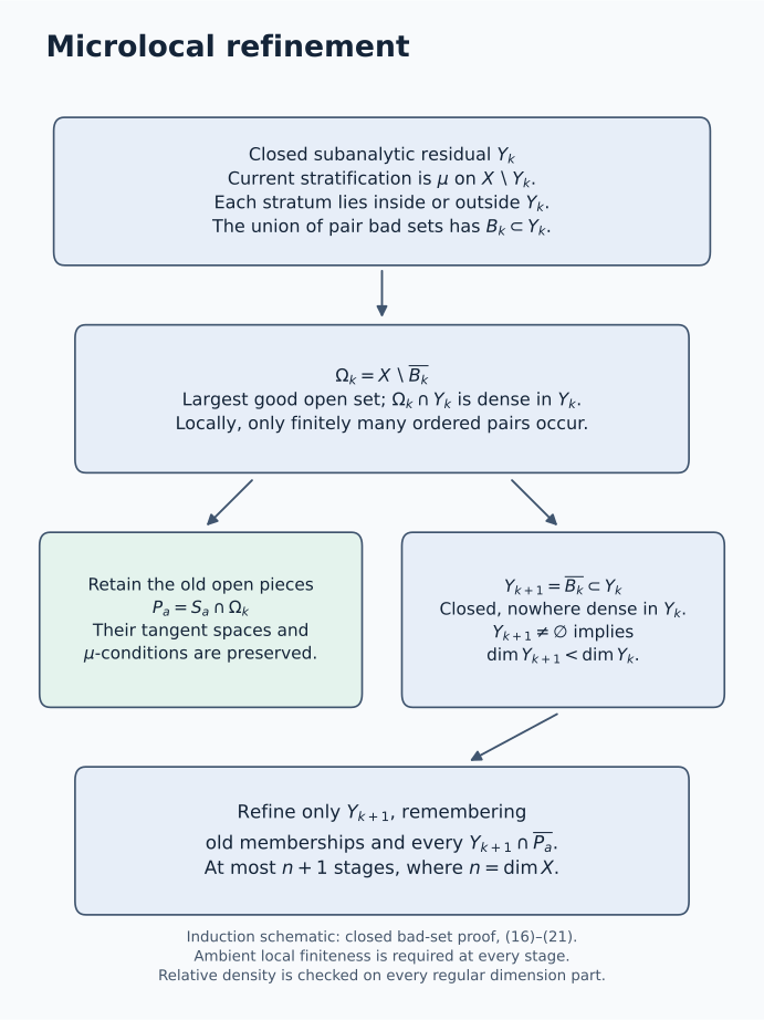
Induction schematic. At stage $k$, the sets $Y_k$, $B_k$ and $\Omega_k$ are the current residual, pair bad set and largest good open set. Formulas (16) and (19) give $Y_{k+1}=\overline{B_k}$, (20) supplies strict dimension decrease, and (21) retains the existing strata on $\Omega_k$. The refinement inside $Y_{k+1}$ remembers every upper closure. The proof above checks density on every regular dimension part and all frontier incidences; ambient local finiteness is required throughout.

A μ-stratification carrying an isotropic cotangent set

Conormal-cover corollary. If $\Lambda\subset T^*X$ is closed, conic, subanalytic and isotropic, there is a μ-stratification $\mathcal S$ of $X$ such that

$$\Lambda\subset\Lambda_{\mathcal S}. \qquad\text{(22)}$$

Proof. The finite conormal-closure theorem gives subanalytic analytic bases $G_1,\ldots,G_m$ with

$$\Lambda\subset\bigcup_{i=1}^m\overline{T_{G_i}^*X}. \qquad\text{(23)}$$

Use the μ-refinement theorem with the finite cover consisting of all $G_i$ and $X\setminus\bigcup_iG_i$, and retain compatibility (1). Every stratum that meets a $G_i$ is then contained in it. The smooth inclusion $S_a\subset G_i$ gives

$$T_{G_i}^*X|_{S_a}\subset T_{S_a}^*X. \qquad\text{(24)}$$

Therefore every $T_{G_i}^*X$ lies in $\Lambda_{\mathcal S}$. This latter set is closed by (9), so it also contains their closures. Equations (23)–(24) prove (22). The bars in (23) have been accounted for through the closed total conormal set, rather than dropped from the finite cover. $\square$

The inclusion in (22) may be strict. A singular base point can require a full point-stratum conormal even when $\Lambda$ retains only a few limiting normal lines there.

Exercises with complete solutions

The order of a μ-pair

Difficulty: Introductory.

In $X=\mathbb R$, compare $(M,N)=(\mathbb R,\{0\})$ and $(M,N)=(\{0\},\mathbb R)$. Determine the neighborhood-good locus in the second target base.

Solution. The conormal to $\mathbb R$ is its zero section, while the conormal to $\{0\}$ is the whole vertical fibre. The sum is symmetric, and its full limiting value is that vertical fibre at zero: the base of the point conormal is always zero, both bases must tend to zero, and the covector on the zero section is zero. Every finite covector on the fibre can be realized with both bases equal to zero.

For the first ordered pair, the target conormal is the whole vertical fibre, so the condition holds. For the second, the target is the zero section, and any nonzero covector at zero violates it. Thus $B_{\{0\},\mathbb R}=\{0\}$, and $Q_{\{0\},\mathbb R}=\mathbb R\setminus\{0\}$. This is open dense in the target base. The example concerns the pair condition; its two bases are not disjoint strata of a partition.

Membership cells still need their boundary strata

Difficulty: Intermediate.

Use the cover $E_1=(-\infty,1]$, $E_2=[0,\infty)$ of $\mathbb R$. Compute its membership cells, carry out the ordinary refinement, and check all nontrivial frontier incidences.

Solution. The cells with membership indices $\{1\}$, $\{1,2\}$, $\{2\}$ are respectively

$$(-\infty,0),\qquad [0,1],\qquad (1,\infty). \qquad\text{(25)}$$

The middle cell is not an analytic submanifold at its endpoints. The regular top-dimensional interiors give $(-\infty,0)$, $(0,1)$, $(1,\infty)$, leaving $R=\{0,1\}$. Its refinement compatible with the upper frontiers gives the two point strata. The closure of the first interval meets only the point stratum $\{0\}$; that of the middle interval meets both point strata; that of the last meets only $\{1\}$. Every meeting includes the whole point stratum, so (2) holds. No distinct open intervals meet each other’s closures inside another interval. The five strata retain all original memberships.

They also form a μ-stratification. Each upper interval is open in $\mathbb R$, and each lower point has full cotangent conormal, so all incident pairs satisfy (5).

A smooth partition with a microlocal bad point

Difficulty: Advanced.

In $X=\mathbb R^3$, with coordinates $(x,y,z)$, put

$$F=\{x^3=y^3z\},\quad M=F\cap\{y\ne0\},\quad N=\{x=y=0\},\quad O=X\setminus F. \qquad\text{(26)}$$

Show that $(O,M,N)$ is an ordinary subanalytic stratification. Compute the bad locus of $(M,N)$, and give a compatible μ-refinement.

Solution. All these sets are semianalytic, hence subanalytic. The set $O$ is open. The parametrization

$$(s,t)\longmapsto(st,s,t^3),\qquad s\ne0, \qquad\text{(27)}$$

is an analytic embedding onto $M$, with analytic inverse $s=y,t=x/y$. Its tangent vectors are $(t,1,0)$ and $(s,0,3t^2)$; they are independent even at $t=0$, since $s\ne0$. Thus $M$ is a two-dimensional submanifold. The line $N$ is closed. The polynomial defining $F$ has a zero set with empty interior, so $\overline O=X$. Also $\overline M=F$: the points of $N$ are obtained by letting $s\to0$ with $t$ the real cube root of the prescribed $z$. Hence each frontier incidence includes the whole lower stratum, proving (2).

Write a conormal to $M$ as $a\,dx+b\,dy+c\,dz$. From the two tangent vectors,

$$b=-at,\qquad as+3t^2c=0. \qquad\text{(28)}$$

The conormal to $N$ consists of $a\,dx+b\,dy$, with zero $dz$ component. At $z_0\ne0$, a sequence on $M$ approaching $(0,0,z_0)$ has $t_j\to t_0\ne0$. In (6), the distance from $(s_jt_j,s_j,t_j^3)$ to any point of $N$ is at least $|s_j|$, and the conormal norm is at least $|a_j|$. The product condition forces $s_ja_j\to0$. Equation (28) then gives $c_j\to0$. Since the conormal on $N$ has zero $dz$ component, the limiting sum has zero $dz$ component as required. Thus the pair is good over every $z_0\ne0$.

At the origin, take $t_j=0$, $s_j\to0$ nonzero. The fixed covector $dz$ is conormal to $M$ by (28). Take the second base to be the origin and the second covector to be zero. The distance product tends to zero, while the sum remains $dz$, which is not conormal to $N$. Therefore the exact bad locus is the origin. Its neighborhood-good locus is $N\setminus\{0\}$.

The partition $(O,M,N\setminus\{0\},\{0\})$ is a μ-stratification. The pair from $M$ to the punctured line is good by the calculation; pairs from $O$ are good because it is open; every pair to the point is good because its conormal is the whole fibre. The frontier rule follows from $\overline{N\setminus\{0\}}=N$ and the previously computed closures. The punctured line may be kept as one disconnected stratum or split into two components.

Refinement can introduce a new μ-failure

Difficulty: Intermediate.

Explain why one cannot replace (21) by an arbitrary ordinary refinement of all of $X$, even when the old stratification is already μ. Give an explicit example using (26).

Solution. The one-stratum partition $\{\mathbb R^3\}$ is μ: there are no distinct incident pairs, and its total conormal is the zero section. The ordinary partition $(O,M,N)$ of (26) refines it, but the preceding solution exhibits a μ-failure at the origin. Thus ordinary refinement does not in general preserve the μ-condition.

In the induction, the pieces $P_a=S_a\cap\Omega$ retain the tangent spaces of their parent strata. Restricting to an open set preserves their limiting-sum conditions by locality. Only the residual closed set is repartitioned; its new pair conditions are addressed at the next induction step. This is why the already-good open part survives.

A locally finite union with infinitely many strata

Difficulty: Intermediate.

Stratify $\mathbb R$ by the intervals $(m,m+1)$ and the points $\{m\}$, for all $m\in\mathbb Z$. Compute its total conormal set and verify the μ-condition and closedness directly. Does the dimension bound on the construction force finitely many global strata?

Solution. A bounded base neighborhood meets only finitely many intervals and integers, so the partition is locally finite. Its frontier incidences are the endpoints of each interval, and the condition holds for each such pair because the upper interval is open and the lower stratum is a point. The total conormal is

$$\Lambda_{\mathcal S} =\{(x;\xi):\xi=0\} \cup\bigcup_{m\in\mathbb Z}\{(m;\xi):\xi\in\mathbb R\}. \qquad\text{(29)}$$

It is conic. Near any base point it is a finite union of closed analytic lines, so it is subanalytic and isotropic. It is closed: a convergent sequence of integer base coordinates is eventually confined to a finite set, so after passage to a subsequence that base is a fixed integer; zero-section limits stay on the zero section. The family has infinitely many global strata. A bound on the number of dimension-induction stages gives no bound on that global number.

The lower refinement must remember an upper closure

Difficulty: Intermediate.

In $\mathbb R^2$, let $Y'$ be the horizontal axis and let the already chosen outside strata include

$$P=\{x>0,y>0\},\quad Q=\{x<0,y>0\},\quad R=\{x=0,y>0\},\quad H=\{y<0\}. \qquad\text{(30)}$$

Why does adding the whole axis as a single lower stratum fail the frontier rule? Give a compatible lower refinement and check its incidences with these upper pieces.

Solution. The closure of $P$ meets the axis in $\{(x,0):x\ge0\}$, which is nonempty but does not contain the whole axis. Thus one lower stratum equal to the entire axis would violate (2).

Refine the axis into its positive half, its negative half and the origin. The closure of $P$ contains the positive half and the origin and misses the negative half. The closure of $Q$ contains the negative half and the origin and misses the positive half. The closure of $R$ meets the axis only at the origin. The closure of $H$ contains all three lower strata. Every lower piece lies wholly in or wholly outside each of these closures, exactly as imposed in (12) and (21). Inside the lower family, each half-axis has the origin as its only additional frontier. Inside the outside family, $R$ is in the closures of $P,Q$, and there are no partial incidences. The combined partition is an ordinary stratification.

A conormal cover can enlarge a singular fibre

Difficulty: Advanced.

For $G=\{(t^2,t^3):t\ne0\}\subset\mathbb R^2$, let $\Lambda=\overline{T_G^*\mathbb R^2}$. Explain how (22) covers the origin fibre. Determine that fibre and compare it with the point-stratum conormal. Prove that a closed subanalytic bad set loses dimension even when the ambient closed set has components of different dimensions.

Solution. Writing a covector as $a\,dx+b\,dy$, annihilation of $(2t,3t^2)$ gives $2a+3tb=0$. A finite covector limit at the origin therefore has $a=0$, while every finite $b$ occurs. Thus $\Lambda$ has only the line $\mathbb R\,dy$ at the origin. A compatible μ-stratification may have the origin as a point stratum; its conormal there is the full two-dimensional cotangent fibre and contains the limiting line. This illustrates the inclusion, rather than equality, in (22). In its proof, closure of the total stratum conormal is what covers the limit from $G$.

For the dimension assertion, let $D\subset Y$ be closed, subanalytic and nowhere dense in the closed subanalytic $Y$, and put $d=\dim Y$. On each dimension-$d$ regular part of $Y$, a dimension-$d$ regular piece of $D$ would be an open subset, contradicting nowhere density. Thus its dimension is at most $d-1$ there. The singular part of $Y$ and all smaller-dimensional regular parts already have dimension at most $d-1$. The finite dimensional decomposition and local finite-union rule give $\dim D\le d-1$. Lower-dimensional subsets can remain in $D$; no nonempty relatively open part of $Y$ can remain in it. This is compatible with the density proof above, which also treats smaller regular components rather than assuming a pure-dimensional $Y$.

A tangential approach can still have a bad weighted witness

Difficulty: Intermediate.

In $\mathbb R^2$, let $M=\{(s,s^2):s>0\}$ and $N=\{(u,0):u\in\mathbb R\}$. Test the μ-condition at the origin using both (W2) and the limiting covectors. Explain what changes if the lower base is the single point $\{0\}$.

Solution. At $x_s=(s,s^2)$, a unit tangent is $(1,2s)/\sqrt{1+4s^2}$. With $y_s=(s,0)$, the unit normal has first component of magnitude $2s/\sqrt{1+4s^2}$. Thus

$$\frac{e(x_s,y_s)}{|x_s-y_s|} =\frac{2}{s\sqrt{1+4s^2}}\longrightarrow+\infty. \qquad\text{(W5)}$$

The estimate (W2) fails. Directly choose $\xi_s=-dx+(2s)^{-1}dy$ at $x_s$ and $\eta_s=-(2s)^{-1}dy$ at $y_s$. The first annihilates $(1,2s)$, the second annihilates the horizontal axis, their sum is $-dx$, and

$$|x_s-y_s|\,|\xi_s| =s^2\sqrt{1+(2s)^{-2}}\longrightarrow0. \qquad\text{(W6)}$$

Their limit is not conormal to $N$. Nevertheless the ordinary tangent lines of $M$ converge to the tangent line of $N$: that convergence alone misses the rate measured by (W5). These two whole bases do not satisfy the frontier rule, since the closure of $M$ meets $N$ only at the origin. Splitting the lower base there makes the approaching target a point, whose conormal is the whole cotangent fibre; the μ-condition for that ordered pair then holds. The calculation tests the condition for a pair without assuming it already belongs to a stratification.

What the construction supplies

We now have both a closed total conormal set attached to a μ-stratification and a compatible μ-stratification attached to a closed subanalytic isotropic cotangent set. The next steps distinguish conormal directions that are shared by several strata, organize strata into dimension filtrations, and produce generic squared-distance functions with transverse cotangent intersections. These will connect the geometry to constructibility and Morse calculations.

For the underlying subanalytic geometry, see Bierstone and Milman, Semianalytic and subanalytic sets. Kashiwara and Schapira’s Microlocal Study of Sheaves develops the isotropic-conormal setting. Trotman’s paper supplies the metric equivalence; the construction here proceeds through the full limiting-sum isotropy theorem, the generic-base argument, and the explicit induction on the dimension of the closed bad set. The analytic critical-value theorem used for generic bases is proved in Finite conormal closures and generic base directions. The underlying subanalytic regularity and dimension results, the analytic-calculus inputs and the singular-form and uniformization foundations of the full limiting-sum theorem are used as prerequisites.