Changing an interior frame to extend an invertible matrix

The construction below supplies the matrix extension needed when an elliptic problem has already become multiplication by an invertible matrix outside a compact set. Its input matrix can have singular behavior at that compact set and at the boundary of its open domain. A change of frame on the whole open domain carries that behavior into an invertible matrix on the exterior. The multiplication order is retained throughout.

The proof here uses a directly constructed connection and a convergent matrix integral series. It does not assume a theorem asserting triviality of bundles over a contractible base.

1. Statement, types, and elementary inputs

Let $\nu,N$ be positive integers. Let $U\subset\mathbb R^\nu$ be bounded and open, let $K\subset U$ be compact, and let $$a:U\setminus K\longrightarrow \operatorname{GL}(N,\mathbb C) \tag{M1}$$ be smooth. There are smooth maps $$A_0:U\longrightarrow\operatorname{GL}(N,\mathbb C), \qquad A_\infty:\mathbb R^\nu\setminus K\longrightarrow \operatorname{GL}(N,\mathbb C) \tag{M2}$$ such that $$A_\infty(x)=a(x)A_0(x) \quad(x\in U\setminus K). \tag{M3}$$ For some $R>0$, the exterior factor additionally satisfies $$A_\infty(x)=A_\infty(2R x/|x|) \quad(|x|\geq2R). \tag{M4}$$ Thus it is homogeneous of degree zero near infinity. No extension of $a$ across $K$ is required. No regularity of $\partial U$ or of $K$, connectedness of $U$, or uniform bounds on derivatives of $a$ near either omitted boundary are assumed.

We use finite matrix algebra, Euclidean compactness, ordinary differentiation and integration on compact intervals, smooth compact cutoffs, and uniform convergence of a series together with its derivatives. In particular, the scalar exponential series converges, and termwise differentiation and integration are valid when the differentiated series converge uniformly on the compact set concerned. The matrix transport equation needed here is proved in Section 2. The vector bundle, its smooth structure, its connection and its trivializing frame are constructed below.

The earlier finite matrix foundation, Sections 10.1–10.4 and 10.6, proves the coordinate maps, rank-nullity argument, determinant inverse and the operator-norm product bound used here. The metric and calculus foundation, Sections 12.3–12.8, 13.3–13.7, 13.10 and 14.4, proves compactness, compact extrema, countable coordinate bases, oriented integration, the full product and chain rules, smooth cutoffs and differentiation of uniformly convergent derivative series. The needed parameter version follows by applying the coordinate-segment identity (GC9) to each derivative on a compact coordinate box. Thus these elementary inputs have operative proofs in the course. The construction below still supplies its own ordered matrix equation, bundle charts and frame.

Choose a real $\psi\in C_c^\infty(U)$ with $0\leq\psi\leq1$ and $\psi=1$ on an open neighborhood $W$ of $K$. Here and below a compactly supported function on $U$ is extended by zero to $\mathbb R^\nu$. For completeness, choose finitely many balls whose smaller concentric balls cover $K$ and whose closed larger balls lie in $U$. Choose a smooth cutoff $b_j$ supported in each larger ball and equal to one on its smaller ball. Then $$\psi=1-\prod_j(1-b_j) \tag{M5}$$ has the stated properties. If $K$ is empty take $\psi=0$; the neighborhood condition is then vacuous. The finite ball cover follows from compactness of $K$ and openness of $U$, and it does not require any boundary regularity.

2. A matrix transport equation with smooth parameters

Let $[b,c]$ be a compact interval, let $Z\subset\mathbb R^d$ be open, and let $B(t,z)$ be a smooth $N\times N$ complex matrix on a neighborhood of $[b,c]\times Z$. Consider $$\partial_t Q(t,z)=B(t,z)Q(t,z),\qquad Q(b,z)=I_N. \tag{M6}$$ For $b\leq t\leq c$, put $$Q(t,z)=I_N+\sum_{k=1}^{\infty} \int_{b\leq t_k\leq\cdots\leq t_1\leq t} B(t_1,z)B(t_2,z)\cdots B(t_k,z) \,dt_k\cdots dt_1. \tag{M7}$$ The order of the matrix factors in this formula is part of the definition. Use the operator norm induced by the standard Hermitian norm on $\mathbb C^N$; it satisfies $\|ST\|\leq\|S\|\|T\|$, since $\|STv\|\leq\|S\|\|T\|\|v\|$ for every vector $v$. On a compact parameter set $L\Subset Z$, set $M_0=\sup\|B(t,z)\|$. The norm of its $k$-th term is at most $$\frac{M_0^k(c-b)^k}{k!}. \tag{M8}$$ Indeed the integration simplex has volume $(t-b)^k/k!$, as follows by successively integrating the constant function one. The exponential series therefore gives locally uniform convergence.

Here is the derivative assertion used below, including its quantitative justification. Fix a parameter multiindex $\alpha$ of length $r$, and choose $M_r\geq1$ bounding every $\partial_z^\beta B$, $|\beta|\leq r$, on $[b,c]\times L$. Apply the $r$ coordinate derivatives successively to the product of $k$ factors. There are at most $k^r$ resulting terms if repetitions are counted; each term is a product of $k$ matrices whose norms are at most $M_r$. Thus the differentiated integral has norm at most $$\frac{k^r M_r^k(c-b)^k}{k!}. \tag{M9}$$ This series converges by the ratio test. It proves locally uniform convergence of every parameter derivative and validates differentiation under all the integrals and their sum. Differentiation of the outer upper endpoint in (M7) gives (M6), because the first matrix becomes $B(t,z)$ and the remaining ordered integral is the preceding term. The equation then gives all mixed time and parameter derivatives inductively. Consequently $Q$ is smooth.

There is uniqueness with any prescribed initial matrix. The difference $D$ of two solutions with the same initial matrix satisfies $D(t)=\int_b^t B(s)D(s)\,ds$. Iterating this identity $k$ times and bounding $D$ on the compact interval gives $$\|D(t)\|\leq \sup_{[b,c]}\|D\| \frac{M_0^k(c-b)^k}{k!}. \tag{M10}$$ The right side tends to zero, so $D=0$.

The equation $\partial_t T=-TB$, $T(b)=I_N$, has a smooth solution by the same series argument with multiplication on the right. Differentiating yields $\partial_t(TQ)=0$; hence $TQ=I_N$. Square finite matrices with a left inverse are invertible, so $$Q(t,z)^{-1}=T(t,z). \tag{M11}$$

The inverse has an ordered series too. In the same original interval and parameters, its complete formula is $$T(t,z)=I_N+\sum_{k=1}^{\infty}(-1)^k \int_{b\leq t_k\leq\cdots\leq t_1\leq t} B(t_k,z)B(t_{k-1},z)\cdots B(t_1,z) \,dt_k\cdots dt_1. \tag{MT1}$$ Each product has the reverse order from (M7), and each term retains its sign. The integral estimates (M8)–(M9) apply to this series in that order. Differentiating its outer endpoint gives $T_k'(t,z)=-T_{k-1}(t,z)B(t,z)$: the new endpoint factor is the rightmost one. Summing gives $T'=-TB$, including the initial value $T(b,z)=I_N$. This supplies the right-multiplication construction used in (M11).

Here is the full parameter product rule behind (M9). Write a multiindex derivative as a labelled list $D_1\cdots D_r$, retaining a repeated label direction whenever it occurs. For $k\geq1$, $$D_1\cdots D_r[B(t_1,z)\cdots B(t_k,z)] =\sum_{\sigma:\{1,\ldots,r\}\to\{1,\ldots,k\}} (D_{\sigma^{-1}(1)}B)(t_1,z)\cdots (D_{\sigma^{-1}(k)}B)(t_k,z). \tag{MT2}$$ Within each sublist the original derivative order is kept; an empty sublist means the undifferentiated factor. The sum has exactly $k^r$ labelled assignments, including repeated identical terms when the directions coincide. Applying one new derivative appends its label to precisely one factor, which proves the formula by induction. The same rule applies to (MT1) with its reversed factor list. On a compact parameter box the bound (M9) holds for every assignment sum. The partial sums and all their derivatives therefore converge uniformly there. Passing to the limit in (GC9), first at order zero and then on each already retained derivative, proves that these limits are the actual parameter derivatives. It also justifies passing each derivative under a fixed simplex integral. Differentiating (M6) or $T'=-TB$ then gives every mixed time and parameter derivative.

For the actual endpoint continuation, use the nested oriented integral from $b$ to $t$, then from $b$ to the first integration variable, and so on. When $t<b$, its $k$-th term for $Q$ is exactly $$(-1)^k\int_{t\leq t_1\leq\cdots\leq t_k\leq b} B(t_1,z)\cdots B(t_k,z)\,dt_k\cdots dt_1. \tag{MT3}$$ Reversing the $k$ original limits supplies the $k$ signs and the displayed ordering. Its derivative assignment sum has bound $k^r M_r^k|t-b|^k/k!$, by the same full product rule and the nonnegative simplex volume. For $T$ retain both the coefficient $(-1)^k$ of (MT1) and the $k$ orientation signs, with the reversed product. Thus both continued series and every derivative converge uniformly on each compact interval within the coefficient’s original neighborhood. Their nested integral recursions still give $Q'=BQ$, $T'=-TB$ and the same initial values. Uniqueness makes their restrictions agree with the original solutions on $[b,c]$. The coefficient neighborhood permits this continuation locally in the parameters beyond both time endpoints. It proves the asserted endpoint smoothness with every factor and sign retained. In particular the solution never leaves $\operatorname{GL}(N,\mathbb C)$. The solution from time $s$ to time $t$ is $Q(t,z)Q(s,z)^{-1}$, and its multiplication rule is $$\bigl(Q(t)Q(s)^{-1}\bigr) \bigl(Q(s)Q(r)^{-1}\bigr)=Q(t)Q(r)^{-1}. \tag{M12}$$ This proves both the subdivision rule and invertibility of transport, without a separate existence or parameter theorem for ordinary differential equations.

3. The two coordinate systems and their exact connection

Write $V=\mathbb R^\nu\setminus K$. It is open, and $U\cup V=\mathbb R^\nu$. Form a rank-$N$ bundle $E$ by taking the disjoint union of $U\times\mathbb C^N$ and $V\times\mathbb C^N$ and imposing the identifications $$(x,u)_U\sim(x,v)_V \quad\Longleftrightarrow\quad v=a(x)u, \qquad x\in U\cap V. \tag{M13}$$ The reverse identification is $u=a(x)^{-1}v$. Inversion is smooth, since matrix inversion is the adjugate divided by the nonvanishing determinant. These identifications define two genuine local trivializations: every equivalence class over $U$ has a unique $U$-coordinate, and similarly over $V$. The chart transition on the overlap is the smooth diffeomorphism $(x,u)\mapsto(x,a(x)u)$, with the displayed inverse. Their quotient topology makes each trivialization an open chart. The total space is Hausdorff: different base points are separated in the base, while two different vectors over the same point are separated in one of these common local charts. It is second countable because each of its two open charts is a Euclidean open subset and the union of their two countable bases is a countable base for the total space. These observations verify the smooth vector bundle structure directly.

Define matrix-valued one-forms in its two charts by $$\omega_U=(1-\psi)a^{-1}\,da \quad\hbox{on }U\setminus K, \qquad \omega_V=-\psi\,(da)a^{-1} \quad\hbox{on }U\cap V. \tag{M14}$$ Extend $\omega_U$ by zero on $W$, and extend $\omega_V$ by zero on $V\setminus\operatorname{supp}\psi$. Both extensions are smooth. For the first extension the prefactor $1-\psi$ is identically zero on the open set $W$; no value or bound for $a$ at $K$ is used. For the second, the support of $\psi$ is a compact subset of $U$, so the formula is identically zero on a neighborhood of every point outside that support. On the overlaps of each definition the formulas agree. The possible unboundedness of $a$ or $a^{-1}$ near $K$ or $\partial U$ therefore creates no extension problem.

For every $x\in U\cap V$, direct multiplication gives $$\begin{aligned} a\omega_Ua^{-1}-(da)a^{-1} &=(1-\psi)(da)a^{-1}-(da)a^{-1}\\ &=-\psi(da)a^{-1}=\omega_V. \end{aligned} \tag{M15}$$ In particular, if a section has coordinates $u,v=a u$, then $$dv+\omega_Vv=a(du+\omega_Uu). \tag{M16}$$ This equality proves that the two formulas $d+\omega_U$ and $d+\omega_V$ define a connection on the original bundle. It also records its exact relation to the transition matrix; none of the matrices in (M14) have been commuted.

For a smooth path $\gamma$ lying in one chart, call a vector field along it parallel when its coordinate $f(t)$ satisfies $$f'(t)=-\omega_i(\gamma(t))[\gamma'(t)]f(t), \qquad i=U\hbox{ or }V. \tag{M17}$$ This is the equation of Section 2. If $\gamma$ lies in both charts and $v(t)=a(\gamma(t))u(t)$, differentiation gives $$\begin{aligned} v'(t) &=(da)(\gamma(t))[\gamma'(t)]u(t) -a(\gamma(t))\omega_U(\gamma(t))[\gamma'(t)]u(t)\\ &=-\omega_V(\gamma(t))[\gamma'(t)]v(t). \end{aligned} \tag{M18}$$ The second equality is precisely (M15). Therefore parallel transport in either chart describes the same linear map between the original fibers of $E$.

4. A smooth frame from all radial paths

Choose any linear isomorphism $e:\mathbb C^N\to E_0$, and for every $x\in\mathbb R^\nu$ use the path $$\gamma_x(t)=tx,\qquad0\leq t\leq1. \tag{M19}$$ Parallel transport along it defines an isomorphism $$F(x):\mathbb C^N\longrightarrow E_x. \tag{M20}$$ We verify existence, independence of the chart subdivisions, and smoothness of this family.

Fix an endpoint $x_*$. The inverse images $\gamma_{x_*}^{-1}(U)$, $\gamma_{x_*}^{-1}(V)$ are an open cover of the compact interval $[0,1]$. There is a finite subdivision $0=t_0<t_1<\cdots<t_\ell=1$ for which each closed segment $\gamma_{x_*}([t_{j-1},t_j])$ is contained in one of the two charts, denoted $O_j$. One elementary justification of the needed subdivision is to take a finite subcover of small intervals with closures in the original inverse images and then choose a sufficiently fine uniform subdivision. Equivalently, a finite open cover of a compact interval has a positive Lebesgue number: if no such number existed, a sequence of subsets of diameters tending to zero but contained in no cover member would have a subsequence accumulating at one point, contradicting openness of a cover member at that point.

The compact segment in each open $O_j$ has positive distance from its closed complement whenever that complement is nonempty. Since $|tx-tx_*|\leq|x-x_*|$, an endpoint neighborhood $Z$ of $x_*$ can be chosen so that $$\gamma_x([t_{j-1},t_j])\subset O_j \quad(x\in Z,\ 1\leq j\leq\ell). \tag{M21}$$ If a complement is empty there is no restriction from that segment. At each subdivision endpoint both adjacent charts contain the endpoint, including for every $x\in Z$. The same finite itinerary therefore works for the whole endpoint neighborhood.

On segment $j$ set $$B_j(t,x)=-\omega_{O_j}(tx)[x]. \tag{M22}$$ This is smooth on a neighborhood of $[t_{j-1},t_j]\times Z$, after shrinking $Z$ when needed. Section 2 gives its smooth invertible transport matrix $Q_j(x)$ from $t_{j-1}$ to $t_j$. Between consecutive segments insert the exact coordinate transition $$g_{j+1,j}(x)= \begin{cases} a(t_jx),&O_j=U,\ O_{j+1}=V,\\ a(t_jx)^{-1},&O_j=V,\ O_{j+1}=U,\\ I_N,&O_j=O_{j+1}. \end{cases} \tag{M23}$$ If $C_0$ is the coordinate matrix of $e$ in the first chart at the fixed origin, the coordinate matrix of (M20) in the final chart is $$Q_\ell(x)g_{\ell,\ell-1}(x)Q_{\ell-1}(x) \cdots g_{2,1}(x)Q_1(x)C_0. \tag{M24}$$ For one segment this expression means $Q_1(x)C_0$. Every matrix factor is invertible and smooth. Inserting a subdivision inside a single chart leaves (M24) unchanged by (M12). Changing the chart on a segment contained in the overlap leaves it unchanged by (M18) and uniqueness in Section 2. Any two finite itineraries have a common refinement. On each refined segment either their chart names agree or the path lies in both charts; these two observations consequently prove that (M24) is independent of all subdivision and chart choices. They also show that changing the chart used at the origin merely replaces $C_0$ by the coordinate matrix of the same fixed $e$, with the compensating transition, so the map (M20) is well defined in the original fibers.

Formula (M24) proves smoothness on $Z$ in its final chart. If another chart is desired at an endpoint in the overlap, multiplication by $a(x)$ or $a(x)^{-1}$ gives its smooth coordinates there. Since $x_*$ was arbitrary, $F$ is a global smooth frame. Its inverse is smooth in each chart by finite matrix inversion, and it is an isomorphism $\mathbb R^\nu\times\mathbb C^N\to E$ over the identity of the base.

Let $F_U:U\to\operatorname{GL}(N,\mathbb C)$ and $F_V:V\to\operatorname{GL}(N,\mathbb C)$ be its two coordinate matrices. Applying the defining identification (M13) to every column of the same frame gives the exact identity $$F_V(x)=a(x)F_U(x) \quad(x\in U\setminus K). \tag{M25}$$ This is an explicit isomorphism, not an appeal to a classification of bundles. Arbitrarily many components of $U$ and irregularities of $K$ have not changed the construction: each individual radial path uses only a finite cover of a compact interval.

What radial transport does to the original connection

The frame $F$ trivializes the original bundle. The connection in this frame need not vanish in every direction. In the two original charts put $$\Xi_U=F_U^{-1}dF_U+F_U^{-1}\omega_UF_U,\qquad \Xi_V=F_V^{-1}dF_V+F_V^{-1}\omega_VF_V. \tag{MF1}$$ These are one-forms on $U$ and $V$, respectively. Using $F_V=aF_U$, $dF_V=(da)F_U+a\,dF_U$ and (M15), their overlap comparison is $$\begin{aligned} \Xi_V &=F_U^{-1}a^{-1}(da)F_U+F_U^{-1}dF_U +F_U^{-1}a^{-1}\bigl[a\omega_Ua^{-1}-(da)a^{-1}\bigr]aF_U\\ &=F_U^{-1}dF_U+F_U^{-1}\omega_UF_U=\Xi_U. \end{aligned} \tag{MF2}$$ Both derivative-of-transition contributions are displayed before their cancellation. Hence (MF1) gives one smooth matrix-valued one-form $\Xi$ on the entire original $\mathbb R^\nu$.

For any fixed $x$ and $0<t\leq1$, the radial path to $tx$ is the path to $x$ stopped at time $t$, with a linear reparametrization. Substitution in the segment equation (M17), followed by uniqueness and the subdivision identity, proves $F(tx)=P_{0,t}^{\gamma_x}e$, where $P_{0,t}^{\gamma_x}:E_0\to E_{tx}$ is that very transport. In a chart about $x$, differentiation at $t=1$ gives $$dF_i(x)[x]=-\omega_i(x)[x]F_i(x),\qquad \Xi(x)[x]=0. \tag{MF3}$$ For the left derivative at one, continuity extends the equation to the endpoint; the same radial construction on a slightly longer ray supplies its two-sided derivative. At $x=0$ the evaluated direction is zero, so (MF3) holds there as well. This is the exact property of the transported frame. It is sufficient for its construction and makes no assertion about transport along other paths.

The retained cutoff also lets us compute what prevents such an assertion. For matrix one-forms define $(\alpha\wedge\beta)(X,Y)=\alpha(X)\beta(Y)-\alpha(Y)\beta(X)$, with the displayed product order. On $U\setminus K$ put $\theta=a^{-1}da$, and on the overlap put $\phi=(da)a^{-1}$. Differentiating $a^{-1}a=I_N$ gives $d(a^{-1})=-a^{-1}(da)a^{-1}$. Applying the ordinary coordinate product rules to these one-forms gives $d\theta=-\theta\wedge\theta$ and $d\phi=\phi\wedge\phi$. Consequently the curvature forms $\Omega_i=d\omega_i+\omega_i\wedge\omega_i$ are $$\begin{aligned} \Omega_U&=-d\psi\wedge\theta -\psi(1-\psi)\theta\wedge\theta,\\ \Omega_V&=-d\psi\wedge\phi -\psi(1-\psi)\phi\wedge\phi,\\ \Omega_V&=a\Omega_Ua^{-1}. \end{aligned} \tag{MF4}$$ For example, the first line follows by retaining $-d\psi\wedge\theta-(1-\psi)\theta\wedge\theta +(1-\psi)^2\theta\wedge\theta$; its last two coefficients have difference $-\psi(1-\psi)$. The second retains $-d\psi\wedge\phi-\psi\phi\wedge\phi+\psi^2\phi\wedge\phi$. The last equality uses $\phi=a\theta a^{-1}$, with $a^{-1}a$ cancelled only between adjacent factors. All forms extend by the same zero-neighborhood argument used for (M14). Their possible nonzero values lie in the transition region of the original cutoff. The exact coordinate comparison (MF2) and the radial identity (MF3) therefore do not require a flat connection.

5. Freeze the exterior radius while fixing the open domain

Choose $R>0$ with $\overline U\subset\{x:|x|<R\}$. Such a choice is possible because $U$ is bounded. Choose a smooth scalar function $\eta$ on $[0,\infty)$, with values in $[0,1]$, equal to zero for $r\leq R$ and equal to one for $r\geq2R$. Define $$\rho(r)=(1-\eta(r))r+2R\eta(r), \qquad h(x)= \begin{cases} x,&|x|\leq R,\\ \rho(|x|)x/|x|,&|x|>R. \end{cases} \tag{M26}$$ This is smooth on $\mathbb R^\nu$: the second formula agrees with the identity wherever $\eta=0$, and the identity defines it near the origin. For $r\geq R$, both $r$ and $2R$ are at least $R$, so their convex combination satisfies $\rho(r)\geq R$. Hence $h$ maps $V$ into $V$: inside the radius-$R$ ball it fixes every point, and outside it the image remains at radius at least $R$, which is disjoint from $K$. It fixes every point of $U$ and is equal to $2R x/|x|$ for $|x|\geq2R$.

Now set $$A_0(x)=F_U(x)\quad(x\in U), \qquad A_\infty(x)=F_V(h(x))\quad(x\in V). \tag{M27}$$ These maps have exactly the domains and codomains in (M2). Smoothness and invertibility follow from those of $F_U,F_V$ and the inclusion $h(V)\subset V$. For $x\in U\setminus K$, the equality $h(x)=x$ and (M25) give (M3) with its stated right factor. For $|x|\geq2R$, (M26) gives (M4). This proves the theorem.

The construction also gives explicit exterior symbol bounds. For every multiindex $\alpha$, there are finite constants $C_\alpha,D_\alpha$ such that $$\|\partial^\alpha A_\infty(x)\| \leq C_\alpha |x|^{-|\alpha|},\qquad \|\partial^\alpha A_\infty(x)^{-1}\| \leq D_\alpha |x|^{-|\alpha|} \quad(|x|\geq2R). \tag{M28}$$ To verify them without assuming estimates on the original $a$, extend the smooth angular matrix $F_V(2R\theta)$ by $H(x)=F_V(2Rx/|x|)$ for every $x\ne0$. For $t>0$, $H(tx)=H(x)$. Differentiating in $x$ gives $t^{|\alpha|}(\partial^\alpha H)(tx)=(\partial^\alpha H)(x)$. Taking $x=2R\theta$, $t=|y|/(2R)$, yields (M28) with $$C_\alpha=(2R)^{|\alpha|} \max_{|x|=2R}\|\partial^\alpha H(x)\|. \tag{M29}$$ For the inverse use $H^{-1}$, which is smooth by inversion and has the same homogeneity. Its maxima on that compact sphere are finite. Formula (M4) identifies $H$ and $A_\infty$, with every derivative, on the exterior, including its boundary by smoothness. These are exterior estimates; no bound near $K$ or $\partial U$ has been asserted.

If $U$ is empty, then $K$ is empty and the theorem holds by taking the empty $A_0$ and the constant identity for $A_\infty$. If zero-dimensional Euclidean space or rank zero is allowed, the same statement is immediate: the base is a single point in the first case, so the exterior condition is vacuous for positive $R$; in the second case every fiber map is the unique isomorphism of the zero vector space. These conventions do not impose restrictions on the positive-dimensional theorem.

6. An example and an explicit test of the factor order

Identify $\mathbb R^2$ with $\mathbb C$, take $U=\{z:|z|<2\}$, $K=\{0\}$, and put $$b(z)=\frac1{4-|z|^2},\qquad a(z)=e^{b(z)}\frac{z}{|z|}\quad(0<|z|<2). \tag{M30}$$ This is smooth and nonzero on precisely the required punctured domain. It has no continuous extension across the origin: as positive real $z\to0$, its limit is $e^{1/4}$, whereas on the negative real ray the limit is $-e^{1/4}$. Its norm also diverges on approaching the outer boundary. Nevertheless one may take $$A_0(z)=e^{-b(z)}\quad(|z|<2), \qquad A_\infty(z)=z/|z|\quad(z\ne0). \tag{M31}$$ The first function is smooth and strictly positive everywhere on its open domain, including at zero, although it tends to zero at its omitted outer boundary. The second is smooth, invertible and homogeneous of degree zero on its entire domain. Multiplying the displayed formulas proves (M3). This example verifies why neither an extension through $K$ nor uniform invertibility up to $\partial U$ may be inserted among the hypotheses.

Here is a matrix exercise with its solution. Suppose $(A_0,A_\infty)$ satisfies (M3) and $C\in\operatorname{GL}(N,\mathbb C)$ is constant. Determine a new pair representing the same $a$, and decide whether multiplication on the other side is valid. Right multiplication gives $$\widetilde A_0=A_0 C, \qquad \widetilde A_\infty=A_\infty C; \quad a\widetilde A_0=(aA_0)C=\widetilde A_\infty. \tag{M32}$$ All domains, invertibilities and exterior homogeneities are preserved. Left multiplication would instead require $a C A_0=C a A_0$, which, since $A_0$ is invertible, is equivalent to $aC=Ca$ at each point. For example take constant matrices $$a=\begin{pmatrix}1&1\\0&1\end{pmatrix},\qquad C=\begin{pmatrix}2&0\\0&1\end{pmatrix}. \tag{M33}$$ Their products are respectively $aC=\begin{pmatrix}2&1\\0&1\end{pmatrix}$ and $Ca=\begin{pmatrix}2&2\\0&1\end{pmatrix}$, so left multiplication fails. The pointwise identity in the theorem has a definite order even though its scalar example does not detect it.

A computed transport with a parameter

Baake and Schlägel’s The Peano–Baker series, Section 2 and the first example in Section 4, provide an accessible teaching comparison for (M7). Their scalar parameter called $a$ is called $\lambda$ here, to keep it distinct from the original transition function (M1). Every entry of their time-dependent matrix is retained: $$B_\lambda(t)=\begin{pmatrix}1&t\\0&\lambda\end{pmatrix}, \qquad t\in\mathbb R,\quad\lambda\in\mathbb C. \tag{MP1}$$ Complex parameters mean their two real coordinates for smoothness. Take initial time zero and retain the equation $Q'=B_\lambda Q$, $Q(0)=I_2$. For $n\geq1$ its ordered term is $$I_n(t,\lambda)= \begin{pmatrix} t^n/n!&t^{n+1}\alpha_n(\lambda)/(n+1)!\\ 0&(\lambda t)^n/n! \end{pmatrix},\qquad \alpha_n(\lambda)=\sum_{\ell=1}^n\ell\lambda^{\ell-1}. \tag{MP2}$$ This is a formula for every ordered term, rather than a truncation of the series. To prove it, at $n=1$ integrate (MP1) from zero to $t$. The recursion $I_{n+1}(t)=\int_0^tB_\lambda(s)I_n(s)\,ds$ keeps all four entries. The lower-left entry stays zero, and the two diagonal entries integrate to $t^{n+1}/(n+1)!$ and $(\lambda t)^{n+1}/(n+1)!$. The upper-right entry is $$\begin{aligned} \int_0^t\left[ \frac{s^{n+1}}{(n+1)!}\alpha_n(\lambda) +\frac{\lambda^n s^{n+1}}{n!}\right]ds &=\frac{t^{n+2}}{(n+2)!} \left[\alpha_n(\lambda)+(n+1)\lambda^n\right]\\ &=\frac{t^{n+2}}{(n+2)!}\alpha_{n+1}(\lambda). \end{aligned} \tag{MP3}$$ This proves the induction, including the oriented integrals when $t<0$.

The diagonal entries of the whole series are $e^t,e^{\lambda t}$. Its upper-right entry $f_\lambda$ has $f_\lambda'-f_\lambda=t e^{\lambda t}$ and $f_\lambda(0)=0$. Multiplying by the actual scalar inverse $e^{-t}$, applying the product rule and integrating the retained endpoints gives $$\begin{aligned} Q(t,\lambda)&=\begin{pmatrix}e^t&f_\lambda(t)\\0&e^{\lambda t}\end{pmatrix},\\ f_\lambda(t)&=e^t\int_0^t s e^{(\lambda-1)s}\,ds\\ &=\sum_{n=1}^{\infty} \frac{t^{n+1}}{(n+1)!}\sum_{\ell=1}^n\ell\lambda^{\ell-1},\\ f_\lambda(t)&= \frac{e^t-e^{\lambda t}-(1-\lambda)t e^{\lambda t}} {(1-\lambda)^2}\quad(\lambda\ne1),\\ f_1(t)&=\frac{t^2}{2}e^t. \end{aligned} \tag{MP4}$$ The quotient formula follows by integrating $s e^{(\lambda-1)s}$ as $e^{(\lambda-1)s}[s/(\lambda-1)-1/(\lambda-1)^2]$ and subtracting its value at zero. The integral formula remains defined at $\lambda=1$, where its integral is $t^2/2$. It also proves joint smoothness at that value: write it as $t^2e^t\int_0^1r e^{(\lambda-1)tr}\,dr$, and apply the compact-interval derivative proof with both real parameter coordinates. Thus neither the source parameter value nor its denominator has been dropped.

Exercise, with solution. Determine whether replacing the full ordered transport by the exponential of $\int_0^tB_\lambda(s)\,ds$ gives the same answer for every $\lambda$. The exact commutator is $$B_\lambda(t)B_\lambda(s)-B_\lambda(s)B_\lambda(t) =(1-\lambda)(s-t)\begin{pmatrix}0&1\\0&0\end{pmatrix}. \tag{MP5}$$ For a direct comparison, retain the full matrix integral $J(t,\lambda)=\begin{pmatrix}t&t^2/2\\0&\lambda t\end{pmatrix}$. In its actual matrix exponential series the upper-right entry of $J^m$, for $m\geq1$, is $(t^2/2)t^{m-1}\sum_{j=0}^{m-1}\lambda^j$. This follows by multiplying once by $J$ and retaining the diagonal and upper-right terms at each step. Hence $$\begin{aligned} (\exp J)_{12} &=\sum_{m=1}^{\infty} \frac{t^{m+1}}{2m!}\sum_{j=0}^{m-1}\lambda^j\\ &=\frac{t(e^t-e^{\lambda t})}{2(1-\lambda)}\quad(\lambda\ne1),\\ (\exp J(t,1))_{12}&=\frac{t^2}{2}e^t,\\ f_\lambda(t)-(\exp J)_{12} &=\frac{\lambda-1}{12}t^3+O(t^4)\quad(t\longrightarrow0). \end{aligned} \tag{MP6}$$ The last line follows from the exact third-order terms: $f_\lambda=t^2/2+(1+2\lambda)t^3/6+O(t^4)$, whereas $(\exp J)_{12}=t^2/2+(1+\lambda)t^3/4+O(t^4)$. Their remainders are bounded by the tails of the two convergent full series on every compact parameter set. For fixed $\lambda\ne1$ their third derivatives at zero differ by $(\lambda-1)/2$, proving that the two functions are not identical. At $\lambda=1$ all entries agree by the displayed formulas. This exercise explains why (M7) must keep its time and factor order even when an ordinary matrix exponential would be shorter to write.

7. Where the factors enter an index argument

This proves the factorization of arbitrary smooth invertible matrix data on $U\setminus K$, including its exact extension to the exterior and degree-zero behavior there. It supplies the matrix extension input to the later reduction of a manifold index problem to a Euclidean operator. The construction alone asserts no Fredholm property or equality of analytic indices for any operator. An operator index calculation additionally requires embedding, suspension, stable bundle trivialization, symbol and compact-kernel transport theorems. None of those is an assumption or conclusion of the factorization theorem proved here.

Choice dependence is concrete: selecting a different cutoff or initial frame produces other valid factors, while (M3) always preserves the same given matrix $a$.

The exact map between two choices of factors

Editorial consequence. Suppose $(A_0,A_\infty)$ and $(\widehat A_0,\widehat A_\infty)$ are two pairs satisfying (M2)–(M4) for the same original $U,K,a$, with their respective positive exterior radii. Define on the original cover $$G_U=A_0^{-1}\widehat A_0:U\to\operatorname{GL}(N,\mathbb C),\qquad G_V=A_\infty^{-1}\widehat A_\infty:V\to\operatorname{GL}(N,\mathbb C). \tag{MG1}$$ On $U\setminus K$, the original multiplication order proves $$G_V=(aA_0)^{-1}(a\widehat A_0) =A_0^{-1}a^{-1}a\widehat A_0 =A_0^{-1}\widehat A_0=G_U. \tag{MG2}$$ The two maps and their inverses are smooth and agree on the whole overlap. Since $U\cup V=\mathbb R^\nu$, they glue to a unique smooth invertible $G:\mathbb R^\nu\to\operatorname{GL}(N,\mathbb C)$. Its original restrictions give $$\widehat A_0=A_0G|_U,\qquad \widehat A_\infty=A_\infty G|_V. \tag{MG3}$$ Choose $S>0$ at least as large as both exterior threshold radii $2R$ and $2\widehat R$. Then each exterior factor depends only on its angular direction for $|x|\geq S$; evaluating each at $Sx/|x|$ gives $$G(x)=G(Sx/|x|)\quad(|x|\geq S). \tag{MG4}$$ Every exterior derivative of $G,G^{-1}$ has the same degree as in (M28), proved by differentiating (MG4) and taking compact-sphere maxima. On the remaining closed radius-$S$ ball, every derivative of these globally smooth maps has a finite maximum. In particular both $G$ and $G^{-1}$ are bounded on the entire original Euclidean space.

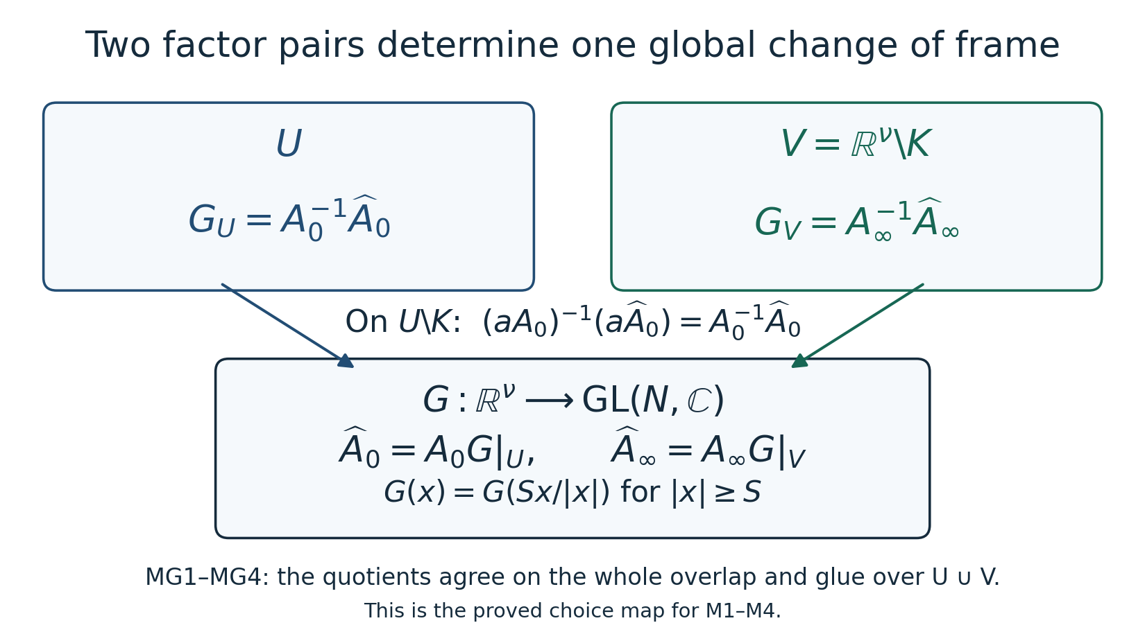
The diagram displays the exact map between two factor pairs for the same original transition. The quotient identities, global domain, inverse and exterior homogeneity are proved in (MG1)–(MG4). Its reproducible figure source is matrix-extension-choice-map.py.

Conversely, any smooth invertible $G$ on $\mathbb R^\nu$ homogeneous of degree zero near infinity gives a new valid pair by (MG3). The domains remain the original $U,V$, and $a(A_0G)=(aA_0)G=A_\infty G$. Outside one radius large enough for both maps their product and its inverse are homogeneous of degree zero. For two such maps the consecutive changes are $(A_0G)H=A_0(GH)$ and $(A_\infty G)H=A_\infty(GH)$, retaining their order. Thus the space of all valid factor pairs has a free transitive right action by the group of these global maps: existence of the connecting map is (MG1)–(MG4); uniqueness follows already from its two restrictions; and if a pair is unchanged, multiplication by its inverses gives $G=I_N$ on both cover members. A free transitive action means that any two pairs are related by precisely one group element. This is the complete mathematical content of choice dependence, and (M32) is its constant-map case.

For the jointly smooth families (M34)–(M38), the same calculation gives a jointly smooth global $G(x,z)$. If the two families each have a fixed exterior radius, then one common $S$ works for all $z$. On every compact $L\Subset Z$, compact-sphere and compact-ball maxima give all retained $x$- and $z$-derivative bounds for $G,G^{-1}$. There is no bound asserted over a noncompact parameter set. The parameter base need not itself be contractible: the initial fiber over $(0,z)$ already has the same chosen chart coordinates for every $z$.

The relation also preserves the precise compact-support maps needed in an operator application. Let $\mathcal D(U)=C_c^\infty(U;\mathbb C^N)$. Multiplication by $A_0$ is a bijection $\mathcal D(U)\to\mathcal D(U)$, inverse multiplication by $A_0^{-1}$, because both are smooth on the original open set. For any $u$, invertibility gives $A_0(x)u(x)=0$ if and only if $u(x)=0$, so the support is exactly unchanged. No bound at $\partial U$ is needed for this assertion. If $P:\mathcal D(U)\to\mathcal D(U)$ is a linear operator, then $$\begin{aligned} \ker(PA_0)&\longrightarrow\ker P,& u&\longmapsto A_0u,\\ \ker P&\longrightarrow\ker(PA_0),& v&\longmapsto A_0^{-1}v,\\ (PA_0)(\mathcal D(U))&=P(\mathcal D(U)),&&\\ \mathcal D(U)/(PA_0)(\mathcal D(U)) &\longrightarrow\mathcal D(U)/P(\mathcal D(U)),&[f]&\longmapsto[f] \end{aligned} \tag{MG5}$$ have the displayed domains, codomains and mutually inverse kernel maps; the quotient map is the identity on the identical range quotient. The kernel equality is verified by substitution in each direction, and the range equality uses the surjectivity of the multiplication map. If these two dimensions are finite, their actual difference is identical before and after the right composition. This proves the comparison used by the later Bott and Euclidean index reduction, Remark 13.2, without asserting its separate finiteness or Fredholm arguments here.

Smooth families on the original fixed domains

Editorial strengthening from the transport proof. Let $Z\subset\mathbb R^d$ be any open parameter set and retain the same bounded open $U$, compact $K\subset U$, and rank $N$. If $$a:(U\setminus K)\times Z\longrightarrow\operatorname{GL}(N,\mathbb C) \tag{M34}$$ is smooth jointly in its displayed variables, there are jointly smooth invertible factors $$A_0:U\times Z\longrightarrow\operatorname{GL}(N,\mathbb C),\qquad A_\infty:(\mathbb R^\nu\setminus K)\times Z\longrightarrow\operatorname{GL}(N,\mathbb C) \tag{M35}$$ with the original ordered identity $$A_\infty(x,z)=a(x,z)A_0(x,z)\quad(x\in U\setminus K),\qquad A_\infty(x,z)=A_\infty(2Rx/|x|,z)\quad(|x|\geq2R). \tag{M36}$$ Here $R$ is one fixed radius for the whole parameter set, chosen from the same bounded $U$. No compactness of $Z$, extension of $a$ across $K$, or bound near an omitted boundary is assumed.

Proof. Keep exactly the cutoff $\psi$, open neighborhood $W$, and exterior map $h$ of (M5) and (M26), independent of $z$. Glue $U\times Z\times\mathbb C^N$ and $V\times Z\times\mathbb C^N$ by $v=a(x,z)u$. The two smooth charts and their inverse transitions verify the bundle structure as in Section 3. In the formulas (M14), take $d_xa$, the derivative in the original base coordinates, and retain the order of its factors. Their zero extensions are jointly smooth: on $W$ the first prefactor vanishes identically for every parameter, while the second has its support in the same compact subset of $U$. Formula (M15) and the transport equation (M18) hold with $d_xa$ along every path with fixed $z$.

Choose one of $U,V$ containing the origin and, in that chart, identify $\mathbb C^N$ with the fiber over $(0,z)$ by the identity coordinate matrix for every $z$. This is a globally smooth initial frame over $Z$. For a fixed endpoint $x_*$, the finite chart itinerary of Section 4 depends only on the radial path in the original base; the same itinerary works for every parameter. On its endpoint neighborhood the matrices $-\omega_{O_j}(tx,z)[x]$ are smooth in $(t,x,z)$. On each compact subset of the endpoint and parameter neighborhoods, their derivatives have finite bounds. Apply (M7)–(M9) with combined parameters $(x,z)$: every differentiated transport series converges uniformly there. Each transition is $a(t_jx,z)$, its inverse, or the identity, in the exact order (M24). Thus the transported frame and its inverse are jointly smooth locally everywhere. The subdivision and chart-change identities prove agreement of these local descriptions, as before. Its coordinate matrices satisfy $F_V(x,z)=a(x,z)F_U(x,z)$.

Set $A_0(x,z)=F_U(x,z)$ and $A_\infty(x,z)=F_V(h(x),z)$. The fixed inclusion $h(V)\subset V$, the identity $h|_U=\operatorname{id}$, and the fixed exterior formula for $h$ prove every assertion in (M35)–(M36), including invertibility and the complete factor order.

There is also parameter control of every exterior derivative. Put $H(x,z)=F_V(2Rx/|x|,z)$ for $x\ne0$. For a compact $L\Subset Z$ and base and parameter multiindices $\alpha,\beta$, define the finite constants $$\begin{aligned} C_{\alpha,\beta,L}&=(2R)^{|\alpha|} \max_{|x|=2R,\ z\in L}\|\partial_x^\alpha\partial_z^\beta H(x,z)\|,\\ D_{\alpha,\beta,L}&=(2R)^{|\alpha|} \max_{|x|=2R,\ z\in L}\|\partial_x^\alpha\partial_z^\beta H(x,z)^{-1}\|. \end{aligned} \tag{M37}$$ Smoothness on the compact sphere times $L$ makes these maxima finite. Differentiate the exact identity $H(tx,z)=H(x,z)$, first in $z$ and then in $x$. It gives the same power $t^{-|\alpha|}$ for both differentiated families, including the inverse. Since $H=A_\infty$ on the original exterior, $$\begin{aligned} \|\partial_x^\alpha\partial_z^\beta A_\infty(x,z)\| &\leq C_{\alpha,\beta,L}|x|^{-|\alpha|},\\ \|\partial_x^\alpha\partial_z^\beta A_\infty(x,z)^{-1}\| &\leq D_{\alpha,\beta,L}|x|^{-|\alpha|} \quad(|x|\geq2R,\ z\in L). \end{aligned} \tag{M38}$$ These are the full original exterior derivative estimates, with each parameter derivative retained. No uniform estimate over noncompact $Z$ has been inserted. $\square$

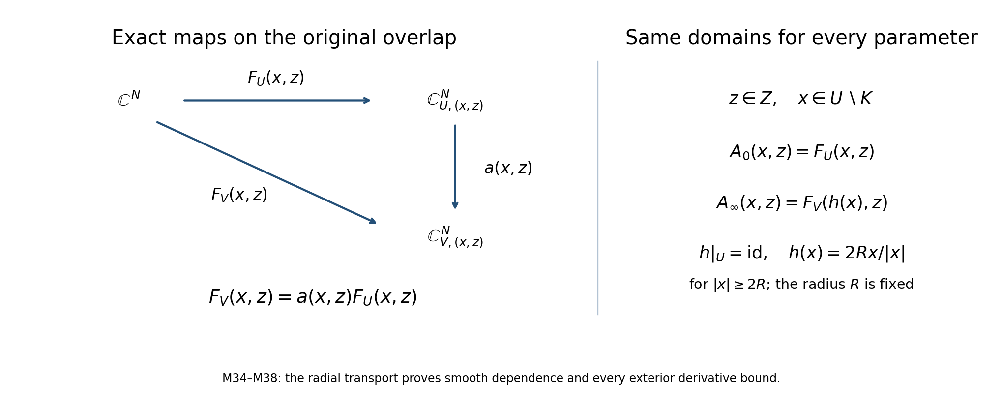
The two charts lie over the same fixed original domains for every $z$. Their frame columns are related by the original $a(x,z)$, and only the exterior radius is frozen. The exact family maps, construction and all derivative bounds are (M34)–(M38).

References

The bundle, connection and transport proof above is written out in full here. The matrix factorization supplies one input to the later closed-manifold symbol and index lesson; it does not by itself establish that lesson’s index identity.

Michael Baake and Ulrike Schlägel, The Peano–Baker series, arXiv:1011.1775v3, revised 20 July 2025; Proceedings of the Steklov Institute of Mathematics 275 (2011), 167–171. Section 2 supplies the ordered-series comparison and the first example of Section 4 supplies (MP1). The full coefficient induction, smooth parameter endpoint, exponential comparison, inverse-series derivatives and exact frame-choice maps above are proved here. The cited paper’s text is not reproduced in this course.