The Bott operator, suspension, and reduction of the index to Euclidean space
Written by Claude Opus 5.5 (Anthropic), September 2026. Self-checked by the writing AI. Public domain (CC0).
Edited and supplemented by Codex, September 2026. The additions and editorial corrections are also public domain (CC0).
This lesson moves the index of an elliptic operator on a compact manifold to an operator on a Euclidean space. The route has four steps.
- We build one operator of index one on , the Bott operator. It uses only the Euclidean structure of , so it commutes with the orthogonal group. Its index is computed from an energy identity for the harmonic oscillator (Sections 2–8).
- We combine an elliptic symbol on a compact manifold with the Bott symbol along the fibres of a Euclidean vector bundle over , and we prove that the index does not change. This is the suspension theorem (Sections 9–11).
- We embed in some . Its normal bundle is then diffeomorphic to a tubular neighbourhood of , and every vector bundle over a compact manifold becomes trivial after adding a suitable complement (Section 12).
- We apply the suspension theorem to the normal bundle, trivialize the bundles, and move the operator into the tubular neighbourhood. The result is a square system on that equals the identity outside a compact set and has the same index as the operator we started with (Section 13).
After this reduction, an index formula for systems on Euclidean space that are trivial at infinity gives an index formula on every compact manifold. The same strategy, carried out in K-theory, is the embedding proof of the Atiyah–Singer index theorem.
The lesson assumes the index theory of elliptic pseudodifferential operators on a compact manifold, including the index of a continuous symbol and its homotopy invariance, from the lesson Symbols, finite defects, and the index on a closed manifold. It also uses Fredholm theory in Banach spaces (Finite defects under perturbation), the Euclidean symbol calculus (From symbol estimates to operators on every Sobolev scale), symbols for a slowly varying metric (Localizing symbols when the measuring scale moves, Two measuring scales, one Weyl product and When a moving symbol scale controls an operator), and pseudodifferential operators on manifolds (Detecting regularity without choosing coordinates). The facts we use are stated in full in Section 1.
The proof inputs are the linked course lessons; Section 17 writes out the additional receiving arguments.
1. Conventions and background
Conventions
- . The Fourier transform is , and a symbol acts by left quantization, This is the convention of the lessons From symbol estimates to operators on every Sobolev scale and Symbols, finite defects, and the index on a closed manifold.
- Inner products are linear in the first argument: . Norms without a subscript are norms.
- . For we write .
- A metric on is a field of positive definite quadratic forms. For a metric and a positive function (a weight), the class consists of the smooth functions on such that, for every , for all . The best constants are the seminorms of .
- The classes and on have bounds uniform in : . “Classical” means polyhomogeneous: for large , has an asymptotic expansion in terms that are homogeneous in of degrees . Symbols may take values in linear maps between fixed finite-dimensional Hermitian spaces; products keep their order.
- Manifolds are Hausdorff and second countable. A compact manifold has no boundary. On a compact manifold, is the space of classical pseudodifferential operators of order from sections of to sections of . Usually and contain the factor , the bundle of half-densities, so that the pairing of sections needs no choice of measure. The geometric adjoint of is its adjoint for this pairing and the Hermitian metrics. The symbol index of a continuous symbol is recalled in Fact 1.13. By a homotopy of continuous symbols we mean a jointly continuous family that is invertible outside one compact set; by Fact 1.13(a) it preserves .
- Two metrics on recur: The first treats and alike; it is the natural metric for the harmonic oscillator. The second is a product metric.
Proofs used from earlier lessons
The following facts are proved in the preceding course lessons linked after each statement. Their hypotheses and conclusions are stated here so that each application can be checked at its full generality. Operators between Banach spaces are bounded and linear. An operator is Fredholm if its kernel and its cokernel are finite-dimensional; its range is then closed, and its index is .
Fact 1.1 (Compactness test). An operator between Banach spaces has finite-dimensional kernel and closed range if and only if every bounded sequence for which converges has a convergent subsequence. In that case, for every closed complement of there is with for all . See Finite defects under perturbation.
Fact 1.2 (Small perturbations). If is Fredholm, there is such that for every with the operator is Fredholm, , and . See Finite defects under perturbation.
Fact 1.3 (Products, sums and parametrices). If and are Fredholm, then is Fredholm and . A finite direct sum of Fredholm operators is Fredholm, and its index is the sum of the indices. A bounded bijection has index . If and there are such that and are compact, then is Fredholm. See Finite defects under perturbation.
Fact 1.4 (Strongly continuous families). Let be a compact space, and let and , , be strongly continuous: and are continuous for each and each . Suppose that the families and are collectively compact: the set of all with and has compact closure, and likewise for the other family. Then every is Fredholm, the function is upper semicontinuous, and is locally constant, hence constant when is connected. See Finite defects under perturbation.
Fact 1.5 ( boundedness). There is an integer , depending only on , with the following property. If is a smooth matrix-valued function on whose derivatives of order at most are all bounded by , then for , so extends to a bounded operator on . This is a form of the Calderón–Vaillancourt theorem. See From symbol estimates to operators on every Sobolev scale.
Fact 1.6 (Kernels of operators of low order). If with , the Schwartz kernel of is a continuous function, and for every . See From symbol estimates to operators on every Sobolev scale.
Fact 1.7 (Composition and asymptotic sums). If and , then with , and for every . If and , there is with for every , and with . See From symbol estimates to operators on every Sobolev scale.
Fact 1.8 (Elliptic parametrices). Let take values in square matrices and be uniformly elliptic: for all , all and . Choose with for large , and put and , which lie in . Asymptotic sums of the series and give with and in . Consequently, if for some and , then ; in particular is smooth. See From symbol estimates to operators on every Sobolev scale.
Fact 1.9 (Composition for a slowly varying metric). Let be the symplectic form on . For a metric , let be its dual metric, and its Planck function. Assume: - is slowly varying: there are such that implies ; - is symplectically temperate: , and for all ; - .
Let the weights be -continuous ( implies ) and temperate (). If and , then on , and . Each seminorm of is bounded by a constant times a product of finitely many seminorms of and of , and the constant depends only on , on the seminorm and on the constants in the hypotheses. See When a moving symbol scale controls an operator.
The complete split-metric receiving proof is Section 17.1, (P261.1)–(P261.7). It combines Quadratic Fourier multipliers at a moving scale, Theorems 7.1 and 8.1 and (G24)–(G26), Two measuring scales, one Weyl product, (W31)–(W34), and From Weyl symbols to operators and changes of coordinates, (A21), (A25), (A33)–(A43).
In Facts 1.10–1.16, is a compact manifold and are Hermitian vector bundles over it.
Fact 1.10 (Rellich compactness). For the inclusion is compact. We also use the local form: a set of distributions on that are supported in one fixed compact set and bounded in is relatively compact in . See Symbols, finite defects, and the index on a closed manifold.
Fact 1.11 (The elliptic alternative). Let be elliptic. Then is Fredholm for every . The kernel of and the kernel of its geometric adjoint consist of smooth sections and do not depend on , and . The kernel and cokernel have the same dimensions when acts on smooth sections. The index of a product of elliptic operators is the sum of their indices, and a formally self-adjoint elliptic operator has index . See Symbols, finite defects, and the index on a closed manifold.
Fact 1.12 (Building operators). If is a coordinate chart of over which and are trivial, then a classical operator of order on whose Schwartz kernel has compact support in defines, after extension by zero, an element of . For every smooth section of over that is homogeneous of degree , there is with principal symbol . See Detecting regularity without choosing coordinates.
Fact 1.13 (The index of a continuous symbol). Let be a continuous section of over that is invertible outside a compact set . Let be the length function of a Riemannian metric on the fibres of , and choose with . The radial restriction is a continuous invertible symbol of degree on . A smooth symbol that approximates it closely enough, uniformly on the unit cosphere bundle, is elliptic; the index of any of its quantizations is the symbol index , and it does not depend on the choices. It has these properties. - (a) Homotopy invariance. If , , is jointly continuous in and every is invertible outside one compact set, then does not depend on . - (b) Agreement with the index. If is elliptic, then , where is the principal symbol of , extended in any continuous way across a neighbourhood of the zero section. - (c) Smoothing. A continuous section of a vector bundle over the compact cosphere bundle can be approximated uniformly by smooth sections. - (d) Reduction to degree one. If every component of has positive dimension, then is homotopic, through continuous symbols invertible outside one compact set, to a symbol that is homogeneous of degree , smooth and invertible off the zero section. - (e) Zero-dimensional components. If is a finite set, then . In general the symbol index is the sum of its values on the components of .
See Symbols, finite defects, and the index on a closed manifold.
Fact 1.14 (Norm limits). Let , and let be a linear map on smooth sections that extends to bounded maps with for every real . Suppose that the principal symbols of the converge, uniformly on the unit cosphere bundle, to a continuous symbol , homogeneous of degree and invertible on . Then is Fredholm for every . The kernels of and of its geometric adjoint consist of smooth sections and do not depend on , the range of is the annihilator of , and . See Symbols, finite defects, and the index on a closed manifold.
Fact 1.15 (Partial operators). Let , with dual variables . Let be a classical symbol of order in , with symbol bounds uniform in and principal part , and let act in with as a parameter. Then maps to for every real . Moreover there are classical operators , , of order on with for every real , whose principal symbols differ from (extended by at ) by at most on the unit sphere . See Symbols, finite defects, and the index on a closed manifold.
Fact 1.16 (Products of symbols). Let and be compact manifolds. Let be a continuous symbol on from to , and one on from to , both invertible outside compact sets. On , the block symbol , from to , is invertible outside a compact set, and . This holds also when or is a finite set. See Symbols, finite defects, and the index on a closed manifold.
Fact 1.17 (Differential topology). The inverse function theorem. Smooth partitions of unity exist subordinate to every open cover, with the support of each function a closed set inside its member of the cover. Green’s formula holds for the nonnegative Laplace–Beltrami operator of a compact Riemannian manifold , applied to each component of a vector-valued function.
The complete inverse, subordinate-support partition and Green proofs are Section 17.2, (P261.8)–(P261.15). Their independent calculus, compactness, cutoff and inversion entries are Metric and topological foundations, Sections 5, 9, 12.4–12.8, 13.4–13.6 and 14.2.
Fact 1.18 (Hilbert spaces). Riesz representation: every bounded linear functional on a Hilbert space is for a unique . An integral operator whose kernel lies in is compact on , and its norm is at most the norm of the kernel.
The complete linear-first Hilbert representation and compact-kernel receiver are Section 17.3, (P261.16)–(P261.20). See also Lower-bounded spectral calculus, Section 2.3, (PR37)–(PR38), and Banach and Hilbert foundations, (LP3)–(LP4), (LP10)–(LP12), for product integration, completeness and compact smooth density.
Fact 1.19 (Integration and compactness). Dominated convergence. The Arzelà–Ascoli theorem: a set of continuous functions on a compact metric space that is uniformly bounded and equicontinuous is relatively compact in the uniform norm.
The complete dominated-convergence and Arzelà–Ascoli receivers are Section 17.4, (P261.21)–(P261.23). Their independent integration and metric compactness providers are Banach and Hilbert foundations, Section 15.1, (LP1)–(LP2), and Section 16.1, and Metric and topological foundations, Sections 7 and 14.1.
Fact 1.20 (Distributions with zero gradient). A distribution on a connected open subset of whose first partial derivatives all vanish is a constant function.
The complete compact primitive decomposition and connected-domain distribution proof are Section 17.5, (P261.24)–(P261.27). Their cutoff, coordinate integration and derivative entries are Metric and topological foundations, Sections 5 and 13.4–13.6, and Banach and Hilbert foundations, Sections 15.1 and 15.5.
2. The model on the line
We need an operator of index one on that uses only the Euclidean structure. In one dimension there is a simple candidate: , which is times the annihilation operator of the harmonic oscillator. First we fix the space on which it acts.
Definition 2.1. Let with derivatives in the sense of distributions. For a finite-dimensional Hermitian space we write for the -valued functions whose coefficients lie in .
Lemma 2.2. (1) is a Hilbert space, and is dense in it. (2) The inclusion is compact.
Proof. (1) If is Cauchy in , then , and converge in to some . Limits in are limits in distributions, so and . For density, fix with and for , and put . Fix with . For , dominated convergence gives and in . Also . So compactly supported elements are dense. If vanishes outside the ball of radius , let with a mollifier supported in . Then , and in . All supports lie in the ball of radius , so .
- Let be bounded in , say . For each , the functions are bounded in and vanish outside the ball of radius . By the local form of Rellich’s theorem (Fact 1.10), has an -convergent subsequence. The tails are small uniformly: . Take successive subsequences for and then the diagonal subsequence. For it, , so it is Cauchy in .
Proposition 2.3 (The model). Let , , , and . Then for is bounded and surjective, its kernel is spanned by , and is Fredholm of index .
Proof. Identity (2.2). For , , and . Both sides of (2.2) are continuous in the norm of , so Lemma 2.2(1) extends the identity to . In particular .
Kernel. If as a distribution, then . A distribution on with zero derivative is constant (Fact 1.20), so , and this function lies in .
Closed range and finite kernel. We use the compactness test (Fact 1.1). Let be bounded in with convergent. By Lemma 2.2(2) a subsequence converges in . Apply (2.2) to differences: . So the subsequence is Cauchy in . Hence has finite-dimensional kernel and closed range.
Dense range. Let be orthogonal to . Then for every . As a distribution this says , so and . This is in only if .
A closed dense range is everything, so is surjective. The index is .
The adjoint direction behaves in the opposite way: is injective on and its range has codimension one (Exercise 14.1). Proposition 2.3 is the case of Proposition 4.4 below: for the operator of Section 4 is exactly .
3. The exterior algebra and the odd–even symbol
To go from one dimension to , we need a matrix-valued symbol , linear over in , whose values are invertible for . The exterior algebra provides one.
Let be the exterior algebra of . We give the inner product , and the inner product with different degrees orthogonal. For put . These vectors form an orthonormal basis. Write and . For let and let be its adjoint. Put , , and .
Lemma 3.1. (1) Let . Then if and otherwise; if and otherwise.
- For all :
- , , , and Also : the operator multiplies a form of degree by .
Proof. (1) To write in increasing order, move past the elements of that are smaller than ; each move gives a factor . If with , then , and all other inner products vanish; this gives .
The first relation is ; the second is its adjoint. For the third, take first. If then (the two signs are equal) and ; if the roles swap. Now let . Both and vanish unless and . Then both are multiples of , : If , then and . If , then and . In both cases the two terms cancel.
The first two formulas follow from linearity of and conjugate-linearity of the adjoint. . By (3.1), . Finally for and otherwise.
Proposition 3.2. Let .
- (Koszul complex.) The sequence , with every map equal to , is exact.
- (Odd–even symbol.) Let and . The adjoint of is , and So is invertible, , and is unitary.
- If , then . If , then and .
- For , on . So is real-linear in .
- For let act by . Then is unitary, preserves and , and
Proof. (1) , so each range lies in the next kernel. If , then (3.2) gives , so is in the range. (The map is a contracting homotopy.)
is self-adjoint and changes the degree by , so it maps to and back. Since , the adjoint of is . By Lemma 3.1(3), . Restricting to and to gives (3.3).
If , is unitary from onto , so the dimensions agree; they add up to . This matches the count . If , .
This is Lemma 3.1(3) with .
is real and orthogonal, so it preserves on . The determinant formula then shows that preserves inner products, and it is invertible with inverse . It preserves degrees. From we get . Taking adjoints and using unitarity gives . Add the two identities and restrict to .
Remark 3.3. The invertibility of is the finite-dimensional case of a general fact about complexes: for an exact complex, the odd–even operator , from the even to the odd part, has zero kernel, and its index is the Euler characteristic, which is zero. See Traces that survive passage to cohomology. The identity (3.3) gives more: an explicit inverse, with norm .
Example 3.4 (Two small cases). For , , , and ; so is multiplication by . For , in the bases of and of , Indeed , and by Lemma 3.1(1).
4. The Bott oscillator
We now replace by the operators . The result is an operator of index one on for every .
A form on is a function with values in ; operators on functions act on each coefficient . Put Thus and come from and in Lemma 3.1(3) when replaces and replaces . By Proposition 3.2(4), the symbol of is . Each term contains either or alone, so every quantization gives the same operator. We write and , regarded as a form of degree . Here is the space (2.1).
Lemma 4.1 (Algebra). On smooth forms, and on distributions: 1. , , . 2. , where is the exterior derivative. Also and . 3. With the degree operator of Lemma 3.1, 4. on each coefficient.
Proof. (1) Using : , while , and similarly for . (2) . In the factor is symmetric in and is antisymmetric by (3.1), so the sum vanishes; the same argument works for . (3) The scalar operators commute with the constant matrices . Writing , by (3.1). (4) .
Lemma 4.2 (Energy identity). For with degree components , Consequently For an even form and an odd form in ,
Proof. First let . Integration by parts gives , and . So is the formal adjoint of and is formally symmetric. Then (4.1) gives , which is (4.2). For (4.3), on each coefficient , and . Both identities have sides that are continuous on , so Lemma 2.2(1) extends them. By (4.2)–(4.3), , which gives the first inequality in (4.4). For the second, by (4.3) and . Finally (4.5) is (4.2) with replaced by or .
Lemma 4.3 (Regularity). If and in the sense of distributions, then .
Proof. Let be a mollifier supported in with , let , let with as in Lemma 2.2, and put . Then in . We bound , using . - Convolution commutes with , and has norm at most , because . - The matrices have norm : by (3.1), and , and the first is self-adjoint, the second skew-adjoint. - , and the last term has norm at most .
Together, By (4.4), for all . Now fix a coefficient and a scalar test function . Then , so . The distribution , which acts by , is therefore bounded in the norm on a dense subspace. By the Riesz representation theorem (Fact 1.18) it is an function. The same argument with shows . So .
Proposition 4.4 (The Bott oscillator). Let . 1. is bounded and surjective, its kernel is spanned by , and is Fredholm of index . 2. If and in the sense of distributions, then . If and in the sense of distributions, then . 3. , with domain , is a self-adjoint operator on . Its kernel is , and for every odd .
Proof. (1) is bounded by (4.4). Kernel. If and , then (4.5) gives for and for all . Then . A distribution on the connected set with zero gradient is constant (Fact 1.20), so . Conversely , so , and .
Closed range. Let be bounded in with convergent. By Lemma 2.2(2) a subsequence converges in , and (4.4) applied to differences shows that it is Cauchy in . By the compactness test (Fact 1.1), has finite-dimensional kernel and closed range.
Dense range. Let be orthogonal to . Testing with and using the formal symmetry of , we get as a distribution. By Lemma 4.3, , and then (4.5) gives . So .
The range is closed and dense, so is surjective, and .
Apply Lemma 4.3 (with or ), then part (1) or (4.5).
is symmetric on : the identity holds on and extends by (4.4) and density. If is in the domain of the adjoint, then is -bounded on test forms, so the distribution lies in . By Lemma 4.3, . So the adjoint has the same domain and is self-adjoint. The kernel and the lower bound follow from (4.2) and (4.5) as in (1).
Remark 4.5 (The weighted identity behind (4.2)). By Lemma 4.1(2), is the exterior derivative conjugated by . If , then , and corresponds to the adjoint of in . So (4.2) is an identity for the de Rham complex with the weight , . The commutator is the Hessian of , and the term is that Hessian acting on forms of degree . The same mechanism, in degree one and for in place of , underlies Hörmander’s paper, L² estimates and existence theorems for the ∂̄ operator, Acta Mathematica 113, pages 89–152, on estimates for : for a strictly plurisubharmonic weight , the equation , with a -closed form, can be solved in . The key identity there is for forms of type , and it comes from the commutator of the weighted adjoint with , which is : the complex Hessian of the weight takes the place of . We do not use that theorem.
5. Lowering the order to zero
The operator has order one in both and . The truncation in Section 6 needs an operator of order zero. We compose with an operator that maps onto . First we record how quantization interacts with the coordinate functions.
Lemma 5.1 (Exact composition rules). Let be a smooth symbol on whose derivatives grow at most polynomially. On Schwartz functions,
Proof. The first rule holds because , and the third is immediate from the definition of . The second follows from and an integration by parts in . The fourth follows by differentiating under the integral sign, since .
Remark 5.2 (A parametrix for the Bott oscillator). Proposition 4.4 can also be proved with a parametrix. Take equal to outside a compact set. By (3.3) this inverse is , which is homogeneous of degree ; so with from (1.1). The operators and have symbols in , whose derivatives are all bounded, so they are bounded on by Fact 1.5. Thus . Since the symbol of is affine in , (5.1) gives the compositions exactly: Both errors lie in . Then maps into , so it is compact on by Lemma 2.2(2), and the range of is closed of finite codimension. In the same way maps into . So if and , then lies in ; Lemma 4.3 gives this without a parametrix. Iterating, , one can show that a tempered solution of is a Schwartz function. That needs the mapping properties of on tempered distributions, which we do not develop.
Now we lower the order. For and put So is the metric of (1.1). We use the symplectic form , the dual metric and the Planck function of Fact 1.9, as in the lessons Two measuring scales, one Weyl product and When a moving symbol scale controls an operator.
Lemma 5.3 (Uniform structure). Let . 1. and . 2. , so with Planck function . Also . 3. is slowly varying and symplectically temperate, in the sense of Fact 1.9, with constants independent of . 4. For each real , the weight is -continuous and temperate in the sense of Fact 1.9, with constants independent of , and with seminorms independent of .
Proof. (1) is immediate. (2) Since , we have . The map (the covector ) is an isometry for the Euclidean norm, so the supremum is . Then .
- First let .
Slow variation. The function is -Lipschitz. If , then . Hence , and the forms and agree within the factor .
Temperance. Since is -Lipschitz and , and . Moreover So . Since and , the ratios and have the same bound.
General . By (1), the slow-variation condition for at is the one for at . For temperance, . So the temperance inequality for at implies the one for , with the same constants.
- is a classical symbol of order on : . So , that is, . By (1), , and the same bound holds with and the same . Temperance of the weight follows from the bound in (3), and its -continuity from slow variation.
So and the weights satisfy the hypotheses of Fact 1.9 with constants independent of , and the constants in Fact 1.9 depend only on these, on the dimension and on the orders. Hence, for and , where are powers of , we have on , and , with seminorm bounds independent of .
Lemma 5.4. There is such that for the operator is an isomorphism of onto . Moreover in as , for every .
Proof. (a) maps into . By (5.1), and . For fixed these symbols are bounded with all derivatives bounded (for example ), so Fact 1.5 bounds the operators on .
maps into , uniformly in . On , (5.1) gives the exact identity Indeed the second sum has symbol , the third has symbol , and . Now , , and a derivative in a unit direction costs the factor . So all derivatives of and are bounded by , and all derivatives of by , with independent of . By Fact 1.5, first on and then on by density.
Compositions. By Lemma 5.3 and Fact 1.9, and , where are bounded in uniformly in . So and on .
bounds. For bounded in , . By Fact 1.5, .
bound. By (5.1), and . For these symbols are bounded in , so the commutators have norm at most . Hence , first on , then on .
Invertibility. Choose so that in (d) and (e). The identities in (c) extend by continuity and density: the first to , the second to , using (a) and (b). Then is invertible on and on , by the Neumann series. If , then , so . If , then satisfies . So is bijective, with the bounded inverse
Convergence. For , The first term is at most , by (b) and (e). For the second, (b) gives a bound uniform in , so it is enough to take . By (5.2), in . Finally in . For each , by dominated convergence in , since and . These functions have the common bound , obtained from , an integration by parts, and the uniform bounds . Dominated convergence in gives convergence in .
Corollary 5.5 (The order-zero oscillator). Fix with and . This is possible because by Lemma 5.4, so every small qualifies. (The bound is used in Theorem 7.4(v) and Proposition 8.2.) Let act on each coefficient, and put . 1. is bounded, surjective and Fredholm of index . Its kernel is spanned by , a form of degree . So is injective on the forms with . 2. , where 3. . There is such that is invertible for , with , and the derivatives of satisfy the bounds of on . 4. for .
Proof. (1) is an isomorphism of onto (Lemma 5.4), and is surjective of index (Proposition 4.4). The composite is surjective, and its index is by Fact 1.3. Its kernel is . If and , then and , so .
The symbol is affine in , so (5.1) gives exactly. With : by Proposition 3.2(4), and . So the correction is , since and for real .
. For fixed , , so (the metrics and are comparable, with constants depending on ). Hence and the correction lies in . By (3.3), has norm when . The correction has norm there, because . So for , with , and . Differentiating gives ; by induction every derivative of order is a sum of products of and derivatives of of total order , hence .
Use (3.4), the invariance , and .
The lower-order part of (5.3) matters later: after the truncation of Section 6 it is homogeneous of degree zero in , so it survives in the principal symbol of the Bott operator (Theorem 7.4(v)).
6. A truncation that is uniform in the product metric
The Bott operator of Section 7 must be classical of order , and it must act as a multiplication for large . We obtain it by deforming the symbol . This section provides the deformation: it makes a symbol homogeneous of degree for large and independent of for large , with bounds that are uniform in the product metric .
Cutoffs. Fix radial functions and , both decreasing in , with Such exists. Take , , on , on , with (so exceeds somewhere in ), and put with . Then is increasing, on and for . Two consequences of (6.1) are used below: on ; and for every . (For , . For , . For , .)
Lemma 6.1 (Uniform truncation). Let and let , with values in a fixed space of matrices. Equivalently, Every has this property. For put 1. The family , , is bounded in : with constants independent of . 2. . If , then . If , then , which is homogeneous of degree in . 3. is jointly continuous in .
Since , we have . The first inclusion is strict: lies in but not in , because is of size , not , when . The proof below needs only (6.2). Example 6.2 shows that is not enough.
Proof. Parts 2 and 3 follow from (6.1) and the continuity of . For part 1 we split into regions.
Reduction to . On the closed set , is homogeneous of degree ( for ), so is homogeneous of degree there. Given with , put , so . If the bound holds at , then and because . So it suffices to prove the bound where . The three regions below cover all .
Region . Here and with . Since , . For , , and is smooth, and it is homogeneous of degree where . Hence, for , The second step uses and . For , and the bound is trivial. By the chain rule, is a finite sum of terms By (6.2) and up to a constant, each term is at most .
Region . Here . All -derivatives vanish and by (6.2). By continuity this also holds where .
Region . Here and . By (6.2), since , Also with . Since has compact support and is homogeneous of degree for , . Hence The chain rule writes as a sum of terms with , and . Write each factor as . The from cancels the , and each term is at most .
Example 6.2 (The product class is not enough). Let with on and on , and . This symbol lies in , but not in , since does not decay in where . Let (we write for the value at ); on . For and , Lemma 6.1(2) gives . Along a ray, as runs from to , this falls from to . The fall happens where , that is, on with . Since is continuous and positive on , as . By the mean value theorem some on this segment has , while . So : the family is not bounded in . So the derivatives of in its second slot must also gain the factor , as (6.2) requires through .
7. The Bott operator
The Bott operator is obtained from the order-zero oscillator of Corollary 5.5 in three moves: truncate its symbol by Lemma 6.1, cut off the far part of its kernel, and normalize it at infinity. We first collect three tools.
Lemma 7.1 (The product metric). The metric of (1.1) has dual metric and Planck function . It is slowly varying and symplectically temperate, and . The weights and are -continuous and temperate in the sense of Fact 1.9. Consequently, for bounded in , on , and is bounded in , with bounds depending only on finitely many seminorms of and .
Proof. By definition, is the supremum of over . Substitute and . Then and , so by Cauchy–Schwarz the supremum is . The ratio of the corresponding terms of and is for both, so . Also . If , then and , so and lie in ; this is slow variation. For temperance, and ; the same holds for and for the inverse ratios. This bounds , and by . The last statement is Fact 1.9 with .
Lemma 7.2 (Families). Let be a compact metric space. 1. (Strong continuity.) Let symbols , , have all derivatives bounded uniformly in , and let be continuous for each . Then and is continuous in for every . 2. (Collective compactness.) If , , is bounded in , then the family is collectively compact on : the set has compact closure.
Proof. (1) The uniform bound is Fact 1.5. Let and . For each , by dominated convergence in . Integrating by parts with , and using the uniform bounds on , gives uniformly in . Dominated convergence in gives convergence in . For general , approximate by Schwartz functions and use the uniform bound.
- Fix with , on , for , and put .
Far part. On the support of every derivative of is bounded by , and every derivative of of positive order is at most . So all derivatives of up to any fixed order are at most , and by Fact 1.5, for all .
Near part. Let , supported in , and . The function vanishes for . By Cauchy–Schwarz on the ball and Plancherel, and , uniformly in and : a derivative falls either on , giving a factor of size at most , or on . By the Arzelà–Ascoli theorem (Fact 1.19) these functions form a relatively compact set in , hence in .
Given , choose with and a finite -net for the images of the near parts. It is an -net for the whole family of images. So that family is totally bounded.
Lemma 7.3 (Orthogonal symmetry). For and a form put . (For forms of degree this is the pull-back of by .) 1. is unitary on , preserves degrees, and preserves , and . 2. Let be a symbol with bounded derivatives, or a polynomial in , with values in or between parts of , such that Then on , and on when is bounded there. Scalar symbols that depend only on and satisfy (7.1). 3. A continuous even form with for all is a scalar function of times . 4. Let be a one-dimensional subspace of with for all . If some with for all satisfies for , then for all and all .
Proof. (1) Change variables and use unitarity of (Proposition 3.2(5)).
The Fourier transform of is . Substituting , so that , They agree by (7.1) with .
At : let be the reflection in . Then if and otherwise, so invariance kills every component with . At : choose an orthonormal basis and expand in the corresponding basis of . The reflections in , , fix , so invariance kills every with . What remains is spanned by and , and is even, so . The scalar then satisfies , so it depends only on .
Since is one-dimensional and invariant, for a scalar . By unitarity, , so .
Part 4 needs no average over the orthogonal group, and no continuity in .
Theorem 7.4 (The Bott operator). Let . There are numbers and a symbol with these properties. - (i) for . - (ii) The Schwartz kernel of minus has compact support. - (iii) is surjective. Its kernel is spanned by one function of degree that depends only on . - (iv) for every . - (v) For the principal symbol is , where, with , Every singular value of is at least , and . So is invertible for , and every point of the segment from to is invertible.
Construction note: For the literal construction here the principal symbol is , and at every with , as Step 8 proves.
Proof. Step 1 (the inverse symbol). Fix as in Corollary 5.5, so with . Let be a smooth function of , equal to for and for , and put . Let and . Outside we have , so there. Both and satisfy (7.1).
Step 2 (truncation). For , let and be the truncations (6.3) of and of . By Lemma 6.1 they are bounded in and continuous in . They satisfy (7.1), because . We claim outside . Indeed , which is unless . In that case , so and . Then , and since for , we get . So , , and .
Step 3 (index one). By Lemma 7.1, and , where is bounded in : the first bracket by Lemma 7.1, the second because it is supported in the compact set , where is bounded below. The same holds for . The operator identities hold on , hence on . By Lemma 7.2, and are strongly continuous in , and the errors form collectively compact families. Fact 1.4 now gives three conclusions. Every is Fredholm. Its index is constant, hence equal to . And since the kernel dimension is upper semicontinuous, there is with for . For those the kernel has dimension exactly and the cokernel is .
Step 4 (the kernel is invariant). Let span , . We claim for all small . If not, take with . Since , collective compactness gives a subsequence converging in to some with . Then by strong continuity and the uniform bound. So and , which Corollary 5.5(1) excludes. Fix such a . The kernel is invariant under every , by Lemma 7.3(2), and is invariant, so Lemma 7.3(4) shows that is invariant. For , Lemma 6.1(2) gives with : if , then . So is invertible there, with inverse bounded. Thus is uniformly elliptic in , Fact 1.8 gives , and is smooth. By Lemma 7.3(3) it is a scalar function of .
Step 5 (the kernel near infinity). Let be the Schwartz kernel of . - (a) For , for all , so ; that is, there. - (b) Off the diagonal is smooth and for . Indeed is, up to a power of , the kernel of , whose symbol has order . By Fact 1.6, such a kernel is continuous and rapidly decreasing in when ; derivatives in and are handled by taking larger.
Step 6 (cutting the far part of the kernel). Let . Put The kernel of is . It vanishes for by Step 5(a). If and , then , so and only contributes. By Step 5(b), is smooth, vanishes unless and , and satisfies . So as . By Fact 1.2, for small , is Fredholm of index with kernel of dimension at most ; so it is surjective with a one-dimensional kernel. satisfies (iv) because is radial and satisfies (7.1).
Let span , , and put . Then is orthogonal to , and . By the lower bound of Fact 1.1 for on the orthogonal complement of its kernel, . So . Fix with . Lemma 7.3(4), with , shows that is invariant.
For , Step 5(a) gives . Here is invertible, because . So vanishes for . The principal part of the symbol of is (for both terms equal ), and the other terms of the composition have order by the composition formula of Fact 1.7. So is uniformly elliptic, is smooth by Fact 1.8, and by Lemma 7.3(3) is a smooth compactly supported scalar function of .
The kernel of is . For it equals , so there. For the second term vanishes and the first is supported in . So the kernel of minus is supported in .
Step 7 (normalization at infinity). Put a smooth positive radial function (the last factor is finite because ). For , , , and by (5.3) with . Choose with . For put For , and is unitary, so is invertible. Define for and for . On the overlap we have and , so the two formulas agree there, and is smooth. is invertible at every point, it satisfies (7.1), and , and all derivatives of are bounded: for , . Now set We check (i)–(iv). - (i) For , and , so . - (ii) The kernel of minus is times the corresponding kernel of . - (iii) , spanned by , and is surjective because is a bounded bijection of . - (iv) holds because and are equivariant.
is classical: is exactly homogeneous of degree for ; the composition has the expansion of Fact 1.7, whose terms are homogeneous of degree for large ; and multiplication by preserves this.
Step 8 (the principal symbol). For , and . By Lemma 6.1(2), with , and , so . With (5.3) this gives , since there. For , ; here , so and . So (7.2) holds everywhere.
Next, with ; is unitary by (3.3), and . So all singular values of are at least . Since and , . Then with , for . Finally, for and , , and , so .
Remark 7.5. The factor of Step 7 cancels in the first term of (5.3) but not in the second term . In the metric that term has lower order (it lies in ), but after the truncation it is homogeneous of degree in , so it stays in the classical principal symbol. This does no harm: every later use needs only the invertibility of for and its homotopy class, and part (v) gives both. The number is small for two reasons: must exceed and , so that is a multiple of wherever is not a multiplication, and , so that is invertible.
8. The Bott operator on the sphere
The suspension theorem needs an elliptic operator of index one on a compact manifold. We move the Bott operator to the sphere , the one-point compactification of .
Let , with the identity chart on and the chart (with ) on . The group acts on by , fixing and ; this commutes with the inversion, so the action is smooth. The metric is invariant under and under the inversion, so it is a smooth metric on (the round metric of radius ). The length of a covector at is .
Let . Let be the bundle glued from and by identifying with for and . The transition is smooth and unitary by (3.3), so is a smooth Hermitian bundle. We call the two descriptions the first and second trivializations of . acts on and on through in each description; by (3.4) the two actions agree on the overlap.
Proposition 8.1 (The Bott operator on the sphere). Let be as in Theorem 7.4, and choose such that the compactly supported kernel in (ii) vanishes unless . There is exactly one operator such that - (a) on , in the first trivialization, for every ; - (b) on , in the second trivialization, .
Moreover: - (c) is elliptic. Its principal symbol is over and the identity (second trivialization) near . - (d) The kernel of , on smooth sections or on any Sobolev space, is spanned by (extended by near ). maps onto , and . - (e) commutes with the action of .
Proof. Write , where is multiplication by and ; by (ii), the kernel of vanishes unless . So is a classical operator of order with compactly supported kernel in the chart , and by Fact 1.12 it defines an element of that vanishes near . For , , which is the identity in the second trivialization. So extends to a smooth bundle map on , equal to the identity near . Put . For , is smooth and bounded, hence tempered, and ; this is (a). For , , which gives (b). Uniqueness holds because (a) and (b) prescribe on an open cover.
The principal symbol of is , and that of is . Ellipticity is Theorem 7.4(v).
If for a distributional section , then by (b) on . So is a compactly supported distribution on , hence in some , with . is uniformly elliptic in , so Fact 1.8 gives , and by (iii). Conversely lies in the kernel. For surjectivity let . Choose a smooth radial on , equal to for and at , and for . Let be the section of that equals in the second trivialization. It vanishes for , so and . Next, . By (iii) there is with . For , , which vanishes for , and is invertible there. So has compact support, it is smooth by ellipticity, and . Hence . The index on smooth sections is , and by Fact 1.11 it equals the index on every Sobolev space.
follows from (iv) and the equivariance of and of the transition of .
Proposition 8.2 (The symbol class). For all large , the maps and , from the sphere to the invertible maps , are homotopic through continuous maps into the invertible maps.
So away from a compact set the symbol of is homotopic to . The name Bott operator comes from K-theory: on , the class of the symbol is the generator that appears in the Bott periodicity theorem. We do not use that theorem.
Proof. Take .
From to . Where both equal (Theorem 7.4(i), (v)). Where , is large. is classical of order with bounds uniform in , so there, while by (v). For large the segment from to consists of invertible maps.
From to . Use the segment, which is invertible by (v).
From to . Write with and . For use The scalar factor is positive. On , the argument of vanishes only if ; then and , so the imaginary part is not . All maps are continuous on : at points with we have , so nearby and there.
Example 8.3 (Dimension one). Let . Then , , , and is the model of Section 2. On , is multiplication by (into ), so (5.3) reads , and by (7.2), with , The correction rescales the real part by a factor in and never changes its sign. So it cannot change a winding number, which is the content of Theorem 7.4(v) in this dimension. On a large circle in the -plane the symbol winds once around , counterclockwise for the orientation . By Proposition 8.2, so does . This agrees with . It also agrees with the index formula for systems on Euclidean space mentioned in “Where this leads”: in dimension one it gives the index as for large , and here it serves only as a check.
9. The suspension theorem
We now combine an elliptic symbol on a compact manifold with the Bott symbol along the fibres of a Euclidean vector bundle over .
Setting. - (S1) is a compact smooth manifold, are smooth Hermitian vector bundles over , and is invertible outside a compact set . - (S2) is a smooth real vector bundle of rank with a Euclidean structure. Near each point of there is an orthonormal frame; a frame over an open set gives , and two frames differ by a smooth map . - (S3) is the fibrewise one-point compactification: , glued by . Since commutes with the inversion , this is a smooth structure, and in it extends to a diffeomorphism of onto ( is the zero section). is compact of dimension , and is a submersion. - (S4) . is glued from over and over , identifying with . In a frame, and , glued by ; this is well defined by the equivariance in Section 8. and . - (S5) For with , let , and let be the restriction of to the tangent space of the fibre at , which is ; we identify with a vector by the Euclidean structure. are real continuous functions of with , , and , for . (Real values are used in Theorem 9.2(1): if with real at some , then at , and the diagonal entries of (9.2) are not invertible there.) Finally satisfies
Such exist. Take smooth real functions with on and , and let be the restriction of to the horizontal space of frame (the tangent space of , which maps isomorphically onto ). Then is continuous and satisfies (9.1), because restricts to on every horizontal space.
Define from to . Where , the diagonal entries are and , which are the identity in the second trivialization of ; this defines at the section at infinity.
Lemma 9.1 (Block lemma). Let and be linear maps of finite-dimensional Hermitian spaces, and let be the block matrix of (9.2) with in place of and in place of . Then and are block diagonal with blocks , and , . If or is invertible, all four blocks are positive definite and is invertible.
Proof. Multiply out. The off-diagonal blocks cancel, because operators acting on different tensor factors commute; for instance the lower left block of is . If is invertible, then and are positive definite; the other term of each block is positive semidefinite, so every block is positive definite. The same holds if is invertible. Then and are invertible, so is injective and surjective. This is the pointwise algebra behind Fact 1.16.
Theorem 9.2 (The suspension theorem). Assume (S1)–(S5). 1. is continuous on and invertible outside a compact set. 2. does not depend on the choice of satisfying (9.1), nor on as in (S5), and it depends on only through its homotopy class. 3.
Proof of (1) and (2). (1) Continuity is clear away from the section at infinity; near it the diagonal entries are the identity in the second trivialization and is continuous. If or , then is invertible: , and forces and then . At infinity the diagonal is the identity. The remaining points have and . Then vanishes on the vertical space, which is the kernel of the surjection , so , and . By Lemma 9.1, is invertible outside , which is compact.
- If both satisfy (9.1), so does , and the corresponding are invertible outside the same compact set. By homotopy invariance (Fact 1.13(a)) they have the same symbol index. Convex combinations of admissible pairs are admissible (with the larger ), and the same argument applies. If is a homotopy of symbols invertible outside one compact set, then is continuous in and satisfies (9.1), so is unchanged.
Part (3) is proved in Section 10.
Example 9.3 (The condition is necessary). Let be a point, and . Then is a point, so is invertible outside a compact set, and . Here , and (9.1) only fixes on the zero section, so is allowed. With , is invertible except at . If instead , then at the diagonal entries vanish for every , so on an unbounded set and is not defined.
10. Proof of the suspension theorem
We prove (9.3). We realize a symbol homotopic to by an operator whose kernel and cokernel we can compute exactly. combines an operator along the fibres, built from the Bott operator, with a lift of an operator on . Neither part is a pseudodifferential operator on , so is reached as a norm limit of genuine ones, as in the proof of the product formula (Fact 1.16).
Step 0 (the full comparison with the original symbol). Keep the original symbol and the original block from (S1)–(S5). Section 16 gives the complete families linking them to the degree-two symbol used in the operator construction, and proves the exact receiving equalities (BQ6). In Steps 1–7 below the shorter letter denotes that specified degree-two symbol; the original remains explicit in (BQ1)–(BQ6). First let every component of have positive dimension; zero-dimensional components are treated in Corollary 10.1. By Fact 1.13(d), is homotopic to a symbol that is homogeneous of degree , smooth and invertible off the zero section. Multiply it by , where is the length for a Riemannian metric on . This is a homotopy through symbols invertible off the zero section, and it ends at a symbol homogeneous of degree . So from now on is homogeneous of degree , smooth and invertible on . We take , and in we take the cutoff , with from Theorem 7.4; both choices are allowed by Theorem 9.2(2).
Step 1 (an operator of order two on the fibre). Let be the Laplace–Beltrami operator of on , acting on each component of sections of the trivial bundle , and let . It is an elliptic differential operator of order with principal symbol . With the Riemannian volume of , Green’s formula (Fact 1.17) gives for smooth . So is formally self-adjoint and injective on smooth sections. By Fact 1.11 a formally self-adjoint elliptic operator has index ; hence is a bijection of smooth sections and an isomorphism for every . commutes with the action of , which acts by isometries and by the constant matrices . Put is elliptic of order with principal symbol . It is surjective, because is bijective and is surjective (Proposition 8.1(d)). Its kernel is spanned by , and it commutes with . The section is smooth and invariant, hence a scalar function of by Lemma 7.3(3). Since is surjective, its formal adjoint (for and the Hermitian metrics) is injective on smooth sections.
We use an operator of order two because it is easy to make invariant and invertible. A first-order operator with principal symbol that commutes with would need an invariant square root of an elliptic operator. The only cost of order two is that is taken homogeneous of degree in Step 0.
Step 2 (the fibre operator on ). Use the fibre volume to identify fibre half-densities with fibre functions; then . Over , a section of is a function of with values in . Let act by in , with as a parameter. A change of frame acts by , which commutes with ; so is well defined on . The same holds with in place of , and for , which acts by .
Step 3 (lifting ). Let each be a coordinate chart over which are trivial and has an orthonormal frame, with as in (S5). Let have principal symbol (Fact 1.12). In frame , let act by in , with as a parameter. Put , from sections of to sections of , and define on in the same way. Put ; its principal symbol is . - (a) If is a smooth function on that depends only on (so it is the same in every frame) and , then - (b) On smooth sections, - (c) In frame , acting in , with the geometric adjoint on ; similarly for .
Proof of (a)–(c). (a) In frame , acts in only, and depends only on . (b) In frame , acts in and in . Operators acting in different factors of commute on smooth sections: they commute on finite sums of separated sections, which are dense in the smooth topology, and both are continuous there. (This is the density argument used for products in Symbols, finite defects, and the index on a closed manifold.) Sum over . (c) In frame the pairing is the product of the pairing on and the pairing on , with the Hermitian metric of , which does not depend on the frame. Fubini’s theorem gives the adjoint.
Step 4 (the operator and its approximations). Let from sections of to sections of . Let It is continuous, homogeneous of degree in , and invertible on : if , is invertible by Proposition 8.1(c); if and , then with and is invertible; now use Lemma 9.1.
Claim. There are with for every real , whose principal symbols converge to uniformly on the unit cosphere bundle.
Construction. We follow the proof of the product formula (Fact 1.16), with the product replaced by the local products . Choose real functions on with , such that each lies in or in (so is trivial over it), and each union misses some point (small supports do this, since ). In frame , Editorial completion of the bundle frame in these charts. The target bundle is trivial on each punctured sphere , with a smooth frame that can be constructed as follows. If , use its original second trivialization; if , use its original first trivialization. Otherwise identify the punctured sphere with by the chosen stereographic coordinate , and let be the coordinate of the original point . Choose a bounded open ball around , with closure in the original first-trivialization chart, and set , . The first frame is defined on , and the second on all of . Let be their actual smooth invertible coordinate transition on , so a target vector has second coordinate . The matrix-extension theorem in Changing an interior frame to extend an invertible matrix, (M1)–(M3), supplies smooth invertible matrices on and on , with on the overlap. Their columns therefore define the same frame in both original bundle charts. This proves a global smooth frame on the punctured sphere, with a smooth inverse, without assuming a separate bundle-triviality theorem. The domain bundle already has its original global frame. These frames depend only on the sphere variable; in a fixed base frame they preserve the partial-operator form. The compact kernel cutoffs in the next paragraph keep all needed matrix and inverse derivatives bounded. No global bound near the omitted point is used.
- Each term of the first sum is a partial operator in the product chart , where by stereographic projection. It acts in the sphere variables, with the base variables as parameters. Its partial symbol is , where is the left symbol of in that chart: classical of order in , compactly supported in , with uniform bounds.
- Each term of the second sum is a partial operator acting in , with partial symbol , where is the local symbol of .
- The half-density identifications multiply these operators by fixed smooth positive functions of , which keeps the partial form.
Apply Fact 1.15 with to each term. Then multiply the approximants on both sides by fixed cutoffs that equal one near the supports of the exact terms, so that the exact terms are unchanged and the approximants have compact kernel support in their product chart; by Fact 1.12 they define elements of . The adjoint entries are treated the same way, using and . There are finitely many terms, so the operator estimate of Fact 1.15 gives the norm bound. By the symbol estimate of Fact 1.15, the leading symbols converge uniformly on the total cosphere bundle to the partial leading symbols, extended constantly in the other frequency. For the fibre terms the limit is , because the fibre frequency in every product chart is the restriction of to the fibre. For the base terms it is , because in the chart of frame the base frequency of is .
Step 5 (Fredholm property and index). Fact 1.14 applies to , with from (10.4) and limiting symbol from (10.5). So is Fredholm for every , the kernels of and of its geometric adjoint consist of smooth sections and do not depend on , and
Step 6 (kernel and cokernel). Here . By (10.3), For example the lower left entry of is , and the lower left entry of is ; the upper right entries are their adjoints. For smooth , , so , and likewise for . Each diagonal block is a sum of two nonnegative terms, so is injective on smooth sections, because is injective on each fibre. So the second summand of and the first of vanish.
A smooth with restricts on each fibre to an element of . So with , which is smooth. By (10.2), . Hence is an isomorphism of onto .
Next let with . We need to know when , that is, when for all smooth . preserves the fibre degree and has degree , so it suffices to take of degree . For a section of degree put . Then , and : in frame , acts in and is continuous on smooth sections, so it commutes with the integral in . As runs over sections of degree , runs over all of (take ). So if and only if for all , that is, . Hence . By Fact 1.14, ; by Fact 1.11, ; and by Fact 1.13(b), since has principal symbol . So
Step 7 (from to ). It remains to show . We deform the diagonal entries and keep . By Lemma 9.1 each intermediate symbol is invertible where , and where , it is invertible because of . So each family below is invertible off the zero section, which is compact, and only continuity has to be checked.
From to along : invertible for by Theorem 7.4(v), continuous, and at .
From to along At , real-linearity of gives ; at , . For , : the argument of vanishes only if , and then its imaginary part is because ; the scalar factor is positive. is continuous at because . Near the section at infinity, and , so , which is times the identity in the second trivialization; and is continuous on .
The lower right entries are deformed by the adjoint families.
So , with formed from , and , and by Theorem 9.2(2) this is for every admissible choice. With (10.6) and (10.7), .
Corollary 10.1 (The Bott symbol has index one; zero-dimensional bases). 1. Let on , a continuous symbol from to that is the identity near in the second trivialization and invertible except at . Then . 2. Theorem 9.2(3) also holds when has zero-dimensional components.
Proof. (1) For of (10.1), by Fact 1.3, so the principal symbol has symbol index by Fact 1.13(b). Steps 7(a)–(b), without the block with , deform it to through symbols that are invertible off the zero section of , a compact set. The convex combination of and is invertible except at . So . (This is the case of Theorem 9.2 with a point, , .)
- Over a component of that is a point , is the block with a constant map . This is the product symbol of Fact 1.16 for on and on a one-point manifold. By Fact 1.16, , which is on that component by Fact 1.13(e). The index adds over components.
Example 10.2 (A trivial bundle: the product formula). Let with the standard Euclidean structure. Then , the Bott bundles are pulled back from on , and , for , satisfies (9.1). Now is exactly the product symbol of Fact 1.16 built from on and on . By Fact 1.16 and Corollary 10.1(1), . So Theorem 9.2 extends the product formula from products to twisted products; for a product, its content is that the Bott symbol has index one.
Example 10.3 (Fibre dimension zero). If , then and is two copies of . By Proposition 3.2(3), and ; so over and over . Over the domain of is , the target is , and there, since always. Over the diagonal entries are the identity by the gluing convention, so , which is invertible everywhere by Lemma 9.1; the homotopy keeps it invertible, so its symbol index is . In total : formula (9.3) survives although . The theorem was stated for because the Bott operator of Section 7 needs .
11. Making the symbol trivial near fibre infinity
To move the operator into later, we want it to act near the section at infinity as a fixed bundle map, independent of the covector. By Theorem 9.2(2) and Step 0 of Section 10, we may assume that is invertible off the zero section of . Write
Proposition 11.1. Assume (S1)–(S5), with invertible off the zero section. 1. For put , and let be (9.2) with both off-diagonal entries multiplied by (equal to at infinity). This family is jointly continuous and invertible outside one compact set. So , where . 2. Where , including the section at infinity, . This is the identity in the second trivialization of , and it does not depend on . Also is invertible on . 3. There are a compact set and with , where is a smooth bundle map, invertible outside and equal to near the section at infinity, and has Schwartz kernel supported in . The principal symbol of is homotopic to , and . The kernels of and of consist of smooth sections supported in .
Continuity note: The family with off-diagonal factor , , is discontinuous at fibre infinity: it has value zero there for every , and value one at . The factor in part 1 is jointly continuous.
Proof. (1) is continuous in , including at infinity, where . If , or , or is at infinity, the diagonal entries are invertible, and Lemma 9.1 gives invertibility whatever the off-diagonal entries are. If and , then and there. So every is invertible outside the compact set of Theorem 9.2(1).
Where the off-diagonal entries vanish and . The diagonal is invertible unless ; there , and if then , , and the off-diagonal entries are invertible.
Let be the cotangent length of a Riemannian metric on . The exceptional set of lies in the zero section, so by the definition in Fact 1.13 (with ), is the symbol index of the degree- symbol . It is continuous and invertible on , and where .
Let be a smooth function of on with values in , equal to for and at infinity, and for . Let be a smooth uniform approximation of on the unit cosphere bundle (Fact 1.13(c)), and put , extended with degree . Where we have , so . If this is small, the segment from to is invertible, and .
Put (extended by ); it equals , hence is invertible, where . The symbol vanishes where . Let and , both compact subsets of . Choose a smooth function of with on and support in . Choose with principal symbol (Fact 1.12, applied in local trivializations of and ), and put and . The principal symbol of is , so , and the kernel of is supported in . By Fact 1.13(b) and Theorem 9.2, .
If , then for , , so ; and is smooth by Fact 1.11. The same argument applies to .
Part 3 shows that the kernel and the cokernel only involve sections supported in a compact subset of , so the added section at infinity plays no role.
12. Embeddings, tubular neighbourhoods and stable complements
The final reduction needs two facts from geometry. A compact manifold embeds in a Euclidean space, with a tubular neighbourhood that is diffeomorphic to its normal bundle. And every vector bundle over a compact manifold has a complement whose direct sum with it is trivial.
Lemma 12.1 (Embedding). Let be a compact smooth manifold of dimension . There is a smooth embedding for some .
Proof. Every point has a chart around it, and inside that chart a compact neighbourhood. By compactness, finitely many of these neighbourhoods cover . Call them , with charts and . Choose with on a neighbourhood of . The functions and , extended by zero outside , are smooth on . Put Immersion. If , then near . The differential of is injective, so the differential of at is injective. Every point lies in some .
Injective. Let and . Then , so lies in the support of , which is inside . Also gives . Since is injective, .
Embedding. A continuous injective map from a compact space to a Hausdorff space is a homeomorphism onto its image, because it maps closed sets to closed sets. An injective immersion that is a homeomorphism onto its image is an embedding: by the inverse function theorem (Fact 1.17), near each point the image is the graph of a smooth map over its tangent plane.
A generic projection reduces to . We prove this; it is the easy form of Whitney’s embedding theorem.
Lemma 12.2 (Images of smaller dimension are null). Let be a smooth manifold of dimension , and let be with . Then has Lebesgue measure zero.
Proof. is a countable union of sets , where is a chart and is a closed cube of side inside the chart image. It is enough to treat one such set. The map is on the convex set , so it is Lipschitz there with some constant , by the mean value inequality. Cut into cubes of side . The image of each small cube lies in a ball of radius . So the image of has outer measure at most , which tends to as .
Proposition 12.3 (Dimension ). If is compact of dimension , there is a smooth embedding .
Proof location: The projection argument is written out below.
Proof. Start from Lemma 12.1. Suppose is an injective immersion with . Consider the smooth maps Their domains have dimensions and , both less than . By Lemma 12.2 their images are null, so we can choose outside both images. Let be the orthogonal projection of onto .
is injective. If with , then for some , and because is injective. So , which is impossible.
is an immersion. If with , then with , so , which is impossible.
Repeat until . The final map is an injective immersion of a compact manifold, hence an embedding.
Proposition 12.4 (Normal bundle and tubular neighbourhood). Let be an embedding of a compact manifold of dimension , and put 1. is a smooth subbundle of of rank . Its fibres carry the Euclidean structure of . 2. There is such that for the map is a diffeomorphism of onto an open set . 3. For such , the map is a diffeomorphism of onto . It maps each fibre onto the ball of radius around in the normal plane. For every orthogonal map , its precise equivariance is ; the target action is the affine orthogonal action centered at .
Proof. (1) Fix and a chart around it. The vectors depend smoothly on and are independent. Gram–Schmidt turns them into a smooth orthonormal frame of the tangent image. The orthogonal projection onto the tangent image is smooth in , and it does not depend on the frame. is the range of . Choose spanning . The sections are smooth and, by continuity, independent near . They form a local frame of , so is a smooth subbundle.
- At a point of the zero section, and . The two terms lie in orthogonal subspaces, and is injective, so is injective. The dimensions are equal, so is invertible there. The set of points of where is invertible is open and contains the zero section. It contains for some : otherwise there are points with , a subsequence has , and then , which contradicts openness of .
Next, is injective on for small . If not, there are distinct points with and the same image. Pass to subsequences with , . Then , so . By the inverse function theorem is injective on a neighbourhood of . For large both points lie in it, a contradiction.
Take below both thresholds. On , is an injective local diffeomorphism. Its image is open, and is a diffeomorphism onto it. It contains .
- The fibre map is a diffeomorphism of onto , with inverse . Indeed, if then . So is a diffeomorphism onto . The factor multiplying depends only on , and . Substitution in the original formula gives , proving the stated equivariance with both actions and their domains explicit.
The compactness arguments in (2) are what make one radius work for all of .
Lemma 12.5 (Stable complements). Let be a smooth manifold and a smooth complex vector bundle of rank . Suppose is covered by finitely many open sets over which is trivial; this holds, for example, when is compact. Then there is a smooth complex vector bundle over with , . The same holds for real bundles, with .
Proof. Let be trivializations, and let be a smooth partition of unity with (closed supports suffice; Fact 1.17). Define where means the component of times , taken to be when . This is smooth because is a closed subset of . It is linear on each fibre and injective there: if , choose with ; then , so . A local frame of is carried to smooth sections of that are independent at each point, so is a smooth subbundle of rank . If is the matrix of such a local frame, the orthogonal projection onto is , which is smooth. Let be the range of , a smooth subbundle of rank . Then is a smooth bundle isomorphism , since . The real case is the same with transposes.
The proof uses only a finite trivializing cover, so it applies, for instance, to the restriction of a bundle over a compact manifold to any open subset. On an arbitrary finite-dimensional manifold a finite trivializing cover also exists, by a colouring argument from dimension theory; that step is not proved here. The complement is not unique, but it is unique up to adding trivial bundles (Exercise 14.3).
Example 12.6 (A stable complement). On let . Its orthogonal complement is a line bundle, and ; so works. Lemma 12.5 with the two standard charts also gives , but through a different embedding , so the complement it produces is in general a different subbundle of . Exercise 14.3 shows that any two complements agree after adding trivial bundles.
13. Reduction of the manifold index to a Euclidean operator
We now put the pieces together.
Theorem 13.1 (Reduction to a Euclidean operator). Let , , and be as in (S1), and let be an embedding with on every component (Proposition 12.3). Then there are and an system on , where has a Schwartz kernel with compact support, such that: 1. is elliptic: its principal symbol is invertible for . 2. maps into itself, with finite-dimensional kernel and range of finite codimension there, and 3. is Fredholm on with index . The kernels of and consist of functions in .
So is an elliptic system on that acts, outside a compact set, as the identity matrix.
Proof. Step 1 (suspension). Let be the normal bundle (12.1) of Proposition 12.4, of rank on each component, with the Euclidean structure of . By Theorem 9.2(2) we may assume that is invertible off the zero section. Proposition 11.1 gives on with , the kernel of in , and invertible outside .
Step 2 (stable triviality). is compact, so Lemma 12.5 gives a bundle over and an isomorphism . Put , from sections of to sections of . By Fact 1.3 (a direct sum with an isomorphism), . Also with , invertible outside .
Step 3 (moving to ). Let be the diffeomorphism of Proposition 12.4(3). Restricted to compactly supported sections over , is a classical pseudodifferential operator on the open manifold . Transport it by . The half-density factor is part of and , so the two trivializations below also trivialize it. In the domain use . In the target fix and use , where is the principal symbol of at in the direction . It is an isomorphism of onto because is elliptic, and it depends smoothly on . Put on . Outside the compact set , acts as multiplication by , and its principal symbol there is in every direction. So there . Thus , where is classical of order with kernel supported in ; we extend it by to .
At the principal symbol of in the direction is , which is invertible; outside it is .
Kernel. If with , then is supported in , and . Conversely consists of smooth sections supported in (Proposition 11.1(3)), which correspond to elements of .
Cokernel. Every splits as with and vanishing near ; then , so lies in the range. If and with , then lies in . So the cokernel of on is the cokernel of on . By and , this is the cokernel of on . The same splitting argument on , with invertible outside , shows that this equals the cokernel of on : a section supported where is invertible and away from is , and if solves with , then outside we have , so there and . By Fact 1.11 that cokernel is finite-dimensional, and (13.1) is .
- The full symbol of is with for . Choose , zero near and one for large , such that is uniformly invertible where , and put ; then for . For , does not depend on , so and . Hence the error symbols of the parametrix construction in Fact 1.8, and all their compositions, vanish for , and the asymptotic sums can be taken with the same property, since the summation in Fact 1.7 keeps supports. This gives with and in , vanishing for . Their kernels are supported in and decrease rapidly in , so they lie in , and the operators are Hilbert–Schmidt, hence compact (Fact 1.18). By Fact 1.3, is Fredholm on . If and , then has compact support and is smooth by ellipticity (Fact 1.8). The kernel of has the same property, since the kernel of is also supported in . Finally lies in if and only if : if with , then is compactly supported, and it is smooth by ellipticity, as for the kernel. So the two indices agree.
Remark 13.2 (Other trivializations). Step 3 trivializes the target bundle by the principal symbol at one fixed covector . Any other smooth frame of the target over could be used, at a price. With it, is multiplication by on . This matrix function is invertible there, but it need not have an invertible extension across , and it need not behave well at . The matrix extension lemma of the lesson Changing an interior frame to extend an invertible matrix, with and a compact neighbourhood of , gives and with on and homogeneous of degree near infinity. Then is multiplication by on . Editorial completion of its global extension. Retain the transported bundles, multiplication , and compact kernel from Steps 2–3. Define the global matrix function The two open sets cover , because . Their formulas agree on the entire overlap: there , and the retained ordered identity is . Consequently is smooth globally. It may be singular inside ; no invertible extension of through has been assumed. In the same transported coordinates put The kernel of is supported in . Its frame factors are evaluated at the original output and input points, respectively; the half-density transport is the one retained in Step 3. Extension of this kernel by zero is therefore a global classical kernel with that same compact support. On , the exact equality is ; outside , it is multiplication by the original . This proves the asserted global extension with every factor and domain present. The kernel and cokernel comparison on compactly supported smooth functions is exactly the splitting argument in Step 3 and part (2), now using invertibility of outside . Multiplication by is a bijection of , with inverse multiplication by . Both preserve each compact support because they are smooth on the original open domain. Thus the kernel and the range quotient are isomorphic before and after this right composition, and the index on compactly supported smooth functions is still . The result is a system that equals the homogeneous matrix function near infinity. With the frame of Step 3, on , and no extension is needed.
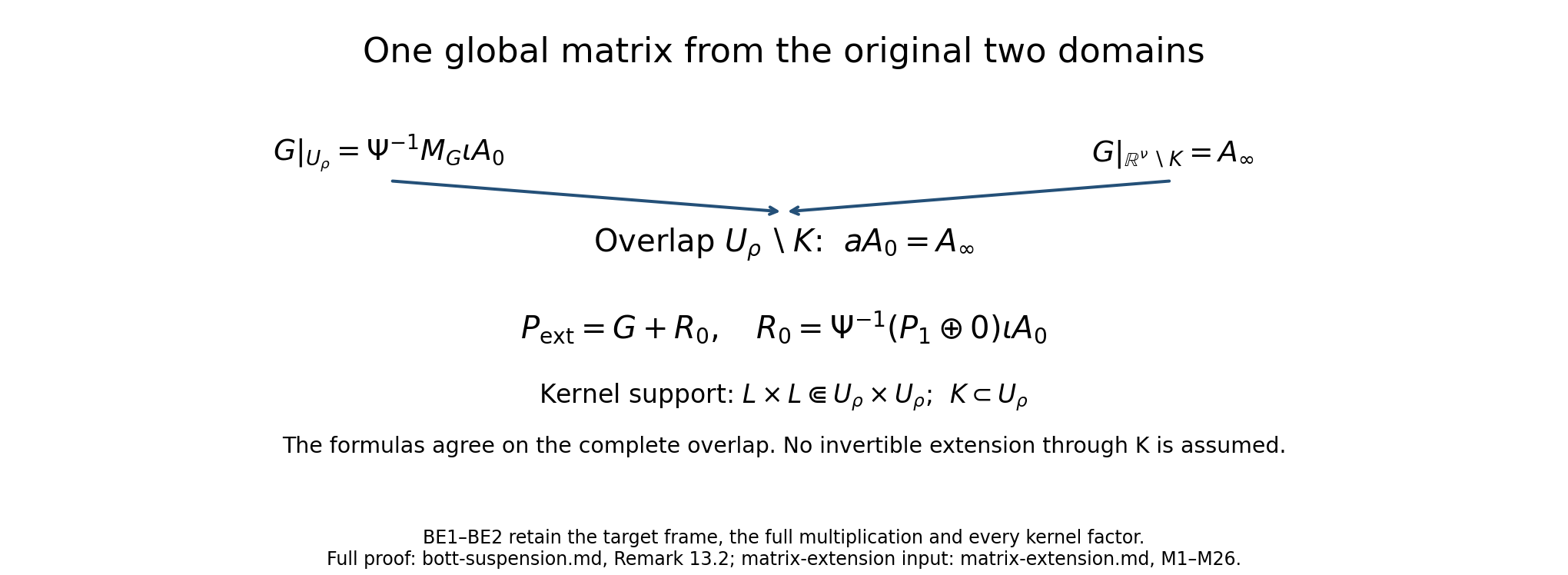
The two restrictions agree on their entire overlap, giving the global map in (BE1). Formula (BE2) retains the full compactly supported kernel. These maps establish the alternate-frame extension in Remark 13.2.
The exact comparison of two extension choices
Retain the matrix , kernel operator and global extension of (BE1)–(BE2). For a second factor pair of the same original , (MG1)–(MG4) in the matrix-extension lesson give a unique smooth invertible map , with and . The letter keeps this globally invertible choice map distinct from the original , which may be singular inside . The unchanged formulas, in their original multiplication order, give The first identity holds on by , and on the exterior by ; these sets cover the full base. For the kernel of , keep its original half-density and both point coordinates: if that matrix kernel is , the new kernel is exactly . Multiplication is at its input point, and the support remains in . Smooth extension by zero therefore retains the same compact support. Adding the two identities proves the last line of (BE3).
On the full original space , multiplication by and by are mutually inverse maps preserving each support exactly. Thus the actual defect maps are Substitution in (BE3) proves both kernel maps and their composites. The range equality follows from the surjectivity of multiplication by ; the quotient map is the identity on that identical range quotient. Hence these choices preserve both original defect dimensions and their difference whenever they are finite. The finite-dimensional assertions and index value remain supplied by the preceding argument, with no additional conclusion inferred from matrix factorization alone.
14. Exercises
Exercise 14.1 (The adjoint model). With and as in Proposition 2.3, show that is injective, has closed range of codimension one, and has index . Identify its cokernel.
Solution. If , then , so , which is in only for . As in (2.2), , so the operator is bounded below and its range is closed. A vector is orthogonal to the range exactly when as a distribution, that is, . So the cokernel is spanned by the Gaussian, and the index is .
Exercise 14.2 (The case ). Using the matrix of for in Example 3.4, verify (3.3) directly. Write as a system acting on , the coefficients of and , and check (4.5) for .
Solution. and in the same way. Replacing by and by (Proposition 3.2(4)), For : , so and . Since , this is . On the other side of (4.5), the degree-two term is , and . The two sides agree.
Exercise 14.3 (Stable complements are stably unique). Let and . Show that .
Solution. , where stands for the trivial bundle and we use associativity and commutativity of the direct sum.
Exercise 14.4 (The homotopy (10.8)). Show that is invertible for and compute . Then consider the degree-one family, in which is evaluated at the vector with real part and imaginary part . It is the analogue of (10.8) with in place of , except that the coefficient of is interpolated geometrically; at the real coefficient is , while the imaginary coefficient is . They agree only if . Show that it is also a family of invertible maps for .
Solution. with and . By (3.3), , with . This is positive: if the first term is positive since ; if , then and the second term is positive since and . The degree-one family has the same form with the positive coefficients and , so the same argument applies.
Exercise 14.5 (The correction term at one point). Let . Evaluate the formula of Example 8.3 with and any with ; the construction of Theorem 7.4 may need smaller values, and these only illustrate the formula. Compute for , compare it with from (7.2), and check that the difference does not change the sign of the real part.
Solution. At , , so ; and , so . Then and . By Example 8.3, The difference is , which is not zero, and the real part stays positive. So alone is not the principal symbol, while the winding (and hence the index) is unchanged.
15. Editorial comparisons on the original graph domain
Reality of the kernel pairing
Corollary 5.5 chooses so that . Convergence alone would only place a complex number near a positive real number. Here the literal scalar symbol is real and even in , so its left operator commutes with complex conjugation: for a real Schwartz function, conjugate its Fourier integral and substitute to recover exactly the same integral. Density extends this commutation to . Bijectivity from Lemma 5.4 then implies that its inverse also commutes with conjugation. The original is real, so the pairing is real. Keeping its original norm and using Lemma 5.4(g), we get for sufficiently small original . This supplies the exact reality step behind the stated choice, rather than altering the Gaussian, its pairing, or the symbol.
An exact strengthening of the full-form upper bound
The upper bound in (4.4) is . For the original full exterior-form space, , its optimal replacement constant is . The weaker original inequality remains true.
Let lie in , and keep and the original norm . The complete comparison, using both (4.2) and (4.3), is Every summand, degree and original norm factor is retained. The final nonnegativity uses precisely and . This proves the stronger bound on the same domain; it makes no change of scale.
It is sharp. Use the original, unscaled Gaussian , of degree . For this input . Integration by parts in gives , and , so the derivative norm is the same. Consequently This nonzero input attains equality in (BS1). The formula holds also for , where the first nonnegative term in (BS1) is zero.
The same stronger upper bound holds on the original even domain of . Its exact parity norm is derived below. The original lower graph estimate, compactness, maximal domain, odd gap and index-one proof remain unchanged. The stronger estimate is an editorial addition to the original oscillator argument.
The exact parity constants are derived below; they strengthen that earlier bounded conclusion on the same domains.
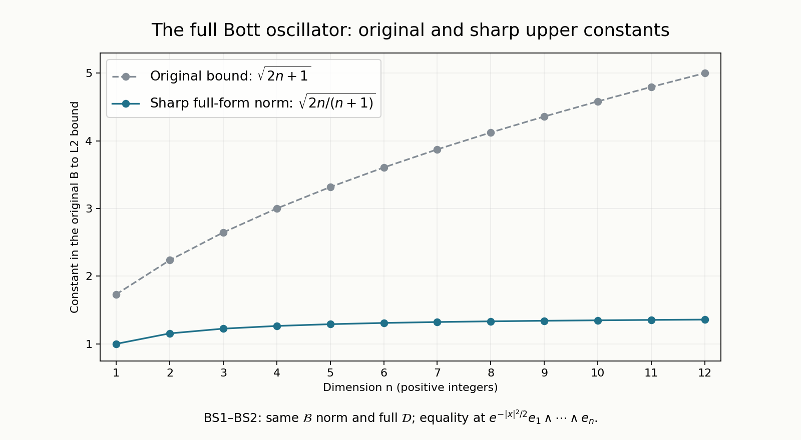
The endpoint description in Exercise 14.4
The displayed degree-one family has real coefficient and imaginary coefficient . Its parenthetical assertion that both coefficients at equal is false for general . The actual endpoints, retaining the original covector norm, are The first two agree precisely when . For example, gives and .
The conclusion of the exercise remains valid. Keep its scalar . Then For both coefficients are strictly positive. If the first term in the square root is positive; if , the second is positive because . The norm formula follows from the original identity , on the original parity spaces. Real-linearity gives , and . Thus the formula, endpoint maps and invertibility proof need no alteration; only the assertion that the two intermediate coefficients agree is removed. This does not change (10.8), Theorem 9.2 or Theorem 13.1.
Sharp constants on the two original parity domains
Let be the set of even degrees or of odd degrees in , with , and let . Keep exactly the original operator , its restricted domain, and its full graph norm. Its norm on that domain is For even input this is the norm of . For odd input it is the norm of the original differential adjoint on ; it is not a claim about the Hilbert adjoint of a map whose domain has the graph inner product.
Here is the complete upper-bound calculation. Write , , and . The exact energy identity in Section 4 gives All coefficients are nonnegative by (BS5). The first equality retains the original , every degree term and the extra in the graph norm. The second uses the same , without a change of scale. The identity extends from Schwartz forms to the full original domain by its already-proved graph density.
If , take , , with the original . Then This attains the bound, including the equality case.
The remaining cases are even input with , and odd input with . The constant is . For any legal degree , take the actual Schwartz inputs , . Since and for , the complete original energy and graph-norm calculation is The coefficient in (BS6) is strictly positive in these two cases, so no nonzero vector attains the constant. The limit proves that no smaller bound is possible. These calculations establish (BS5) for every positive integer , and identify attainment exactly. They sharpen the upper constants only; the kernel, odd lower gap, full principal correction and index proof keep their original formulas and conclusions.
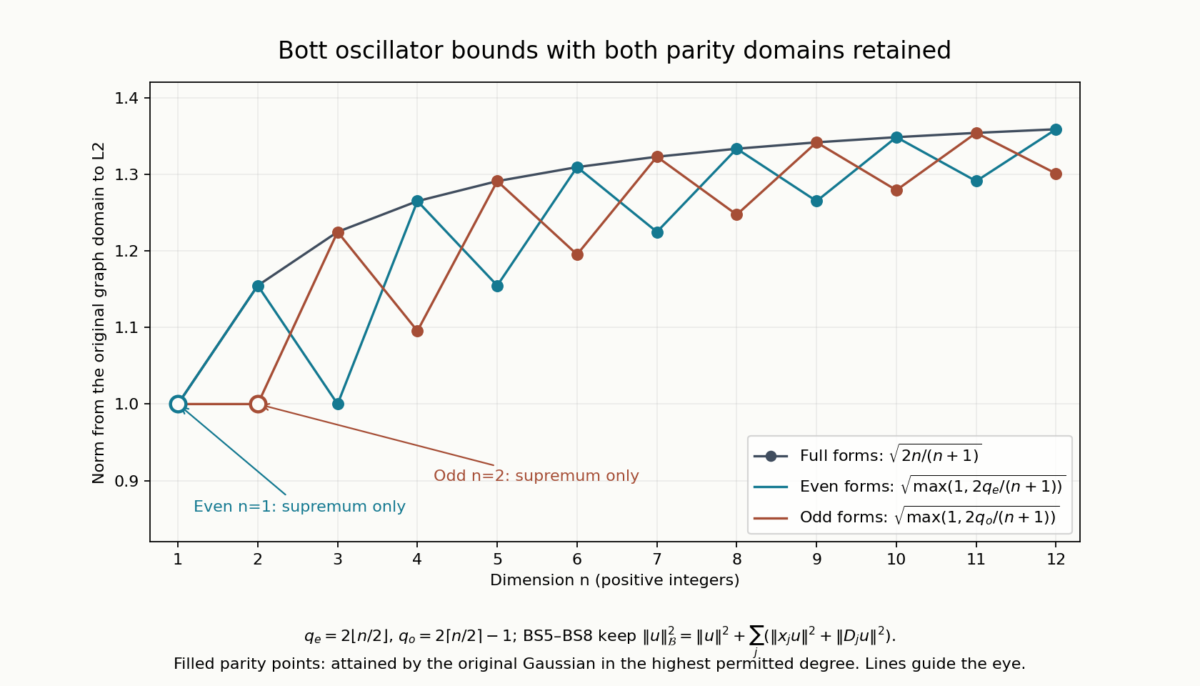
16. Keeping the original symbol through suspension
The degree changes in the suspension proof concern different symbols. This section records the full maps from the original continuous , preserving its values, both vector bundles and the complete suspended block. Let be the union of the positive-dimensional components of . Fix the original cotangent norm , and choose such that the compact exceptional set of over lies in . This disk bundle is compact because is compact.
Write and, for , . For define the first family by The formulas agree at , and . For , and , so the map is invertible. The family is jointly continuous on the entire cotangent bundle: the formula near is the unchanged original symbol. At its exterior value is .
The next family is stationary outside the radius- disk and equals It agrees at . The second summand tends uniformly to zero as , because the original symbol on the radius- sphere is bounded. Thus this family is jointly continuous, and all its possible defects remain in that same disk bundle. Its last member is the degree-one map , where . The full original evaluation and the factor remain explicit.
On the compact unit cosphere is continuous and invertible. The inverse is continuous by the finite-matrix inverse formula in bundle frames, and is bounded. Choose a smooth bundle-map approximation with . Such an approximation is obtained by finite frame charts, a partition of unity and componentwise convolution; uniform continuity controls the error, and compactness controls the transition matrices. Define Continuity at zero follows from the bounded bracket. Its inverse away from zero is the actual ordered expression The series converges uniformly, because its norm ratio is at most . No commuting matrix factors are assumed. The last member is smooth off zero and continuous at zero; it is a different symbol linked by these exact families.
Finally set For every nonzero the displayed scalar is positive. At zero, the whole product is zero and is jointly continuous. The last symbol has degree two. These four families concatenate with their specified endpoints. Every possible defect lies in the same radius- disk bundle, and the original has never been identified with either new symbol.
Here is the receiving map for the full suspension, rather than only its factor index. First join the original extension from (S5) to by their straight line. Both satisfy (9.1), and every intermediate extension does too. For each member of (BQ1)–(BQ4) lift it as Every original weight, real cutoff, positive factor, conjugate adjoint, sign and tensor order is retained. Since and , this lift restricts to on the covectors in (9.1).
If , if , or at the section at infinity, the first factor in this block is invertible by the argument of Theorem 9.2(1). The block lemma therefore applies regardless of the lifted symbol. At the remaining points , write ; then the lifted symbol is exactly . Consequently every defect of every block in (BQ5) lies in the common compact set . The initial extension straight line has the same conclusion. At fibre infinity the diagonal is the identity in the second trivialization, and the lifted off-diagonal maps are continuous; hence joint continuity holds there too.
If the fibre proof selects the cutoff , the additional family retains real values, value one at zero, and vanishes outside the larger of the two fixed radial supports. The preceding block argument applies unchanged. The original can remain fixed throughout. Homotopy invariance now proves, on the original bundles, Section 10 computes the right-hand block index by its actual operator, including both kernel isomorphisms. Combining those equalities proves the conclusion for the original block and original symbol. This comparison does not assert a literal equality of symbols or of their operators.
A zero-dimensional component is a finite set of points and has no cosphere. Keep its original finite-dimensional maps unchanged. Corollary 10.1(2) computes their suspension index by the actual block and the rank difference. A compact manifold has finitely many components; indices and the constructions add over them. This gives the original statement for all components without applying a nonexistent radial construction to a zero-dimensional base component.
Where this leads
- The index formula on Euclidean space. Theorem 13.1 reduces the index of every elliptic operator on a compact manifold to the index of an elliptic system on that equals the identity outside a compact set. For such systems there is an explicit integral formula for the index in terms of the symbol on a large sphere in ; in dimension one it is the winding number of Example 8.3.
- K-theory and characteristic classes. The class of the Bott symbol is the generator in the Bott periodicity theorem, and the suspension theorem is the analytic counterpart of the Thom isomorphism in K-theory. These are the ingredients of the K-theoretic proof of the index theorem. Through them the index is expressed by characteristic classes.
- A first-order operator on the sphere. Step 1 of Section 10 uses the second-order operator . A version with an -invariant first-order operator needs complex powers of elliptic operators.
- Bases that are not compact. Lemma 12.5 extends to every finite-dimensional manifold once one knows that it has a finite trivializing cover; that follows from a covering lemma of dimension theory, which is not proved here.
- Equivariant versions. When a compact group acts on and on the bundles, one can ask for an equivariant reduction. Every construction above except the choice of and of is already -equivariant along the fibres.
17. Editorial prerequisite appendix: exact receiving proofs
The proofs below supply the split-metric composition and elementary foundations used by Facts 1.9 and 1.17–1.20. They use the coordinate, Fourier, support and pairing conventions of Section 1.
17.1. The full split metric in Fact 1.9
Retain , , , and the original positive quadratic form . Write its matrix in these same coordinates as The stated reflection equality gives for every original pair , hence every entry of is zero. The two principal blocks are positive definite. Taking the supremum in the original dual definition, or completing the two independent positive squares, gives Indeed the quotient for a mixed nonzero direction is the weighted mean of these two quotients, with weights its two nonnegative denominator contributions; a pure direction gives each component supremum. Thus follows exactly from . No derivative of a metric matrix is required. Reflection also holds for .
For the two original Bott metrics this gives, without changing their measuring scale, Every factor , , and remains. Their slow-variation and ordered temperateness proofs are the existing Lemma 7.1 and oscillator metric argument; the present receiving map does not alter their hypotheses.
For the actual quantization-change phase , , its symmetric map is The phase-dual supremum therefore gives, in the unchanged original directions, The distance conversion needed for every original ordered metric and weight inequality is An exponent therefore keeps its original constant multiplied by . The factor in a comparison of the phase-dual forms occurs on both sides and remains identifiable before cancellation. Slow variation and local weight continuity use exactly the original . These calculations verify the hypotheses of the preceding Gauss finite-bound theorem (G24)–(G26), with observation space all of , actual phase bound , and counting factor .
Consequently , with , is a continuous map , with bounded-set local smooth continuity. Its remainder of order has target and directional estimate for a finite . The zero phase is : its zeroth remainder is , and all positive-order remainders vanish. The preceding polynomial-growth and bounded compact approximation argument, equations (A3), (A35b), identifies these maps with their distributional Fourier multipliers, so and is the exact inverse. In particular the full maps on the original classes, with coefficient order retained, are The middle map is the preceding Weyl theorem (W31)–(W34), specialized to the same original metric in both factors: its cross parameter is , its product metric is , its diagonal metric is , its actual quadratic phase parameter is , and its derivative comparisons retain , , and the tensor factor . The two conversion phases also have parameter .
The original Weyl multiplier and its restriction are For general symbols this denotes the preceding bounded weak extension. Its product directions have squared length , exactly accounting for the indicated diagonal factor. The tensor product uses the displayed order ; no commutativity of matrix coefficients is assumed.
The preceding operator action (A21) and exact Weyl operator identity (A25), together with the kernel conversion (A36)–(A37), identify (P261.5) with Here the kernel is always the original . Its partial Fourier transform is injective, so the symbol is unique. Each operator has its continuous Schwartz action, making the composite defined on the stated domain.
For the precise remainder required by Fact 1.9, write , , , , and . Then the following is an exact identity, with every ordered term retained: The first term is in by the conversion estimate on the actual weight . The second has that target by the Weyl order-one remainder on the converted inputs. The third and fourth have that target by the full directional product rule. The fifth lies in , whose inclusion into has bound one because the original . Every estimate uses finitely many input seminorms. Products and powers of are legitimate weights: slow variation compares on the same small balls, while , , implies , , and therefore . This proves exactly the target, dependence and domain in Fact 1.9.
17.2. Fact 1.17: inverses, full supports and Green’s formula
The inverse function theorem in the original coordinates. Let be , , , and invertible. The preceding finite-coordinate calculus (OC18)–(OC21a), matrix inversion and completeness give the following direct proof. Choose a closed ball and so that For the unchanged target , define . The segment integral of its derivative proves For , this map takes the closed ball into itself. Its iterates satisfy Coordinate completeness supplies a limit ; continuity gives , hence . Two fixed points agree by (P261.9). Moreover The strict target inequality and (P261.9) put each fixed point inside the open ball. Thus restricts to a bijection between the open set and the displayed open target set , and is continuous.
All in this ball are invertible: has its full convergent Neumann inverse. For and , differentiability of the original gives where the second remainder follows from (P261.10). Therefore , continuously. Induction using the proved coordinate chain rule and smooth matrix inversion gives : if is and , the displayed derivative is , so is . No coordinates or derivative factors were removed. In dimension zero the sole local map and its inverse are the identity on the one point.
Partitions for the entire stated cover. Let be a Hausdorff second countable smooth manifold and any open cover. Every point has coordinate balls with compact closures inside a specified neighborhood: choose two Euclidean balls with nested compact closures inside its chart, and transport the closures back. They remain compact and closed because is Hausdorff. A second countable space has a countable subcover of any open cover: for each basis member contained in some cover member choose one such member; these countably many members cover every point. Thus take a countable family of precompact coordinate balls covering .
Construct compact sets with and . Start with . Given , finitely many precompact balls cover it; let be the union of their closures and . This finite union is compact, contains in its interior, and includes every original eventually. Set all negatively indexed to the empty set. The compact shell lies in the open set . Choose finitely many pairs of coordinate balls , whose smaller members cover , such that The family of larger balls is locally finite. Indeed a point has a neighborhood inside some , and this neighborhood meets no with ; only finitely many balls occur for each remaining .
The preceding cutoff construction in metric foundations Section 5 supplies smooth , equal to one on , with support contained in . Its extension by zero is smooth because that compact support stays inside its coordinate chart. Every point is in some shell, so is positive. Local finiteness makes smooth and gives the same property to The union of any subfamily of the closed supports is closed: near any point only finitely many such sets occur, and their finite union is closed there. Thus The support is a closed set in , exactly as Fact 1.17 requires. Empty members receive zero. On a compact manifold a finite subcover suffices and the same construction can be finite. This justifies sums and extension by zero without weakening the support requirement.
Green’s formula with its original density. In a coordinate chart , keep the Riemannian matrix , its inverse , and . The nonnegative scalar Laplace–Beltrami operator and volume are Take the finite compactly supported chart partition just proved on the compact boundaryless . Componentwise compact integration by parts, with every cutoff term retained, gives The last sum vanishes because its exact covector sum is . Each chart boundary term is zero by compact support, and has no boundary. This is valid without orientability: is a density and the contraction is intrinsic. Summing the same equation over every original vector component gives the stated vector-valued formula. On the Bott sphere the original metric is ; hence , with the coefficient retained.
Keeping a second original smooth function in place of the conjugated in this same calculation gives The identical cutoff cancellation proves both equalities. Thus the formal self-adjointness used for follows with the stated linear-first pairing, rather than from an implicit choice of another adjoint.
17.3. Fact 1.18: the full Hilbert receiver and compact kernel map
For a closed subspace and , let , and choose with . The complete parallelogram identity gives The last square is at least ; thus is Cauchy. Completeness and closedness give a minimizer . Expanding the square for , for real and then purely imaginary , gives for every . Two minimizers agree because their difference lies in and is orthogonal to .
Let be bounded and linear. If , take . Otherwise is closed. For with , its orthogonal component satisfies , and . The inner product is linear in its first variable, so This retains the conjugate. Testing the difference of two representing vectors against itself proves uniqueness. The real Hilbert case omits the conjugate. A functional bounded in the norm on the compact smooth dense subspace extends uniquely by completeness before this representation applies.
The coefficientwise receiver in Lemma 4.3 also retains which test slot is linear. For or , its bound is . This is an antilinear function of the test . Apply (P261.17) to the bounded linear functional , extending it first from . Its representing vector gives the exact conjugate equality For this says that the distribution equals . For , substituting gives , exactly the complex-linear distribution formula for . Thus both required distributions are functions, with the original sign and no change of pairing. Proposition 4.4 uses this same receiver for the maximal domain.
For measurable on , Fubini gives for almost every . Define Cauchy–Schwarz and Fubini retain the entire norm bound Measurability follows by integrable measurable approximations and the preceding product-integration proof (LP3)–(LP4). Values on a null exceptional set may be assigned zero.
The preceding compact smooth density (LP10)–(LP12) approximates by compact smooth functions on the same . Uniform continuity on a compact box then gives finite rectangular-grid approximants where are bounded boxes. The uniform error times the square root of the full box volume bounds its error. Each associated operator has range in , and (P261.18) gives . Its unit-ball image is totally bounded: use a finite net for the bounded finite-dimensional image and this uniform approximation. Completeness makes its closure compact. Finite rectangular matrix kernels keep every entry and intermediate index sum, and the same proof applies to the corresponding finite Hilbert direct sums.
In Section 13 the actual support has finite volume, and the retained decay gives The substitution has absolute Jacobian one, and all finite matrix entries obey the same estimate. Thus compactness keeps the actual one-sided support and requires no unsupported assertion that this error kernel is supported in .
17.4. Fact 1.19: convergence and uniform compactness
Dominated convergence is the preceding proof (LP1)–(LP2) in Banach foundations Section 15.1, extended to general measures in Section 16.1. If measurable complex almost everywhere and for an integrable nonnegative , then off the same null set. Fatou’s inequality applied to the full nonnegative function gives The nonnegative error integrals therefore tend to zero, and complex linearity gives . Fatou is proved there from the increasing functions and monotone convergence. This independent proof is the receiver for the Bott frequency integrals and parameter limits.
For Arzelà–Ascoli let be compact metric and uniformly bounded and equicontinuous: for every , one gives for every whenever . Finite covers by balls of radii tending to zero supply a countable dense set . Given a sequence in , successive bounded subsequences at , followed by the diagonal subsequence, give whose values converge at every . Choose the common radius for and finitely many whose balls of smaller radius cover . Once all these finitely many sample differences are below , every satisfies The subsequence is uniformly Cauchy. Scalar completeness and the uniform-limit proof in metric foundations Section 7 give a continuous uniform limit. For a sequence in the closure of , choose approximants in with error at most ; the same argument gives a convergent subsequence. The preceding metric theorem in Section 14.1 converts sequential compactness of that closure to compactness. Empty has the sole zero function; finite-dimensional vector values use their full coordinate subsequences.
For Lemma 7.2 the near-part supports remain and . The stated common bounds on imply the common equicontinuity on the closed ball by the segment estimate. Uniform convergence gives convergence by the original support makes the exterior contribution zero.
17.5. Fact 1.20: every zero-gradient distribution is constant
Keep the complex-linear distribution pairing, the connected open , and a box with compact closure in . Choose with , and set . For let and define the complete original primitives The bracket has integral zero over , so its primitive vanishes near both endpoints. Its remaining supports are compact and the preceding coordinates have their compact factors. Compact differentiation under the integral, proved in the preceding calculus/integration providers, gives . Differentiating and summing retains every marginal term and telescopes: If , the exact derivative convention therefore gives Intersecting boxes have the same constant: test with a compact smooth function of integral one in their nonempty open intersection. The points reachable from a fixed point by finitely many intersecting boxes form an open set whose complement is open by the local box argument. Connectedness makes this set all of . Hence one constant works on every box. For any compactly supported test, finitely many boxes cover its support. The partition proof above splits it into finitely many box tests; summing gives This proves equality with the original constant-function distribution, retaining all derivative signs. In dimension zero the connected nonempty domain is the one point and its test space is one-dimensional, so every distribution is its constant distribution. The empty domain has its unique zero distribution.
The receivers in this lesson keep the original exponential coefficients. In Proposition 2.3, gives . In Proposition 4.4, for the original , gives . The distribution product rule follows directly by applying its derivative definition to the product of the test function and the smooth multiplier. These multipliers and their inverses are smooth on every compact test support, so no global growth condition is inserted into their distribution multiplication.
References
The proof inputs are the earlier course lessons linked in Section 1. The receiving arguments are written out in this lesson:
- Split-metric composition, (P261.1)–(P261.7).
- Inverses, subordinate partitions and Green’s formula, (P261.8)–(P261.15).
- Hilbert representation and compact kernels, (P261.16)–(P261.20).
- Dominated convergence and uniform compactness, (P261.21)–(P261.23).
- Zero-gradient distributions, (P261.24)–(P261.27).
- Matrix extension and the comparison of frame choices, (M1)–(M26) and (MG1)–(MG4); the ordered receiving maps are (BE1)–(BE4) in Remark 13.2.