Boundary wave fronts for elliptic systems

For an elliptic boundary problem, a boundary singularity of the solution is exactly a singularity of the interior forcing or of one of the boundary measurements. Proving that equality requires two different regularity gains. Before traces are available, the normal equation moves one unit from the tangential weight into the total-frequency weight. Once the trace threshold is reached, the generalized boundary parametrix raises total-frequency regularity while keeping the tangential weight fixed.

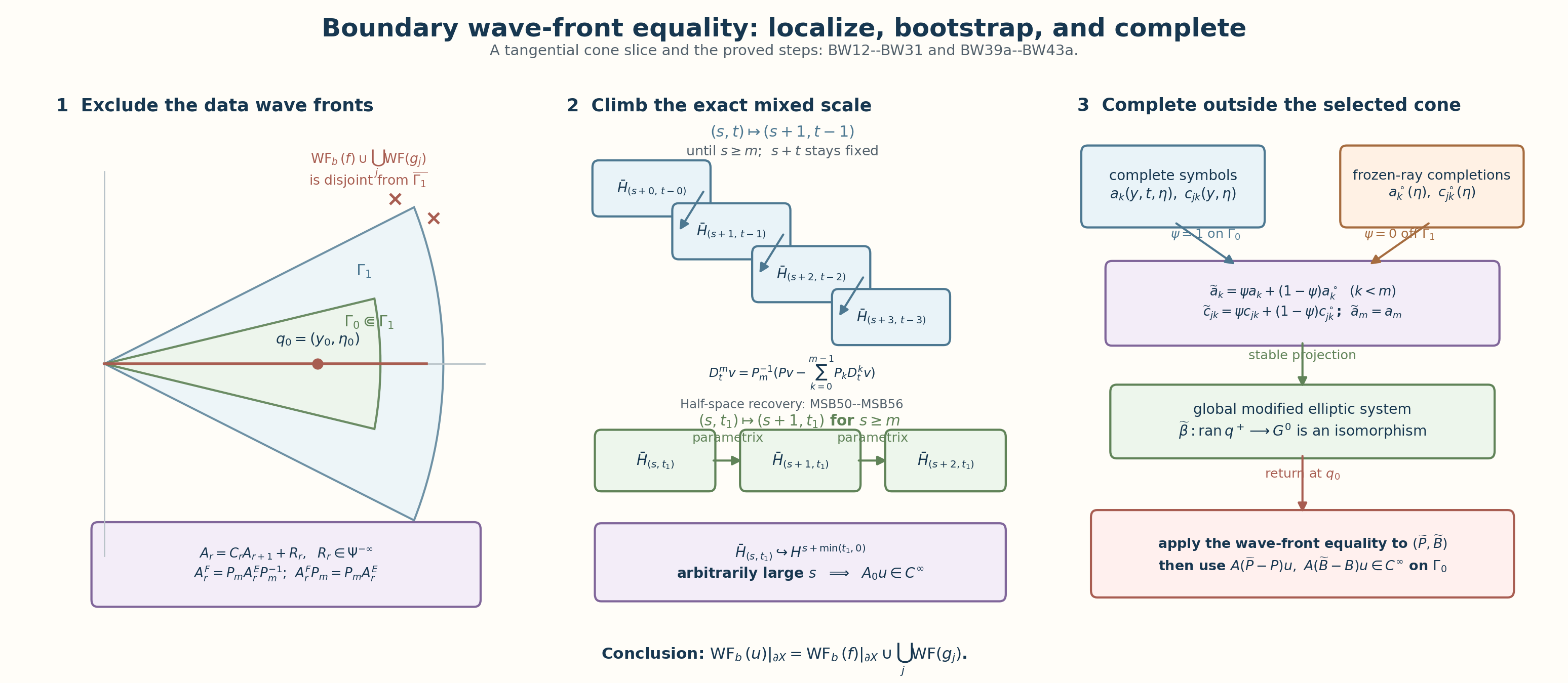
This lesson proves the equality with all normal powers and both Sobolev exponents visible. It then defines the local characteristic set for a differential boundary problem, deletes only redundant boundary output coordinates, completes the coefficients outside a selected tangential cone, and proves the local microlocal inclusion. The final section separates two doubling-index conventions by exact block-sum algebra.

Named prerequisites are Global boundary calculus on the compressed cotangent bundle, Sobolev mapping with normal and tangential weights, and Fredholm boundary problems with first-order Calderón defects. The proof uses their tangential tester, two-weight mapping theorem, trace theorem, and local generalized parametrix with the hypotheses stated there.

Throughout, $D=-i\partial$. Matrix factors keep their displayed order. Every wave-front statement is local in a product collar and is invariant under the bundle and compressed-cotangent coordinate maps proved in the first named prerequisite.

1. The boundary class and the original system

Let $\mathcal A(X)$ and $\mathcal A'(X)$ be the conormal test and dual classes from Global boundary calculus on the compressed cotangent bundle. Embed $T^*\partial X\setminus0$ in the boundary of the compressed cotangent bundle by giving it zero compressed normal component. The noncharacteristic extension class is

$$\mathcal N(X)=\{u\in\mathcal A'(X): \operatorname{WF}_b(u)|_{\partial X} \subset T^*\partial X\setminus0\}. \tag{BW1}$$

Work in a collar $Y\times[0,\varepsilon)_t$. Keep the original generalized elliptic operator $P:E\to F$, its invertible leading normal bundle map $P_m:E\to F$, and the boundary rows in the exact form

$$\begin{aligned} P&=\sum_{k=0}^{m}P_k(t)D_t^k, &P_k(t)&\in\Psi_{\mathrm{tan}}^{m-k}(Y;E,F),\\ P_m(t)&\text{ is multiplication by an invertible bundle map},\\ B_j&=\sum_{k=0}^{m-1}B_{jk}\gamma_k, &B_{jk}&\in\Psi^{m_j-k}(Y;E,G_j), \qquad \gamma_k u=(D_t^ku)|_{t=0}. \end{aligned} \tag{BW2}$$

No identification of $E$ with $F$ is implicit in this formula. The input and output localizers below are related by the exact bundle conjugation $A^F=P_mA^EP_m^{-1}$; thus $A^FP_m=P_mA^E$, with every factor and domain retained. Assume the generalized principal polynomial is elliptic and the principal boundary map is an isomorphism on its stable Cauchy bundle. Let

$$u,f\in\mathcal N(X),\qquad Pu=f\text{ on }X^\circ, \qquad B_ju=g_j\in\mathcal D'(Y,G_j). \tag{BW3}$$

The global theorem below is first proved for a compactly supported collar localization. Proper supports and a finite collar partition then give the stated manifold result.

2. The data cannot have more boundary singularities than the solution

Fix $q\notin\operatorname{WF}_b(u)|_Y$. Choose scalar tangential testers $A_0^E,A_1^E$, acting by scalar symbols in input bundle frames, such that $A_0^E$ is elliptic at $q$, $A_1^E$ has identity symbol on a neighborhood of the microsupport of $A_0^E$, and $A_0^Eu,A_1^Eu$ are smooth. Set $A_0^F=P_mA_0^EP_m^{-1}$. Take both symbols independent of $t$ next to the boundary. Then

$$A_0^FPu=P A_0^Eu+ (A_0^FP-PA_0^E)A_1^Eu+ \sum_{l=0}^{m-1}R_lD_t^lu, \qquad R_l\in\Psi^{-\infty}_{\mathrm{tan}}(E,F). \tag{BW3a}$$

microlocally at $q$. Indeed, expand the commutator by normal power. Its highest coefficient vanishes because $A_0^FP_m=P_mA_0^E$; the lower coefficients and all normal derivatives are given explicitly in (BW15). Each has microsupport in that of $A_0^E$, so the identity region of $A_1^E$ inserts $A_1^E$; the remainder is tangentially smoothing. The first two terms on the right of (BW3a) are smooth because $A_0^Eu$ and $A_1^Eu$ are smooth. Each retained normal jet has the ordinary-normal pseudolocal property proved in GW12. The remainders have no nonzero tangential boundary covector, and the class $\mathcal N(X)$ excludes a residual zero-tangential boundary wave-front point. This proves the required pseudolocal statement with the ordinary normal derivatives retained:

$$\operatorname{WF}_b(f)|_Y =\operatorname{WF}_b(Pu)|_Y \subset\operatorname{WF}_b(u)|_Y. \tag{BW4}$$

Every interior normal jet has the same tangential implication. To see this without treating $D_t$ as a compressed operator, fix $q=(y,\eta)\notin\operatorname{WF}_b(u)|_Y$. The tangential tester theorem in the global boundary calculus lesson supplies a properly supported $A=a(y,t,D_y)$, elliptic at $q$, for which $Au$ is smooth. In its construction take $a$ independent of $t$ near $t=0$. Then for every $k\geq0$, exactly

$$a(y,0,D_y)\gamma_ku=\gamma_k(Au). \tag{BW5}$$

The right side is smooth and the left boundary operator is elliptic at $q$. Its ordinary tangential parametrix proves

$$\operatorname{WF}(\gamma_ku) \subset\operatorname{WF}_b(u)|_Y \qquad(k\geq0). \tag{BW6}$$

Tangential pseudolocality of every $B_{jk}$, with its actual bundle map, now gives

$$\operatorname{WF}(g_j) \subset\bigcup_{k<m}\operatorname{WF}(\gamma_ku) \subset\operatorname{WF}_b(u)|_Y. \tag{BW7}$$

Thus the forcing and all boundary data give the first inclusion in the desired equality.

3. The exact mixed normal-recovery inequality

In a collar chart write

$$R_0(\xi',\xi_n)=(1+|\xi'|^2+\xi_n^2)^{1/2}, \qquad T_0(\xi')=(1+|\xi'|^2)^{1/2}, \tag{BW8}$$

and use the two-weight norm with weight $R_0^sT_0^t$. The elementary inequality that controls the preliminary bootstrap is, for $0\leq j\leq m$,

$$|\xi_n|^jR_0^{s-j+1}T_0^{t-1} \leq 2^{m/2} \left(R_0^sT_0^t +|\xi_n|^mR_0^{s-m+1}T_0^{t-1}\right). \tag{BW9}$$

On $|\xi_n|\leq T_0$, divide the left side by the first term. The quotient is $R_0T_0^{-1}(|\xi_n|/R_0)^j\leq\sqrt2$. On $|\xi_n|\geq T_0$, divide by the second term. The quotient is $(R_0/|\xi_n|)^{m-j}\leq2^{(m-j)/2}$. These two regions prove (BW9), including $j=0$ and $j=m$.

For whole-space inputs, Plancherel applies directly to (BW9). For the actual restriction spaces we instead use the complete half-space argument MSB50–MSB56 in Mixed symbols on every real two-parameter Sobolev scale. It constructs the inverse of $D_t+i\Lambda$, proves uniqueness of its tempered half-space solution, and retains every term of $(D_t+i\Lambda)^mv$. It gives the exact normal-recovery implication

$$v\in\bar H_{(s,t)},\quad D_t^mv\in\bar H_{(s-m+1,t-1)} \Longrightarrow D_t^jv\in\bar H_{(s-j+1,t-1)} \quad(0\leq j\leq m). \tag{BW10}$$

No interpolation endpoint or integer condition on $s,t$ is used.

We shall also use the exact mixed embedding behind every lower normal term. If $0\leq k<m$, a tangential operator of order $m-k$ maps $D_t^kv$, initially in $\bar H_{(s-k,t)}$, into $\bar H_{(s-k,t-m+k)}$. Since $T_0\leq R_0$,

$$\bar H_{(s-k,t-m+k)} \hookrightarrow\bar H_{(s-m+1,t-1)}. \tag{BW11}$$

The quotient of the target weight by the source weight is $(T_0/R_0)^{m-k-1}\leq1$. This keeps both weights and every normal power visible.

4. Admissible tangential localizers and their commutators

Fix $q_0=(y_0,\eta_0)\in T^*Y\setminus0$ outside the boundary wave fronts of $f$ and every $g_j$. Choose nested base-cone neighborhoods

$$V_0\times\Gamma_0\Subset V_1\times\Gamma_1 \Subset\cdots\Subset V_N\times\Gamma_N \tag{BW12}$$

whose largest closure misses those data wave fronts. Because $u,f\in\mathcal N$, the collar may also be chosen so that no relevant boundary wave-front point has $\xi'=0$. Let $A_r^E$ be a scalar, properly supported, order-zero tangential operator in the input bundle, supported in $V_{r+1}\times\Gamma_{r+1}$, elliptic and equal to the identity symbol on $V_r\times\Gamma_r$, with a normal cutoff in the collar. Choose the normal cutoffs nested as well: each outer cutoff is one on a neighborhood of the support of the inner cutoff and all of its normal derivatives. Finitely many such cutoffs exist between two fixed collar neighborhoods by the smooth cutoff construction. Use its scalar boundary symbol on each $G_j$ to define $A_r^{G_j}$, and define $A_r^F=P_mA_r^EP_m^{-1}$. Multiplication by the smooth invertible bundle maps preserves its order, microsupport and scalar principal symbol. For brevity, $A_r$ on an input $u$ means $A_r^E$. Then

$$A_r^Ff\in C^\infty,\qquad A_r^{G_j}g_j\in C^\infty, \qquad A_r=C_rA_{r+1}+R_r,\quad R_r\in\Psi^{-\infty} \tag{BW13}$$

microlocally on $V_r\times\Gamma_r$. The last identity follows by an ordinary tangential parametrix for $A_{r+1}$ on the microsupport of $A_r$; it is the precise meaning of an admissible nested cutoff.

With the domain-correct commutator $\mathcal C_r=PA_r^E-A_r^FP:E\to F$, the original top coefficient in (BW2) gives

$$\mathcal C_r=\sum_{k=0}^{m-1}C_{rk}D_t^k, \qquad C_{rk}\in\Psi_{\mathrm{tan}}^{m-k-1}. \tag{BW14}$$

Here is the complete order check. For a coefficient $P_lD_t^l$,

$$P_lD_t^lA_r^E-A_r^FP_lD_t^l =(P_lA_r^E-A_r^FP_l)D_t^l +P_l\sum_{h=0}^{l-1}\binom lh (D_t^{\,l-h}A_r^E)D_t^h. \tag{BW15}$$

Because $A_r^E$ and $A_r^F$ have the same scalar principal symbol, the leading symbols of $P_lA_r^E$ and $A_r^FP_l$ agree as maps $E\to F$; therefore the first commutator coefficient drops by one tangential order and has order $(m-l)-1$. In the summand with normal power $h<l$, the coefficient has order $m-l\leq m-h-1$. When $l=m$, the first term vanishes because $P_mA_r^E=A_r^FP_m$ exactly, with the original $P_m$ retained. This proves (BW14), including every binomial factor and normal derivative of the localizer.

For the boundary rows put $A_{r,a}^E=(D_t^aA_r^E)|_{t=0}$. Each normal derivative of this tangential family has order zero. The full boundary calculation gives

$$\begin{aligned} \mathcal C_{rj}&=B_jA_r^E-A_r^{G_j}B_j\\ &=\sum_{k=0}^{m-1} (B_{jk}A_{r,0}^E-A_r^{G_j}B_{jk})\gamma_k\\ &\quad+\sum_{k=0}^{m-1}\sum_{a=1}^{k} \binom ka B_{jk}A_{r,a}^E\gamma_{k-a}\\ &=\sum_{k=0}^{m-1}C_{rjk}\gamma_k,\qquad C_{rjk}\in\Psi^{m_j-k-1}(E,G_j). \end{aligned} \tag{BW16}$$

The first sum drops an order because the two localizers have the same scalar principal symbol. In the second sum a coefficient acts on jet $l=k-a$ and has order $m_j-k=m_j-l-a\leq m_j-l-1$. This proves the required bound with all binomial factors, normal derivatives and matrix orders retained. All coefficients in (BW14) and (BW16) have microsupport where $A_{r+1}$ is elliptic. Thus (BW13) inserts $A_{r+1}u$ after each coefficient, modulo a smooth remainder, without changing the displayed orders.

Finally, a compactly supported distribution has finite order. Its Fourier transform grows by a fixed power of $R_0$, so for some real $s_0,t_0$, and hence for the outermost localizer,

$$A_Nu\in\bar H_{(s_0,t_0)}. \tag{BW17}$$

This is only the starting level; no unproved regularity is inserted.

5. Reaching the trace range while preserving the total weight

Assume $A_{r+1}u\in\bar H_{(s,t)}$ and set $v=A_ru$. Equations (BW13)–(BW16) and the mixed mapping theorem give

$$Pv=A_r^Ff+\mathcal C_ru\in\bar H_{(s-m+1,t)}. \tag{BW18}$$

Every lower term $P_kD_t^kv$ belongs to the source space in (BW11), hence to $\bar H_{(s-m+1,t-1)}$. The right side of (BW18) embeds in that same space. Solving the original equation for its highest normal derivative gives

$$D_t^mv=P_m^{-1}\left(Pv-\sum_{k<m}P_kD_t^kv\right) \in\bar H_{(s-m+1,t-1)}. \tag{BW19}$$

The multiplication map $P_m^{-1}:F\to E$ is bounded on these localized mixed spaces by the order-zero mapping theorem. Thus the membership in (BW19) is proved with every original $P_k$ and $P_m$ present. The recovery implication (BW10) now yields the one-step gain

$$A_ru=v\in\bar H_{(s+1,t-1)}. \tag{BW20}$$

The total exponent $s+t$ is unchanged. Starting with (BW17) and using a finite nested family, repeat (BW20) until the first exponent is at least $m$:

$$A_ru\in\bar H_{(s_1,t_1)},\qquad s_1\geq m, \qquad s_1+t_1=s_0+t_0. \tag{BW21}$$

The number of steps is finite even when $s_0$ is not an integer.

6. The boundary parametrix then gains normal order at fixed tangential weight

Suppose now that $A_{r+1}u\in\bar H_{(s,t)}$ with $s\geq m$, and again set $v=A_ru$. The mixed trace theorem gives

$$\gamma_kv\in H^{s+t-k-1/2}(Y,E) \qquad(0\leq k<m). \tag{BW22}$$

Use the boundary equation, with the commutator convention matching (BW16):

$$B_jv=A_r^{G_j}g_j+\mathcal C_{rj}u. \tag{BW23}$$

The first term is smooth. Each term of the second has order $m_j-k-1$ on a trace of order $s+t-k-1/2$. Therefore

$$B_jv\in H^{s+t-m_j+1/2}(Y,G_j). \tag{BW24}$$

Together with (BW18), these are exactly the data spaces for one more first mixed exponent at fixed $t$:

$$Pv\in\bar H_{((s+1)-m,t)},\qquad B_jv\in H^{(s+1)+t-m_j-1/2}. \tag{BW25}$$

Apply the local generalized parametrix proved in Fredholm boundary problems with first-order Calderón defects. Its terms have the unchanged mappings

$$\begin{aligned} V&:\bar H_{((s+1)-m,t)}\longrightarrow\bar H_{(s+1,t)},\\ KS&:\bigoplus_jH^{(s+1)+t-m_j-1/2} \longrightarrow\bar H_{(s+1,t)},\\ \mathscr K&:\bar H_{(s,t)}\longrightarrow\bar H_{(s+1,t)}. \end{aligned} \tag{BW26}$$

The localized identity $v=\mathscr L(Pv,Bv)+\mathscr Kv$ and (BW25)–(BW26) prove

$$A_ru\in\bar H_{(s+1,t)}\qquad(s\geq m). \tag{BW27}$$

For every requested $M$, take a nested family long enough to combine (BW20) up to $s\geq m$ with $M$ uses of (BW27). The innermost localizer is fixed and elliptic at $q_0$. Hence it maps $u$ into $\bar H_{(s,t_1)}$ for arbitrarily large $s$. Since $T_0\leq R_0$, for fixed $t_1$

$$\bar H_{(s,t_1)}\hookrightarrow H^{s+\min(t_1,0)}, \tag{BW28}$$

so local Sobolev embedding at arbitrarily large order proves

$$A_0u\in C^\infty(X). \tag{BW29}$$

By the tangential tester theorem, $q_0\notin\operatorname{WF}_b(u)|_Y$. This closes every normal-derivative, boundary-commutator, and nonintegral-exponent step in the reverse inclusion.

7. Boundary wave-front equality for a generalized elliptic problem

The argument in Sections 4–6 applies at every covector outside the forcing and boundary-data wave fronts. It proves

$$\operatorname{WF}_b(u)|_Y \subset\operatorname{WF}_b(f)|_Y \cup\bigcup_j\operatorname{WF}(g_j). \tag{BW30}$$

Combine this with (BW4) and (BW7):

$$\boxed{\operatorname{WF}_b(u)|_{\partial X} =\operatorname{WF}_b(f)|_{\partial X} \cup\bigcup_j\operatorname{WF}(g_j).} \tag{BW31}$$

This proves the boundary wave-front equality with every normal and tangential exponent displayed. The class $\mathcal N(X)$ is essential: it supplies the tangential boundary hyperplane in (BW1), the intrinsic jets in (BW5), and the tangential tester theorem. Nothing here asserts (BW31) for an arbitrary boundary-supported distribution.

8. The local characteristic set for a differential boundary problem

Now let $P:C^\infty(X,E)\to C^\infty(X,F)$ be an arbitrary order-$m$ differential operator between equal-rank complex bundles, with noncharacteristic boundary. In a boundary chart its full homogeneous principal polynomial is

$$\mathfrak p(y,\eta,\tau) =\sum_{k=0}^m p_k(y,\eta)\tau^k, \qquad p_k(y,\lambda\eta)=\lambda^{m-k}p_k(y,\eta). \tag{BW32}$$

For $(y,\eta)\in T^*Y\setminus0$, let $\mathscr M^+_{y,\eta}$ be the finite-dimensional space of bounded solutions on $t\geq0$ of

$$\mathfrak p(y,\eta,D_t)v(t)=0. \tag{BW33}$$

This definition includes polynomial factors multiplying exponentials when a normal root is multiple. Let the principal boundary map be

$$\beta_{y,\eta}:\mathscr M^+_{y,\eta}\longrightarrow \bigoplus_j(G_j)_y,\qquad v\longmapsto\bigl(b_j(y,\eta,D_t)v|_{t=0}\bigr)_j. \tag{BW34}$$

The exact boundary characteristic set is

$$\operatorname{Char}(P;B)= \left\{(y,\eta): \begin{array}{l} \mathfrak p(y,\eta,\tau)\text{ is singular for some }\tau\in\mathbb R, \text{ or}\\ \beta_{y,\eta}\text{ is not injective} \end{array}\right\}. \tag{BW35}$$

The definition uses injectivity. Surjectivity is neither inserted nor needed when the original boundary list contains redundant equations.

9. Completing the system outside a narrow tangential cone

Fix $q_0=(y_0,\eta_0)\notin\operatorname{Char}(P;B)$. Put $d=\dim\mathscr M^+_{q_0}$. In local frames the matrix of $\beta_{q_0}$ has column rank $d$, so some $d\times d$ minor is nonzero. Retain exactly those $d$ output components. Their boundary map

$$\beta^0_{q_0}:\mathscr M^+_{q_0}\longrightarrow G^0_{q_0} \tag{BW36}$$

is an isomorphism. This is a deletion of redundant local output coordinates, not an alteration of the bounded solution space. The discarded equations remain valid data equations but are not needed for the regularity estimate.

Choose conic neighborhoods $\Gamma_0\Subset\Gamma_1$ of the ray $\mathbb R_+\eta_0$, and a smooth degree-zero function $\psi$ for $|\eta|\geq1$, equal to one on $\Gamma_0$ and supported in $\Gamma_1$. Write

$$\eta^\circ(\eta)=\frac{|\eta|}{|\eta_0|}\eta_0. \tag{BW37}$$

Write $a_k(y,t,\eta)$ for a complete classical tangential symbol of the coefficient of $D_t^k$ in $P$, and write $c_{jk}(y,\eta)$ for a complete symbol of the retained coefficient of $\gamma_k$ in $B_j$. Their leading homogeneous terms are the coefficients $p_k$ and $b_{jk}$ used in the principal polynomial and principal boundary map. This distinction matters below: extending only $p_k$ and $b_{jk}$ would leave the lower-order operator terms uncontrolled.

Retain the original leading normal coefficient. For $k<m$ set

$$\widetilde p_k(y,t,\eta) =\psi(\eta)p_k(y,t,\eta) +(1-\psi(\eta))p_k(y_0,0,\eta^\circ(\eta)), \qquad \widetilde p_m=p_m(y,t). \tag{BW38}$$

At bounded $|\eta|$, join these formulas by a smooth cutoff; that changes only low tangential frequencies. For each retained boundary component and $k<m$, use the matching formula

$$\widetilde b_{jk}(y,\eta) =\psi(\eta)b_{jk}(y,\eta) +(1-\psi(\eta))b_{jk}(y_0,\eta^\circ(\eta)). \tag{BW39}$$

Choose classical symbols $a_k^\circ(\eta)$ and $c_{jk}^\circ(\eta)$ whose leading homogeneous terms are respectively the frozen terms in (BW38) and (BW39), using fixed smooth completions at bounded $|\eta|$. Define the complete modified symbols, in the same local frames and with left quantization, by

$$\begin{aligned} \widetilde a_k &=\psi a_k+(1-\psi)a_k^\circ &&(0\leq k<m), &\widetilde a_m&=a_m,\\ \widetilde c_{jk} &=\psi c_{jk}+(1-\psi)c_{jk}^\circ &&(0\leq k<m). \end{aligned} \tag{BW39a}$$

Take $\psi=1$ on a full base-cone neighborhood of the later localizer’s microsupport, and quantize (BW39a) with proper supports. The bounded-frequency completions change the operators by tangentially smoothing terms. Equations (BW38), (BW39), and (BW39a) therefore retain every normal power, every homogeneous principal coefficient, every lower-order coefficient, the leading normal map, and the displayed matrix order.

We now prove ellipticity rather than infer it from the formula. On the normalized ray $|\eta|=1$, choose $L$ so large that invertibility of the leading normal coefficient gives

$$\|\mathfrak p(y_0,\widehat\eta_0,\tau)z\| \geq c(1+|\tau|)^m\|z\| \qquad(|\tau|\geq L). \tag{BW40}$$

On the compact interval $|\tau|\leq L$, absence of a real characteristic root gives a positive minimum singular value. Shrink the base collar and $\Gamma_1$ until every normalized coefficient polynomial there is closer than half that minimum to the frozen-ray polynomial. Every convex combination in (BW38) is then equally close to the frozen polynomial. Together with (BW40), homogeneity proves that the modified polynomial is elliptic for every nonzero real $(\eta,\tau)$.

For the boundary condition, first fix the Douglis–Nirenberg order reductions

$$S_{\mathrm{in}}(\eta)(v_0,\ldots,v_{m-1}) =(v_0,|\eta|^{-1}v_1,\ldots,|\eta|^{-(m-1)}v_{m-1}), \qquad S_{\mathrm{out}}(\eta)(w_j)_j=(|\eta|^{-m_j}w_j)_j. \tag{BW40a}$$

They turn the graded principal boundary map into an order-zero map on the tangential cosphere. All singular values below are those of this reduced map in fixed bundle metrics. Now write the correspondingly reduced normal polynomial as its first-order companion matrix $\mathcal C(y,\eta)$. Ellipticity keeps its spectrum away from the real axis. A fixed contour surrounding the stable half-plane spectrum gives the stable projection

$$q^+(y,\eta)=\frac1{2\pi i}\int_{\mathscr C} (z-\mathcal C(y,\eta))^{-1}\,dz. \tag{BW41}$$

The resolvent identity makes (BW41) continuous in all normalized coefficients. Its range has the constant dimension $d$. The least singular value of (BW36) is positive; after the same shrinking, the retained modified boundary map stays within half that value. Hence

$$\widetilde\beta_{y,\eta}: \operatorname{ran}q^+(y,\eta)\longrightarrow G^0_y \quad\text{is an isomorphism} \tag{BW42}$$

for every nonzero tangential covector of the modified collar problem. Thus (BW38)–(BW39a) define a generalized elliptic boundary problem to which (BW31) applies.

We now prove the microlocal comparison at complete-symbol level. Choose an order-zero tangential localizer $A$, elliptic at $q_0$, whose full microsupport lies in the base-cone region where $\psi=1$. Since $1-\psi$, with all of its derivatives, vanishes on a neighborhood of that microsupport, the full ordered composition formula gives

$$\begin{aligned} A(\widetilde P-P)&=\sum_{k=0}^{m-1}R_kD_t^k, &R_k&\in\Psi_{\mathrm{tan}}^{-\infty},\\ A(\widetilde B_j-B_j)&=\sum_{k=0}^{m-1}S_{jk}\gamma_k, &S_{jk}&\in\Psi^{-\infty}(Y). \end{aligned} \tag{BW43}$$

This formula retains the normal powers; no principal-symbol agreement is being used as a substitute for a complete-symbol statement. To check its action on the declared domain, put $w_k=D_t^ku$. Ordinary normal pseudolocality from (GW12) gives $w_k\in\mathcal A'$ and $\operatorname{WF}_b(w_k)\subset\operatorname{WF}_b(u)$. Each $R_kw_k$ remains in $\mathcal A'$. Its nonzero tangential boundary wave front is empty because $R_k$ is tangentially smoothing, and its pure-normal boundary wave front is empty because $u\in\mathcal N(X)$. After shrinking the normal cutoff once, closedness of the compressed wave-front set excludes interior points approaching this compact boundary support. Equation (GW8) then puts $R_kw_k$ in $\mathcal A$, and the proved identity $\mathcal A'\cap\mathcal A=C^\infty$ makes it smooth. On the boundary, each $S_{jk}$ maps the distribution $\gamma_ku$ to a smooth section. Hence, on the smaller collar,

$$A(\widetilde P-P)u\in C^\infty,\qquad A(\widetilde B_j-B_j)u\in C^\infty. \tag{BW43a}$$

Consequently the modified data satisfy, microlocally at $q_0$,

$$\widetilde Pu=f+(\widetilde P-P)u,\qquad \widetilde B_ju=g_j+(\widetilde B_j-B_j)u, \tag{BW44}$$

and have no wave-front point at $q_0$ whenever the original data do not. Apply (BW31) to the modified system and use (BW43a):

$$\boxed{\operatorname{WF}_b(u)|_{\partial X} \subset\operatorname{Char}(P;B) \cup\operatorname{WF}_b(f)|_{\partial X} \cup\bigcup_j\operatorname{WF}(g_j).} \tag{BW45}$$

The proof is local. Extend the frozen coefficients outside the chosen base patch and use proper cutoffs; the coefficient family remains in the same small neighborhood used in (BW40)–(BW42), while separated support errors are smooth. The intrinsic compressed coordinate law and bundle conjugation then prove (BW45) on any smooth manifold with boundary. Compactness and global ellipticity of the original problem were never assumed. Equations (BW35)–(BW45) prove the local theorem without compactness or a globally elliptic original problem.

10. What the two doubling index statements can mean

Let $A$ be a Fredholm realization of a boundary problem and let $C$ be the realization placed on the complementary half of a doubled construction. Suppose a doubled realization $D$, after fixed domain and target trivializations, is joined through a continuous Fredholm path to $A\oplus C$. Direct conjugation to the block sum is the constant-path special case. Homotopy invariance and the exact splitting of the endpoint kernel and cokernel give

$$\operatorname{ind}D =\operatorname{ind}A+\operatorname{ind}C. \tag{BW46}$$

There are two distinct specializations:

$$\begin{array}{lll} \operatorname{ind}C=0 &\Longrightarrow& \operatorname{ind}D=\operatorname{ind}A,\\[2mm] \operatorname{ind}C=\operatorname{ind}A &\Longrightarrow& \operatorname{ind}A=\dfrac12\operatorname{ind}D. \end{array} \tag{BW47}$$

Doubling a boundary problem and computing its index constructs the fixed-domain coupling path. Its complementary half is the reflected split model, whose boundary realization has index zero. For that concrete geometric double,

$$\operatorname{ind}(P,B)=\operatorname{ind}\widehat P =\operatorname{sind}(\widehat p). \tag{BW47a}$$

Thus the equality statement and the one-half statement belong to different strata of doubled data. Formula (BW47a) is the geometric zero-index-complement formula. A one-half formula is valid only after a separately specified complement is proved to have the same index as the original realization. The introductory one-half wording is therefore underdetermined for $\widehat P$; it cannot replace (BW47a). The named lesson supplies the operator, bundles, trace domain, coupling, and norm-limit symbol-index proof.

11. A scalar check

For the scalar Laplacian in the half-space,

$$\mathfrak p(\eta,\tau)=|\eta|^2+\tau^2,\qquad \mathscr M^+_{\eta}=\operatorname{span}\{e^{-t|\eta|}\}. \tag{BW48}$$

Dirichlet data give $\beta_\eta(e^{-t|\eta|})=1$. With $D_t=-i\partial_t$, Neumann data give $\beta_\eta(e^{-t|\eta|})=i|\eta|$. Both are nonzero for $\eta\ne0$, so $\operatorname{Char}(P;B)$ is empty for either scalar boundary problem. Formula (BW45) then reduces to the exact boundary wave-front control in (BW31). This check detects the sign of $D_t$, the exclusion of the zero covector, and the use of injectivity in (BW35).

12. Exercises with complete solutions

Exercise 1. Prove the mixed normal-recovery inequality

Let $0\leq j\leq m$, $R_0=(1+|\xi'|^2+\xi_n^2)^{1/2}$, and $T_0=(1+|\xi'|^2)^{1/2}$. Prove (BW9) without assuming that either Sobolev exponent is an integer.

Solution. If $|\xi_n|\leq T_0$, divide the left side of (BW9) by $R_0^sT_0^t$. The quotient is

$$\frac{R_0}{T_0}\left(\frac{|\xi_n|}{R_0}\right)^j \leq \sqrt2. \tag{BW49}$$

If $|\xi_n|\geq T_0$, divide by $|\xi_n|^mR_0^{s-m+1}T_0^{t-1}$. The quotient is $(R_0/|\xi_n|)^{m-j}\leq2^{(m-j)/2}$. Both bounds are at most $2^{m/2}$ for $m\geq1$. The powers $R_0^sT_0^t$ cancel before either estimate, so the proof holds for all real $s,t$.

Exercise 2. Recover every commutator order

Assume $P_l:E\to F$ has tangential order $m-l$, $P_m$ is an invertible multiplication map, and $A^E$ has scalar order-zero principal symbol. Put $A^F=P_mA^EP_m^{-1}$. Prove that the coefficient of $D_t^h$ in $PA^E-A^FP$ has tangential order at most $m-h-1$.

Solution. For the term with normal power $l$, the exact expansion is

$$P_lD_t^lA^E-A^FP_lD_t^l =(P_lA^E-A^FP_l)D_t^l +P_l\sum_{h=0}^{l-1}\binom lh(D_t^{l-h}A^E)D_t^h. \tag{BW50}$$

The two localizers have the same scalar principal symbol, so the leading symbols of $P_lA^E$ and $A^FP_l$ cancel. For $l<m$ their difference has order at most $m-l-1$. In the sum, the coefficient of $D_t^h$ has order $m-l\leq m-h-1$ because $h<l$. For $l=m$, the original leading map remains present and $P_mA^E-A^FP_m=0$ exactly. Summing over $l$ gives (BW14), with every matrix factor in its displayed order.

Exercise 3. Check the fixed-weight boundary gain

Suppose $v\in\bar H_{(s,t)}$ with $s\geq m$, and $C_{jk}\in\Psi^{m_j-k-1}$. Show that $C_{jk}\gamma_kv\in H^{s+t-m_j+1/2}$, the boundary space required for a solution in $\bar H_{(s+1,t)}$.

Solution. The mixed trace theorem gives $\gamma_kv\in H^{s+t-k-1/2}$. Applying an operator of order $m_j-k-1$ lowers this exponent by exactly that amount:

$$s+t-k-\frac12-(m_j-k-1) =s+t-m_j+\frac12 =(s+1)+t-m_j-\frac12. \tag{BW51}$$

This is the boundary target exponent for the $(s+1,t)$ parametrix. The condition $s\geq m$ ensures every trace with $0\leq k<m$ exists.

Exercise 4. Justify the retained boundary coordinates

Let $\beta:M\to G$ be injective with $\dim M=d<\infty$. Prove that one may retain $d$ output coordinates so that the resulting map is an isomorphism, and prove that this property persists under sufficiently small normalized coefficient changes.

Solution. In bases, the matrix of $\beta$ has column rank $d$. Therefore at least one $d\times d$ minor has nonzero determinant. Projection onto those $d$ output coordinates gives a square injective map $\beta^0:M\to G^0$, hence an isomorphism. After the reductions (BW40a), let $\sigma_{\min}>0$ be its least singular value. If a reduced map $\widetilde\beta$ satisfies

$$\|\widetilde\beta-\beta^0\|<\sigma_{\min}, \tag{BW52}$$

then $\|\widetilde\beta v\|\geq (\sigma_{\min}-\|\widetilde\beta-\beta^0\|)\|v\|>0$. It remains injective between equal-dimensional spaces and is therefore an isomorphism. The Riesz projection (BW41) identifies the nearby stable spaces continuously, so the estimate applies to the completed boundary map.

Exercise 5. Distinguish the two doubled indices

Let a doubled realization $D$ be joined through a fixed-space Fredholm path to $A\oplus C$. Compute its index when $C$ has index zero and when $C$ has the same index as $A$.

Solution. Kernels and cokernels split under a block sum, and the index is constant on the Fredholm path. Therefore

$$\operatorname{ind}D=\operatorname{ind}A+ \operatorname{ind}C =\begin{cases} \operatorname{ind}A,&\operatorname{ind}C=0,\\[1mm] 2\operatorname{ind}A,&\operatorname{ind}C=\operatorname{ind}A. \end{cases} \tag{BW53}$$

The first construction yields equality with the doubled index. The second yields one half of it. One may select a line only after proving which complementary realization the concrete doubling uses.

13. Reading notes and references

The three named prerequisites at the start contain complete proofs of the compressed tangential tester, the two-weight operator estimates, the mixed trace theorem, and the generalized collar parametrix used here. The present lesson proves (BW1)–(BW53) directly from those results and keeps the original normal powers, coefficient matrices, boundary-row orders, and Sobolev exponents.

Gerd Grubb, “Fractional Laplacians on domains, a development of Hörmander’s theory of μ-transmission pseudodifferential operators,” arXiv:1310.0951v5.

Written and dedicated to the public domain by Codex under CC0 1.0.