Reducing arbitrary boundary data to a boundary system

An elliptic interior equation may be paired with boundary measurements that are not elliptic. A reference elliptic boundary problem still gives a precise reduction: the unknown reference data satisfy a pseudodifferential system on the boundary, and regularity or solvability modulo smooth errors for the full problem is equivalent to the corresponding property of that boundary system.

This lesson proves the reduction without assuming that the comparison measurements form an elliptic problem. The reference orders $m_j$ and comparison orders $\mu_k$ remain separate, the full Cauchy trace keeps all $m$ components, and every smoothing term in the two-sided parametrix is retained. Exact equations are distinguished from equations modulo smooth sections.

Start with a measurement that misses a direction. On a cylinder whose cross-section is a two-dimensional torus, prescribe the values on both ends as the reference boundary condition. Instead measure only the derivative in the first torus coordinate. A harmonic mode depending on the second coordinate can have nonzero boundary values and zero measurement. The full compact-cylinder calculation below proves exactly what this loses: higher regularity, smooth-error solvability and closed range. The general reduction then identifies the boundary operator that controls these questions for an arbitrary elliptic reference problem.

The progression is: compute the model; retain the full reference inverse and its errors; derive the comparison system; prove both equivalences; then locate the exact connections to the wider boundary calculus and cotangent-space symbol class. The original general statements and their proofs keep their full order lists and hypotheses.

The named prerequisites are Solving an elliptic system from compatible boundary measurements, Fredholm boundary problems with first-order Calderón defects, Cauchy data from jumps and residues, and The calculus of pseudodifferential operators on a manifold. We use $D=-i\partial$ and restriction Sobolev spaces on a compact smooth manifold with boundary.

A compact cylinder with a missing measurement direction

Take the original coordinates and densities

$$X=\mathbb T^2_y\times[0,1]_t,\qquad y_1,y_2\in\mathbb R/(2\pi\mathbb Z),\qquad d y_1\,d y_2\,dt, \qquad P=D_t^2+D_{y_1}^2+D_{y_2}^2, \qquad D=-i\partial. \tag{CM1}$$

Both bundles are the trivial complex line. Use the full value trace $Bu=(u|_{t=0},u|_{t=1})$ as the reference datum, and the comparison $Cu=(D_{y_1}u|_{t=0},D_{y_1}u|_{t=1})$. Thus the reference orders are $m_0=m_1=0$, the comparison orders are $\mu_0=\mu_1=1$, and the interior order is $m=2$. The two inward normal coordinates are $t$ at the lower end and $1-t$ at the upper end.

For each end $b=0,1$, keep the Fourier convention

$$g_b(y)=\sum_{n\in\mathbb Z^2}g_{b,n}e^{i n\cdot y},\qquad g_{b,n}=(2\pi)^{-2}\int_{\mathbb T^2}g_b(y)e^{-i n\cdot y}\,dy, \qquad \|g_b\|_{H^r(\mathbb T^2)}^2 =(2\pi)^2\sum_n\langle n\rangle^{2r}|g_{b,n}|^2. \tag{CM2}$$

Periodic Fourier and trace foundations. The Euclidean transform in Fourier transforms, finite spectra and convex separation does not by itself establish the periodic series being used here. We supply that step with the original torus density. Direct integration gives $$\int_{\mathbb T^2}e^{i(n-k)\cdot y}\,dy=(2\pi)^2\delta_{nk}. \tag{CF1}$$ For $-\pi\leq z\leq\pi$, set $$F_N(z)=\frac1{N+1}\left|\sum_{k=0}^Ne^{ikz}\right|^2 =\sum_{|k|\leq N}\left(1-\frac{|k|}{N+1}\right)e^{ikz}, \qquad k_N(z_1,z_2)=(2\pi)^{-2}F_N(z_1)F_N(z_2). \tag{CF2}$$ This is nonnegative and has integral one. On $\delta\leq|z|\leq\pi$, the geometric sum gives $F_N(z)\leq((N+1)\sin^2(\delta/2))^{-1}$. Translations are continuous in periodic $L^2$: for rectangle indicators the symmetric-difference area tends to zero, then finite rectangle step functions and their $L^2$ density prove the statement for every input. The original measure and step-function density are proved in Banach estimates, quotient spaces and compact parameter arguments. Translation preserves the full torus integral. Cauchy–Schwarz against the probability density $k_N$ now gives $$\|k_N*g-g\|_2^2 \leq\int_{\mathbb T^2}k_N(z)\|g(\,\cdot-z)-g\|_2^2\,dz \leq\varepsilon^2+ \frac{8\|g\|_2^2}{(N+1)\sin^2(\delta/2)} \tag{CF3}$$ once translations with both $|z_j|<\delta$ have difference norm at most $\varepsilon$. The last constant retains the two coordinate tails and the bound $4\|g\|_2^2$ on each translated difference. Thus finite trigonometric polynomials are dense. Orthogonality (CF1) then proves Parseval with factor $(2\pi)^2$, and rectangular Fourier partial sums converge in $L^2$. For every real $r$, define the torus Sobolev norm by (CM2); weighted finite sums are dense in its completion.

Here is its exact connection to the coordinate Sobolev spaces. A smooth cutoff $\chi$ supported in one lifted torus chart satisfies $\widehat{\chi g}(\eta)=\sum_n g_n\widehat\chi(\eta-n)$. The weight inequality is $\langle\eta\rangle^r\langle n\rangle^{-r} \leq2^{|r|/2}\langle\eta-n\rangle^{|r|}$. Put $a_\chi(v)=2^{|r|/2}\langle v\rangle^{|r|}|\widehat\chi(v)|$, $A_\chi=\sup_\eta\sum_n a_\chi(\eta-n)$ and $B_\chi=\int_{\mathbb R^2}a_\chi(v)\,dv$. Both are finite by the Schwartz estimates: subdivide the integral into unit squares, and bound the lattice tails by a convergent power sum. Cauchy–Schwarz first against each kernel row, then summing or integrating the columns, gives $$\|\chi g\|_{H^r(\mathbb R^2)}^2 \leq(2\pi)^{-4}A_\chi B_\chi\|g\|_{H^r(\mathbb T^2)}^2. \tag{CF4}$$ For the converse choose a finite chart partition $\sum_{j=1}^J\chi_j=1$, and a compact smooth $\sigma_j$ equal to one on the support of each lifted $u_j=\chi_jg$. Its Fourier values satisfy $$\begin{aligned} \widehat u_j(n)&=(2\pi)^{-2} \int\widehat\sigma_j(n-\eta)\widehat u_j(\eta)\,d\eta,\\ g_n&=(2\pi)^{-2}\sum_j\widehat u_j(n),\\ \|g\|_{H^r(\mathbb T^2)}^2 &\leq J(2\pi)^{-4}\sum_j A_{\sigma_j}B_{\sigma_j} \|u_j\|_{H^r(\mathbb R^2)}^2. \end{aligned} \tag{CF5}$$ The same row/column estimate proves the last inequality, retaining both convolution and coefficient factors. These identities first hold for smooth inputs and extend by completion; compactly supported distributions also satisfy the convolution identity. They prove the asserted Sobolev identification, including negative $r$.

For the cylinder take the restriction of the product space on $\mathbb T^2\times\mathbb R$, with its full norm $$\|U\|_{H^s}^2=(2\pi)^2(2\pi)^{-1} \sum_n\int_{\mathbb R}(1+|n|^2+\tau^2)^s |\widehat U_n(\tau)|^2\,d\tau, \qquad \widehat U_n(\tau)=\int U_n(t)e^{-it\tau}\,dt. \tag{CF6}$$ The preceding chart argument applies with the same weight inequality uniformly in $\tau$, so this is the coordinate Sobolev space too. For $s>j+1/2$, the $j$-th normal trace at $b=0,1$ is $(2\pi)^{-1}\int e^{ib\tau}(\epsilon_b\tau)^j \widehat U_n(\tau)\,d\tau$, where $\epsilon_0=1$ and $\epsilon_1=-1$. Cauchy–Schwarz and $\tau=\langle n\rangle v$ prove $$\|\gamma_j^{(b)}U\|_{H^{s-j-1/2}(\mathbb T^2)}^2 \leq\frac{J_{s,j}}{2\pi}\|U\|_{H^s}^2,\qquad J_{s,j}=\int_{\mathbb R}v^{2j}(1+v^2)^{-s}\,dv<\infty. \tag{CF7}$$ For each coefficient the integral is continuous in $b$, with the same integrable majorant. An extension vanishing inside the cylinder therefore has zero inward traces. Taking the infimum over extensions proves (CF7) for the restriction space. At integer order two the product Fourier norm is exactly the sum of the squared zeroth derivative norm, twice every first derivative norm, every pure second derivative norm and twice every mixed second derivative norm. The bounded original reflection extension proved in Mixed symbols on every real two-parameter Sobolev scale acts only in $t$, so applies coefficientwise here with all these weights. Equivalently, its order-two endpoint formula is $3u(-t)-2u(-2t)$ at the lower end and $3u(2-t)-2u(3-2t)$ at the upper end, with its retained smooth cutoff. Values and first derivatives match because $3-2=1$ and $-3+4=1$; the full derivative and cutoff estimates of that extension therefore control the restriction $H^2$ norm by the ten derivative norms used below. This completes the periodic foundations of the model.

Put $a=|n|$. The homogeneous solution with both prescribed values is

$$\begin{aligned} (K_0g)_n(t) &=\frac{\sinh(a(1-t))}{\sinh a}g_{0,n} +\frac{\sinh(at)}{\sinh a}g_{1,n},&&a>0,\\ (K_0g)_0(t)&=(1-t)g_{0,0}+t g_{1,0}.&& \end{aligned} \tag{CM3}$$

Direct differentiation gives $-v_n''+a^2v_n=0$ and the exact two endpoint values. The zero mode is retained separately. The full inward first-normal-derivative vector, for $a>0$, is

$$\begin{pmatrix}D_t(K_0g)_n(0)\\D_{1-t}(K_0g)_n(1)\end{pmatrix} =i a\begin{pmatrix}\coth a&-\operatorname{csch}a\\ -\operatorname{csch}a&\coth a\end{pmatrix} \binom{g_{0,n}}{g_{1,n}}, \qquad D_{1-t}=+i\partial_t. \tag{CM4}$$

For $a=0$ the same two derivatives are $(i(g_{0,0}-g_{1,0}),i(g_{1,0}-g_{0,0}))$. These formulas retain the normal signs, the off-diagonal interaction and the constant mode.

Here is a direct completed-space justification. Every nonzero integer frequency $n\in\mathbb Z^2$ in (CM3) has $a=|n|\geq1$. Write

$$p_a(t)=\frac{e^{-at}-e^{-a(2-t)}}{1-e^{-2a}},\qquad p_a^{(j)}(t)= \frac{(-a)^j e^{-at}-a^j e^{-a(2-t)}}{1-e^{-2a}},\quad j=0,1,2. \tag{CM5}$$

The denominator and reflected exponential are both kept. The inequality $|v-w|^2\leq2|v|^2+2|w|^2$ and direct integration give

$$\begin{aligned} \int_0^1|p_a^{(j)}|^2dt &\leq\frac{2a^{2j}}{(1-e^{-2a})^2} \left(\frac{1-e^{-2a}}{2a} +\frac{e^{-2a}-e^{-4a}}{2a}\right)\\ &=a^{2j-1}\frac{1+e^{-2a}}{1-e^{-2a}} \leq (\coth1)a^{2j-1}. \end{aligned} \tag{CM6}$$

There are exactly ten derivatives $\partial_y^\alpha\partial_t^j$ with $|\alpha|+j\leq2$. For each nonzero mode their squared bound has power at most $a^3$. For the zero mode, $1-t$ and $t$ each have the sum of squared zeroth, first and second derivative norms $1/3+1+0=4/3$. Apply the same two-term inequality to the two end contributions and use the full torus Plancherel factor. Then

$$\sum_{|\alpha|+j\leq2} \|\partial_y^\alpha\partial_t^jK_0g\|_{L^2(X)}^2 \leq20(\coth1)(2\pi)^2\sum_n\langle n\rangle^3 (|g_{0,n}|^2+|g_{1,n}|^2). \tag{CM7}$$

Consequently Fourier partial sums converge in $H^2(X)$ for every $g\in H^{3/2}(\mathbb T^2)\oplus H^{3/2}(\mathbb T^2)$. Continuity of the value and normal trace maps in (CF7) passes (CM3)–(CM4) to their proper Sobolev spaces. Also $PK_0g=0$, since $P:H^2\to L^2$ is continuous. A homogeneous $H^2$ solution with zero value traces is zero: its Fourier coefficients satisfy the same one-dimensional equation, and integration by parts yields $\int_0^1(|v_n'|^2+a^2|v_n|^2)dt=0$. At $a=0$ the resulting constant must also have zero endpoint values. This proves uniqueness.

The forcing lift has an equally explicit full kernel. If $t_< =\min(t,r)$ and $t_>=\max(t,r)$, put

$$\begin{aligned} G_a(t,r)&=\frac{\sinh(a t_<)\sinh(a(1-t_>))}{a\sinh a},&&a>0,\\ G_0(t,r)&=t_<(1-t_>),\\ (V_0f)_n(t)&=\int_0^1G_{|n|}(t,r)f_n(r)\,dr. \end{aligned} \tag{CM8}$$

At $t=r$, the jump of $\partial_tG_a$ is minus one: the numerator of that jump is $-\sinh(ar)\cosh(a(1-r))-\cosh(ar)\sinh(a(1-r))=-\sinh a$. The zero-mode jump is also minus one. Thus $(-\partial_t^2+a^2)G_a=\delta_r$, with both Dirichlet values zero. For $a\geq1$, the energy identity and Cauchy–Schwarz give

$$\|v_n\|_2\leq a^{-2}\|f_n\|_2,\qquad \|v_n'\|_2\leq a^{-1}\|f_n\|_2,\qquad \|v_n''\|_2\leq2\|f_n\|_2. \tag{CM9}$$

For example the first bound follows from $a^2\|v_n\|_2^2\leq |(f_n,v_n)|$; inserting it into $\|v_n'\|_2^2+a^2\|v_n\|_2^2=(f_n,v_n)$ proves the second. The equation $v_n''=a^2v_n-f_n$ proves the third. For the zero mode, $\int G_0(t,r)dr=t(1-t)/2\leq1/8$ and the analogous bound in the other variable give the kernel operator norm at most $1/8$ by Cauchy–Schwarz with the nonnegative kernel. The energy identity then gives $\|v_0'\|_2\leq\|f_0\|_2/\sqrt8$, and $v_0''=-f_0$. Each of the ten derivatives used in (CM7) has norm at most $2\|f_n\|_2$ in a nonzero mode; the three nonvanishing zero-mode derivatives obey the stated smaller bounds. Hence

$$\sum_{|\alpha|+j\leq2} \|\partial_y^\alpha\partial_t^j V_0f\|_2^2 \leq40(2\pi)^2\sum_n\|f_n\|_{L^2(0,1)}^2 =40\|f\|_{L^2(X)}^2. \tag{CM10}$$

Smooth Fourier truncation and density pass the kernel equation and zero traces to all $L^2$ inputs. Thus $u=V_0f+K_0g$ is the exact reference inverse at $H^2$, with no remainder for this chosen inverse. The general reference parametrix below keeps its actual smoothing errors.

Since $C$ differentiates only the value traces, this exact reference inverse has reduced boundary operator

$$M_0g=(D_{y_1}g_0,D_{y_1}g_1),\qquad (M_0g)_{b,n}=n_1g_{b,n}. \tag{CM11}$$

For one end and any real $r$, its map is $D_{y_1}:H^r\to H^{r-1}$. Its exact range and closure are

$$\begin{aligned} \operatorname{ran}D_{y_1} &=\left\{h\in H^{r-1}:h_{(0,n_2)}=0\ \text{for all }n_2, \ \sum_{n_1\ne0}\langle n\rangle^{2r} |h_n/n_1|^2<\infty\right\},\\ \overline{\operatorname{ran}D_{y_1}} &=\{h\in H^{r-1}:h_{(0,n_2)}=0\ \text{for all }n_2\}. \end{aligned} \tag{CM12}$$

Necessity follows by taking Fourier coefficients. For sufficiency set $g_n=h_n/n_1$ when $n_1\ne0$, and zero otherwise. The displayed sum puts $g$ in $H^r$ and gives the required image. For the closure, each coefficient is a continuous functional on $H^{r-1}$, whereas finite Fourier sums with $n_1\ne0$ belong to the range and are dense in the displayed subspace. The kernel contains every mode with $n_1=0$, and the target modulo the closure contains every such mode as an independent class.

The range is not closed. Indeed the vectors

$$v_N(y)=\frac{e^{i(y_1+Ny_2)}}{2\pi\langle(1,N)\rangle^r},\qquad \|v_N\|_{H^r}=1,\qquad \|D_{y_1}v_N\|_{H^{r-1}}=\langle(1,N)\rangle^{-1}\longrightarrow0 \tag{CM13}$$

lie in the orthogonal complement of the kernel. A closed range would make the restriction from that complement a bounded bijection onto the range. The Banach inverse theorem, proved in Banach estimates, quotient spaces and compact parameter arguments, would bound these unit vectors by a fixed multiple of their image norms, contradicting (CM13). The same conclusions hold for the two-end direct sum. They also apply to the full comparison problem at its base spaces: $A_B:H^2(X)\to L^2(X)\oplus(H^{3/2}\oplus H^{3/2})$ is a bounded isomorphism with the actual inverse constructed in (CM3)–(CM10). Its zero-Dirichlet forcing lift has zero comparison traces, so $$A_C A_B^{-1}(f,g) =A_C(V_0f+K_0g)=(f,M_0g). \tag{CM15}$$ Thus the kernel of the full map is isomorphic to $\ker M_0$, and its target modulo the closure of its range is isomorphic to the corresponding boundary quotient in (CM12). Its range is not closed, because the product range $L^2(X)\oplus\operatorname{ran}M_0$ is not closed. This gives the exact interior/boundary relation, rather than drawing an inference from the boundary symbol alone.

This also gives actual failures of the two general properties. For $2<s_0\leq s_1$, take

$$g_0(y)=\sum_{N\geq1}N^{-s_0}e^{iNy_2},\qquad g_1=0. \tag{CM14}$$

The squared $H^{3/2}$ sum converges because its large-$N$ power is $3-2s_0<-1$. The $H^{s_0-1/2}$ sum diverges with power minus one. Equation (CM7) gives $u=K_0g\in H^2$, with $Pu=0$ and $Cu=0$. If $u$ belonged to $H^{s_0}$, the value trace theorem would put $g_0$ in the space just shown impossible. Thus $\mathrm{Reg}_X(s_0,s_1)$ fails, as does its boundary counterpart. At $s_0=2$ the regularity assertion is its base hypothesis.

For any $s_1\geq2$, choose the comparison datum $h_0(y)=\sum_{N\geq1}N^{-s_1}e^{iNy_2}$, $h_1=0$, and $f=0$. Its squared target sum in $H^{s_1-3/2}$ has power minus three, so it is admissible. Its coefficients do not decrease faster than every power, so it is not smooth. Every $M_0g$ is zero in these frequencies. Therefore $M_0g-h$ cannot be smooth, for any boundary distribution $g$. Nor can $Cu-h$ be smooth for an interior solution: the same Fourier coefficients of each $D_{y_1}$ trace are zero. Smooth-error solvability fails for the exact comparison problem. These are consequences of the retained measurement and its precise missing frequencies, not a change of interior ellipticity.

1. The reference problem and the comparison measurements

Let $X$ be a compact smooth manifold with boundary $Y$. Let $E,F\to X$ be complex bundles of the same finite rank, and let

$$P:C^\infty(X,E)\longrightarrow C^\infty(X,F) \tag{BDR1}$$

be an elliptic differential operator of order $m\geq1$. Choose an elliptic reference boundary system $\mathbf B=(B_1,\ldots,B_J)$. Its rows have transversal order below $m$ and total orders $m_j$:

$$B_j u=\sum_{r=0}^{m-1}\mathcal B_{jr}\gamma_r u, \qquad \gamma_r u=(D_t^ru)|_Y, \qquad \operatorname{ord}\mathcal B_{jr}\leq m_j-r. \tag{BDR2}$$

The complementing condition is assumed for $(P,\mathbf B)$. The integers $m_j$ need not be below $m$.

Now choose comparison rows $\mathbf C=(C_1,\ldots,C_K)$, with targets $H_k\to Y$, transversal order below $m$, and total orders $\mu_k$:

$$C_k u=\sum_{r=0}^{m-1}\mathcal C_{kr}\gamma_r u =C_k^c\gamma u, \qquad \operatorname{ord}\mathcal C_{kr}\leq\mu_k-r, \qquad \gamma u=(\gamma_0u,\ldots,\gamma_{m-1}u). \tag{BDR3}$$

No complementing condition is imposed on $(P,\mathbf C)$. The problem under study is

$$Pu=f,\qquad C_ku=h_k\quad(1\leq k\leq K), \tag{BDR4}$$

and the auxiliary reference datum will be $g_j=B_ju$.

For every real $s$, put

$$\begin{aligned} \mathcal C^s &=\bigoplus_{r=0}^{m-1}H^{s-r-1/2}(Y,E|_Y),\\ \mathcal D_B^s &=\bigoplus_{j=1}^{J}H^{s-m_j-1/2}(Y,G_j),\\ \mathcal D_C^s &=\bigoplus_{k=1}^{K}H^{s-\mu_k-1/2}(Y,H_k). \end{aligned} \tag{BDR5}$$

Thus $\mathcal B=(\mathcal B_{jr})$ and $C^c=(\mathcal C_{kr})$ have the bounded mappings

$$\mathcal B:\mathcal C^s\longrightarrow\mathcal D_B^s, \qquad C^c:\mathcal C^s\longrightarrow\mathcal D_C^s. \tag{BDR6}$$

These formulas make the two order lists visible. They also cover negative target exponents and arbitrarily large total orders.

2. The complete reference parametrix

Editorial correction of the extension used here. Section 4 of Cauchy data from jumps and residues extends the original operator $P$ elliptically to an open neighborhood $\widehat X$ of $X$. Use that extension and a proper transmission parametrix $T$, on a relatively compact working neighborhood, with

$$TP=I+R_E,\qquad PT=I+R_F, \qquad R_E,R_F\in\Psi^{-\infty}. \tag{BDR7}$$

Let $e^+$ be zero extension and $r^+$ interior restriction. If $P=\sum_{a=0}^mP_aD_t^a$ in the collar, define

$$\begin{aligned} P^cU &=\frac1i\sum_{a=1}^mP_a \sum_{r=0}^{a-1}U_{a-1-r}\otimes D_t^r\delta_0,\\ V&=r^+Te^+, \qquad K=r^+TP^c. \end{aligned} \tag{BDR8}$$

The Calderón operator $Q$ is fixed by the exact trace identity

$$\gamma K=Q,\qquad Q_{r\ell}\in\Psi_{\mathrm{cl}}^{r-\ell},\qquad Q^2-Q\in\Psi^{-\infty}. \tag{BDR9}$$

The complementing condition for $\mathbf B$ gives matrices $S$ and $S''$ with

$$\mathcal BS\equiv I,\qquad QS\equiv S,\qquad S\mathcal B+S''\equiv I,\qquad S''Q\equiv0, \tag{BDR10}$$

where $\equiv$ means equality modulo a matrix with smooth kernel, and

$$S_{rj}\in\Psi_{\mathrm{cl}}^{r-m_j},\qquad S''_{r\ell}\in\Psi_{\mathrm{cl}}^{r-\ell}. \tag{BDR11}$$

Set

$$L_0=(I+KS''\gamma)V,\qquad L(f,g)=L_0f+KSg. \tag{BDR12}$$

At every $s\geq m$, the mapping statements are

$$\begin{aligned} V&:\bar H^{s-m}(X^\circ,F)\longrightarrow\bar H^s(X^\circ,E),\\ S&:\mathcal D_B^s\longrightarrow\mathcal C^s,\\ K&:\mathcal C^s\longrightarrow\bar H^s(X^\circ,E),\\ L&:\bar H^{s-m}(X^\circ,F)\oplus\mathcal D_B^s \longrightarrow\bar H^s(X^\circ,E). \end{aligned} \tag{BDR13}$$

Nothing in (BDR13) evaluates an arbitrary distribution at the boundary: $\gamma$ occurs only after $V$, which has already gained $m$ derivatives.

For $u\in\bar H^m(X^\circ,E)$, the complete left identity is

$$u=L_0Pu+KSBu+\mathcal Ru, \qquad \mathcal R:\bar H^m(X^\circ,E)\longrightarrow C^\infty(X,E). \tag{BDR14}$$

One exact formula retaining the source of this remainder is

$$\mathcal R =K\bigl(\mathcal R_Y\gamma-S''\gamma R_E^+\bigr)-R_E^+, \qquad \mathcal R_Y=I-S\mathcal B-S''(I-Q), \qquad R_E^+=r^+R_Ee^+. \tag{BDR15}$$

Editorial correction of the smoothing argument. The individual summands $I$, $S\mathcal B$ and $S''(I-Q)$ need not be smoothing. The exact regrouping is $$\mathcal R_Y=(I-S\mathcal B-S'')+S''Q. \tag{BDR15a}$$ Both the parenthesized error $I-S\mathcal B-S''$ and the product $S''Q$ have smooth kernels by (BDR10), so their sum $\mathcal R_Y$ has a smooth kernel. Meanwhile $R_E^+$ maps interior $L^2$ inputs continuously to sections smooth up to the boundary. For $u\in\bar H^m$, the trace $\gamma u$ has the stated boundary Sobolev orders, so $\mathcal R_Y\gamma u$ is smooth; $S''\gamma R_E^+u$ is also smooth. The all-order Poisson estimate for $K$, followed by Sobolev embedding at every high order, proves the mapping of $\mathcal R$ in (BDR14), retaining both terms inside $K$ and the final $-R_E^+$. No elliptic extension of the original $P$ to a closed double is required in this proof.

The interior row of the right identity is

$$PL(f,g)=f+K_1f+K_2g, \tag{BDR16}$$

where, with $H=r^+R_FP^c$,

$$K_1=R_F^++HS''\gamma V,\qquad K_2=HS,\qquad R_F^+=r^+R_Fe^+. \tag{BDR17}$$

Both $K_1$ and $K_2$ map their indicated Sobolev inputs continuously into smooth interior sections. In particular, $K_2$ has a kernel smooth in its boundary input and interior output variables.

The reference boundary row is also retained:

$$BL(f,g)=g+K_3f+K_4g, \tag{BDR18}$$

where $K_3:L^2(X,F)\to C^\infty(Y,\bigoplus_jG_j)$ is continuous and $K_4$ has a smooth kernel on $Y\times Y$.

3. The boundary pseudodifferential system

Define the reduced comparison operator

$$M=C^cQS:\mathcal D_B^s\longrightarrow\mathcal D_C^s. \tag{BDR19}$$

Its $(k,j)$ entry has order $\mu_k-m_j$. Indeed every summand has the unreduced order

$$\operatorname{ord}\bigl(\mathcal C_{kr}Q_{r\ell}S_{\ell j}\bigr) \leq(\mu_k-r)+(r-\ell)+(\ell-m_j) =\mu_k-m_j. \tag{BDR20}$$

This calculation keeps all three factors and does not identify $m_j$ with $\mu_k$.

Let $u\in\bar H^m$, put $f=Pu$, $g=Bu$, and $h=Cu$. Apply $C$ to (BDR14). Since $C=C^c\gamma$ and $\gamma K=Q$, one obtains the exact identity

$$C^cQSg =h-CL_0f-C\mathcal Ru. \tag{BDR21}$$

In the original factors this reads

$$C_k^cQSg =h_k-C_k(I+KS''\gamma)Vf-C_k\mathcal Ru, \qquad V=r^+Te^+,\quad K=r^+TP^c. \tag{BDR22}$$

The last term is smooth on $Y$. If $f\in\bar H^{s-m}$, then (BDR13) gives

$$CL_0f\in\mathcal D_C^s. \tag{BDR23}$$

The second identity in (BDR10) gives a smoothing matrix $R_S=QS-S$. Composition with the finite-order row $C^c$ remains smoothing, so

$$M-C^cS=C^c(QS-S)=C^cR_S\in\Psi^{-\infty}. \tag{BDR24}$$

Thus $C^cS$ may replace $M$ in a statement made modulo smooth sections. It may not replace $M$ in an exact equation without also retaining the smoothing correction.

4. The coupled ansatz and its exact scope

For $s\geq m$, take $\widetilde f\in\bar H^{s-m}(X^\circ,F)$, $g\in\mathcal D_B^s$, and set

$$u=L(\widetilde f,g) =(I+KS''\gamma)V\widetilde f+KSg. \tag{BDR25}$$

Equations (BDR16) and (BDR19) give, without suppressing either right error,

$$\begin{aligned} Pu&=\widetilde f+K_1\widetilde f+K_2g,\\ Cu&=CL_0\widetilde f+Mg. \end{aligned} \tag{BDR26}$$

Consequently this particular ansatz solves (BDR4) exactly if and only if its parameters solve the coupled system

$$\boxed{ \begin{aligned} \widetilde f+K_1\widetilde f+K_2g&=f,\\ Mg&=h-CL_0\widetilde f. \end{aligned}} \tag{BDR27}$$

The first equation implies

$$\widetilde f-f=-K_1\widetilde f-K_2g\in C^\infty(X,F). \tag{BDR28}$$

The transmission mapping of $V$, followed by (BDR12), sends a smooth forcing term to a section smooth up to $Y$. Hence

$$CL_0\widetilde f-CL_0f=CL_0(\widetilde f-f)\in C^\infty(Y,\textstyle\bigoplus_kH_k). \tag{BDR29}$$

This is the precise reason that $f$ may replace $\widetilde f$ on the boundary right side modulo smooth terms.

The ansatz does not claim that every exact solution lies in the exact range of $L$. What is true for every solution is the complete modulo-smooth representation

$$u-L(Pu,Bu)=\mathcal Ru\in C^\infty(X,E). \tag{BDR30}$$

Therefore (BDR27) is an exact characterization of solutions produced by the ansatz, while (BDR30) says that the ansatz captures every solution modulo a smooth section. Possible finite-dimensional obstructions in the first equation have not been erased.

The full reference and comparison block

The source’s block notation has a concrete connection to the present maps. Retain the original spaces $\mathcal U^s=\bar H^s(X^\circ,E)$, $\mathcal F^s=\bar H^{s-m}(X^\circ,F)$, and both graded boundary spaces from (BDR5). Write

$$A_B=\binom P B:\mathcal U^s\longrightarrow \mathcal F^s\oplus\mathcal D_B^s, \qquad A_C=\binom P C:\mathcal U^s\longrightarrow \mathcal F^s\oplus\mathcal D_C^s, \qquad L_B=\begin{pmatrix}L_0&KS\end{pmatrix}. \tag{BCM1}$$

All three maps are bounded when $s\geq m$, by (BDR6), (BDR13) and the strict normal trace thresholds. Equations (BDR14), (BDR16) and (BDR18) give the complete products

$$\begin{aligned} L_BA_B&=I-\mathcal R,\\ A_BL_B&=\begin{pmatrix}I+K_1&K_2\\K_3&I+K_4\end{pmatrix},\\ A_CL_B&=\begin{pmatrix}I+K_1&K_2\\CL_0&M\end{pmatrix}, \qquad M=C^cQS. \end{aligned} \tag{BCM2}$$

Each entry has its displayed domain and target; in particular the boundary-input column is retained. Applying the last matrix to $(\widetilde f,g)$ is exactly (BDR27). Applying $L_BA_B=I-\mathcal R$ to an arbitrary $u$ is exactly (BDR30). This proves their connection before taking any quotient by smooth sections. In that quotient the first two products are inverse maps, and the comparison problem becomes the triangular map with rows $(I,0)$ and $(CL_0,M)$; the exact products remain (BCM2).

Melo, Schick and Schrohe, Introduction, equation (1) provide the typed interior/boundary block used for this comparison. Our equation column has zero boundary input bundle; its reference inverse has the actual Poisson column $KS$. Their composition rule is stated for a single order and class. Here the original lists $m_j$ and $\mu_k$ remain separate, and (BDR20) proves the exact order of every entry of $M$. No order-changing substitution or proof of the entire boundary algebra is inferred from (BCM2).

5. Equivalence of regularity gains

Fix real exponents

$$m\leq s_0\leq s_1. \tag{BDR31}$$

Consider the following two assertions.

Interior assertion $\mathrm{Reg}_X(s_0,s_1)$. Every $u\in\bar H^m(X^\circ,E)$ satisfying

$$Pu\in\bar H^{s_1-m}(X^\circ,F), \qquad Cu\in\mathcal D_C^{s_1} \tag{BDR32}$$

belongs to $\bar H^{s_0}(X^\circ,E)$.

Boundary assertion $\mathrm{Reg}_Y(s_0,s_1)$. Every $g\in\mathcal D_B^m$ satisfying

$$Mg=C^cQSg\in\mathcal D_C^{s_1} \tag{BDR33}$$

belongs to $\mathcal D_B^{s_0}$.

Regularity reduction theorem. The two assertions are equivalent.

Assume first $\mathrm{Reg}_X(s_0,s_1)$, and take $g$ as in (BDR33). Put

$$u=KSg. \tag{BDR34}$$

The mappings in (BDR13) put $u$ in $\bar H^m$. Equations (BDR16) and (BDR18), with $f=0$, give

$$Pu=K_2g\in C^\infty(X,F),\qquad Cu=Mg\in\mathcal D_C^{s_1},\qquad Bu=g+K_4g. \tag{BDR35}$$

The interior assertion yields $u\in\bar H^{s_0}$. Therefore $Bu\in\mathcal D_B^{s_0}$; because $K_4g$ is smooth, the last identity in (BDR35) proves

$$g=Bu-K_4g\in\mathcal D_B^{s_0}. \tag{BDR36}$$

This proves $\mathrm{Reg}_Y(s_0,s_1)$.

Conversely assume $\mathrm{Reg}_Y(s_0,s_1)$, and take $u$ as in (BDR32). Set $f=Pu$, $h=Cu$, and $g=Bu$. The trace theorem at the base exponent gives $g\in\mathcal D_B^m$. Equations (BDR21) and (BDR23) imply

$$Mg=h-CL_0f-C\mathcal Ru\in\mathcal D_C^{s_1}. \tag{BDR37}$$

The boundary assertion gives $g\in\mathcal D_B^{s_0}$. Since $s_1\geq s_0$, also $f\in\bar H^{s_0-m}$. Applying (BDR13) to the exact left identity (BDR14) yields

$$u=L(f,g)+\mathcal Ru\in\bar H^{s_0}(X^\circ,E). \tag{BDR38}$$

This proves the converse and the theorem. The final bundle in (BDR38) is $E$, the bundle of the unknown; $F$ is the target of $Pu$.

6. Equivalence of solvability modulo smooth errors

Under (BDR31), consider two more assertions.

Interior assertion $\mathrm{Sol}_X(s_0,s_1)$. For every

$$f\in\bar H^{s_1-m}(X^\circ,F),\qquad h\in\mathcal D_C^{s_1}, \tag{BDR39}$$

there is $u\in\bar H^{s_0}(X^\circ,E)$ such that

$$Pu-f\in C^\infty(X,F),\qquad Cu-h\in C^\infty(Y,\textstyle\bigoplus_kH_k). \tag{BDR40}$$

Boundary assertion $\mathrm{Sol}_Y(s_0,s_1)$. For every $h\in\mathcal D_C^{s_1}$, there is $g\in\mathcal D_B^{s_0}$ such that

$$Mg-h\in C^\infty(Y,\textstyle\bigoplus_kH_k). \tag{BDR41}$$

Smooth-error solvability theorem. The two assertions are equivalent.

Assume $\mathrm{Sol}_Y(s_0,s_1)$. Given $(f,h)$ as in (BDR39), form the interior lift

$$u_f=L_0f=(I+KS''\gamma)Vf\in\bar H^{s_1}(X^\circ,E), \qquad h'=h-Cu_f\in\mathcal D_C^{s_1}. \tag{BDR42}$$

Choose $g\in\mathcal D_B^{s_0}$ with $Mg-h'$ smooth, and set

$$u=u_f+KSg. \tag{BDR43}$$

Since $s_1\geq s_0$, both terms lie in $\bar H^{s_0}$. The two rows of (BDR26) give

$$Pu-f=K_1f+K_2g\in C^\infty(X,F),\qquad Cu-h=Mg-h'\in C^\infty(Y,\textstyle\bigoplus_kH_k). \tag{BDR44}$$

Thus $\mathrm{Sol}_X(s_0,s_1)$ holds.

Conversely assume $\mathrm{Sol}_X(s_0,s_1)$, and fix $h\in\mathcal D_C^{s_1}$. Apply it with $f=0$. There is $u\in\bar H^{s_0}$ such that $Pu$ and $Cu-h$ are smooth. Put

$$g=Bu\in\mathcal D_B^{s_0}. \tag{BDR45}$$

The exact reduction identity (BDR21) now gives

$$Mg-h=(Cu-h)-CL_0(Pu)-C\mathcal Ru \in C^\infty(Y,\textstyle\bigoplus_kH_k). \tag{BDR46}$$

Indeed $Pu$ is smooth, so the all-order mapping of $L_0$ makes $CL_0(Pu)$ smooth; the last term is smooth by (BDR14). This proves $\mathrm{Sol}_Y(s_0,s_1)$.

The theorem asserts solvability modulo smooth errors. It does not assert exact surjectivity, a finite-dimensional cokernel, or a closed range for $(P,\mathbf C)$. Any such conclusion needs an additional theorem connecting smooth-error solvability with the topology of the relevant range.

7. Endpoints, order checks, and a nonelliptic model

At $s_0=m$, the claimed gain in both regularity assertions is exactly their base assumption. At $s_1=s_0$, every occurrence of a Sobolev embedding in the proof becomes the identity map. No strict inequality between the two exponents was used.

For a boundary row of total order $\mu_k$, the trace estimate is

$$\|C_ku\|_{H^{s-\mu_k-1/2}} \leq C\sum_{r=0}^{m-1} \|\gamma_ru\|_{H^{s-r-1/2}}, \qquad s\geq m. \tag{BDR47}$$

This remains valid when $\mu_k\geq m$, because the target exponent is allowed to be negative. The same observation applies independently to every $m_j$.

A frozen scalar model shows why no ellipticity of $\mathbf C$ should be inserted. Let $m=2$, let the tangential covariable be $\eta=(\eta_1,\eta_2)$, and take

$$p(\eta,D_t)=D_t^2+|\eta|^2,\qquad B=\gamma_0,\qquad C=D_{y_1}\gamma_0. \tag{BDR48}$$

For $\eta\ne0$, the decaying normal solution with Dirichlet datum $g$ is $e^{-|\eta|t}g$. Hence the principal reduced boundary operator is

$$\sigma(M)(\eta)g=\eta_1g. \tag{BDR49}$$

It vanishes at every nonzero covector with $\eta_1=0$. The reduction theorem still applies: it identifies regularity and smooth-error solvability of the full comparison problem with those of this nonelliptic tangential operator. It does not manufacture the missing transverse control.

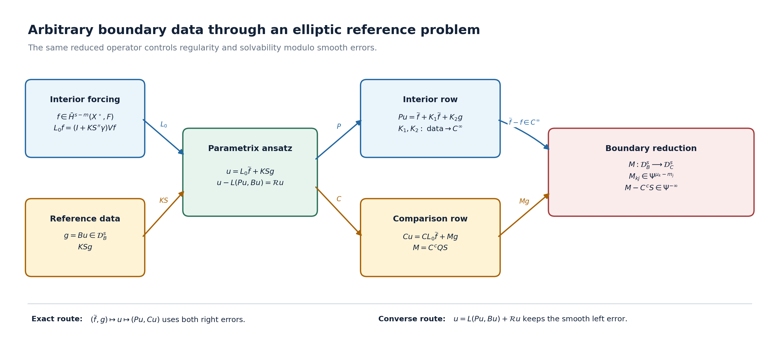
The upper route in the figure is the exact ansatz (BDR25)–(BDR27). The lower route is the left identity (BDR14), which supplies the converse statements modulo its displayed smooth remainder. The two routes meet at the same reduced boundary operator $M$.

8. Exercises with complete solutions

Exercise 1. Verify the order of the $(k,j)$ entry of $C^cS$.

Solution. The $r$-th summand has order

$$\operatorname{ord}(\mathcal C_{kr}S_{rj}) \leq(\mu_k-r)+(r-m_j)=\mu_k-m_j. \tag{BDR50}$$

It therefore maps $H^{s-m_j-1/2}$ to $H^{s-\mu_k-1/2}$, exactly as required.

Exercise 2. Derive (BDR21) without replacing $QS$ by $S$.