Cauchy data from jumps and residues
A boundary value contains several normal derivatives. They form a weighted vector: taking another normal derivative costs one Sobolev order. The central construction below acts on this entire vector. Its leading symbol separates the modes entering the interior from the modes entering the exterior; its full operator is a projection up to a smooth kernel. Establishing that last assertion requires control of distributions at the boundary, beyond a calculation of eigenvalues.
This lesson treats smooth elliptic differential operators of arbitrary positive integer order on complex bundles of arbitrary common finite rank. It neither assumes a scalar factorization nor prescribes the number of boundary equations. The subsequent Fredholm theorem for complementing boundary problems is a separate unit.
The analytic prerequisites are Stable modes and the algebra of boundary data, Sections 1–3, for matrix ODE modes; Singularities along a submanifold and smooth boundary passage, Sections 10–13, for ordinary transmission and all layer traces; and Detecting regularity without choosing coordinates, Sections 5–6, 11 and 13, for properly supported bundle operators, two-sided parametrices and Sobolev bounds. We also use finite-dimensional linear algebra, smooth partitions of unity, Fourier inversion, distributional differentiation, smooth local flows and inverse functions, compactness, and the fundamental theorem of calculus. The projection is constructed directly from these tools; the later boundary Fredholm argument and all-real-order Poisson estimates are separate.
1. The weighted space of boundary jets
Let be a compact smooth manifold with boundary , let be complex smooth bundles of common rank , and let be differential, elliptic, and of order . Ellipticity means that its principal symbol is invertible for every nonzero real covector. Sections here are ordinary bundle sections. Choose a positive smooth density and Hermitian metrics for norms and distributional duality; these choices do not change the operator convention.
Fix an inward collar coordinate and an identification of the bundles in the collar with pullbacks from , constructed in Section 4. Write . The Cauchy vector and its Sobolev space are The space is the space of restrictions of sections on a neighborhood, with quotient norm. In particular . Equivalent finite chart constructions give the same spaces, by Section 11 of Detecting regularity without choosing coordinates.
For completeness the trace estimate needed here is a Fourier calculation. If , Cauchy–Schwarz in the normal frequency gives Indeed the integral of is finite precisely in the indicated range. The substitution gives Editorial restoration of the Fourier factors. In a collar chart of dimension , use the convention , the exact trace formula is For the squared Sobolev norm in dimension , retain the factor . Multiplying (CD3) by and integrating in gives Thus every Fourier factor is present in the trace estimate. For , the tangential integral is over with measure one, so the same calculation gives the point trace. The estimate also makes the trace independent of the extension: a smooth function vanishing on has zero trace there, and approximation in gives the same assertion for an extension difference. One can see the approximation directly by translations away from the boundary followed by convolution, first for compact charts; the Fourier translation factors converge to one and are uniformly bounded. Partitions and bundle frames finish the proof. Thus is continuous for , in particular for every .
The different orders in (CD2) are essential. An entry taking the -th jet to the -th jet must have order to preserve this scale. This statement defines the weight convention we will use; no general theorem about weighted systems is being invoked.
2. Division in the normal derivative
Let , , be boundary differential operators of total orders ; the ranks of the bundles may differ. There are boundary differential operators such that The convention is if . Total order is not reduced to .
Here is a division procedure that retains the order of matrix factors. Locally put , with tangential of order at most . The coefficient is invertible because . If the current boundary operator contains with largest normal exponent , subtract the boundary restriction of . The normal leading term is exactly . Every other term has lower normal order: either it differentiates a coefficient, or it uses with . All terms still have total order at most ; the multiplier of has order at most . Iteration terminates. The inverse matrix occurs to the left of , with the displayed intervening derivatives; it cannot be moved through the other coefficients. Multiply these local identities on the output by a partition of unity on and sum. This proves (CD4) globally without choosing global frames.
For smooth data the equations become exactly At low regularity the expression may itself require traces not defined on . Thus (CD5) is first a smooth-data equivalence. The realization below is for the reduced boundary operators; it does not assert the continuity of an original operator of arbitrarily high normal order at every .
Henceforth write for such a reduced operator. It has the unique collar form where a negative upper bound means that the differential operator is zero. Formula (CD3), followed by tangential differentiation, proves for every the bounded map Large tangential orders are allowed; their targets can be negative Sobolev spaces.
3. The frozen test and its coordinate invariance
At , choose an inward conormal , and choose whose class modulo is nonzero. Let be the space of smooth -valued functions on satisfying and bounded for . A reduced boundary system is complementing when is a bijection. Here is the homogeneous principal symbol of total degree , including zero terms when an actual order is smaller than the assigned order. Injectivity and surjectivity are separate requirements.
The matrix polynomial in (CD8) has invertible leading coefficient. Its determinant has no real zero: for real , , and ellipticity applies. The companion equation and generalized spectral decomposition of Sections 1–3 of Stable modes and the algebra of boundary data therefore split its -dimensional solution space into and . Each component is a finite sum of polynomial factors times ; the positive space uses , and the negative space uses . All derivatives of positive modes decay exponentially as , and conversely a bounded mode has no negative component. This proof includes multiple roots and nontrivial Jordan blocks.
The definition does not depend on the representative . If , then satisfies . The boundary evaluations in (CD9) agree, and boundedness is unchanged. If , , use ; then is the pullback of , and again the maps agree. Tangential coordinate changes transport and all homogeneous symbols by the cotangent map. Frame changes multiply the equation and boundary values by invertible fiber maps. These operations preserve bijectivity. A different normal jet convention produces a triangular invertible transformation on the Cauchy vectors, with the corresponding tangential degrees; it therefore gives the same intrinsic test.
For a smoothly varying nonzero tangential covector, the companion matrix varies smoothly. Locally choose contours separating its upper and lower spectra; the resolvent integral gives smooth projections. These local projections agree by spectral uniqueness, so the stable spaces form bundles over the nonzero tangential cotangent space, homogeneous after the jet rescaling. The earlier formulation said that their ranks “need not be imposed as ”. The exact qualification is dimension dependent: the reflection proof in Section9 forces half rank in dimension at least three. In dimension two the two rays can have different complementary ranks, as the first worked model shows. When , there is no nonzero tangential covector and this microlocal test is empty; the actual boundary Cauchy space is finite dimensional. We do not manufacture a half-rank conclusion in that case.
4. A neighborhood where the calculus is available
We justify the geometric extension rather than assume an invertible double. A smooth inward transverse vector field near is obtained by combining inward coordinate vector fields with a partition of unity. Its local flow gives a map . Its differential at is invertible, so the inverse-function theorem gives local collars. A uniform exists by compactness. Injectivity after shrinking follows as well: otherwise two colliding flow points with times tending to zero have a common limiting boundary point, where local injectivity contradicts the collision. After rescaling we use a single collar coordinate .
Choose a smooth connection on each bundle by patching the local trivial connections. Parallel transport along each collar segment solves a linear ODE with invertible fundamental solution; smooth dependence on its parameters gives an isomorphism between the bundle and the pullback of its boundary restriction. This constructs the normal derivative in (CD2). Attach to obtain an open manifold containing , and extend each collar bundle by this pullback.
Smooth coefficients extend across the boundary. One explicit local argument prescribes the boundary jets on the negative side by , with near zero. Choose so that the -th summand, for , is at most in the first derivatives on each of the first fixed compact sets. The factor permits this choice for every fixed derivative order below . The resulting series has the prescribed jets and is smooth on the negative side through zero; use the original coefficient on the positive side. Finite partitions and frame transitions extend the operator, without requiring the coefficients of different frames to be extended inconsistently: extend each localized differential operator and sum it.
The extended principal symbol remains invertible after shrinking the added collar. Indeed its smallest singular value has a positive minimum on the unit cotangent sphere above the compact boundary; continuity preserves a positive lower bound nearby. We obtain an elliptic differential extension, still denoted , on .
4.1. Prescribing every original boundary jet
We supply the details of the extension used in Section 4 of the Cauchy-data lesson. Keep its original compact smooth manifold , boundary , bundles of common rank , differential operator of order , inward time coordinate and convention . No invertible operator on a closed double is assumed or constructed.
First work in a boundary chart with tangential domain . The following construction applies to any sequence , with its given matrix norm, including the actual sequence Choose a fixed smooth compactly supported function on , equal to one on a neighborhood of zero, and retain a number with . Such cutoffs are constructed with every endpoint constant in the finite-calculus lesson, Section 13.10. Choose compact sets whose interiors cover . They can be obtained from the compact exhaustion in (MG1)–(MG3); no bound for the jets outside these compact sets is imposed.
Set . For , a tangential multi-index , and , the full product derivative of an actual proposed summand is For the estimate, each displayed summand vanishes unless . No factorial, power of , derivative of , or binomial coefficient has been absorbed or omitted.
Let be the maximum, over all , of the product of the coefficient bound and the entire finite sum on the last line of (CJ2), using for . Each is finite. Set , and for choose the actual number This single choice works for every required compact set and derivative order: if and , then Here and . The estimate includes ; the first two entries in the maximum still give a positive choice.
Define the entire series in the original variable : For each , all derivatives of total order at most of the tail converge uniformly on , and their full bound is . For a larger fixed compact set, take a larger also exceeding the required derivative order; its exhaustion set contains that compact set. The remaining finitely many summands are smooth. The uniform differentiation theorem of the finite-calculus lesson, Section 13.7, therefore proves that is smooth and that all these series are its actual mixed derivatives. For each , the series is even locally finite: forces its -th summand to vanish when .
Because each is identically one near zero, evaluating the termwise derivative there gives exactly For the polynomial derivative vanishes; for a positive power of remains; for its factorial cancels precisely and gives . All positive derivatives of the cutoff at zero vanish. Thus (CJ5) prescribes an arbitrary smooth sequence of tangential boundary jets, not just a finite list.
For the actual coefficient on , keep it unchanged and define Every mixed derivative on the two sides has the same continuous boundary value by (CJ1) and (CJ6). These values prove smoothness of the pasted function, not merely formal equality of jets. Indeed integrate its proposed continuous normal derivative along an interval crossing zero, separately on each side and add the two oriented integrals. The fundamental theorem of calculus gives the normal derivative at zero as well. Tangential differentiation on differentiates the common smooth function . Repeat this argument for each proposed mixed derivative; induction proves all orders and their continuity. The result equals the whole original coefficient on its positive domain.
If all have support in one compact tangential set , every summand and the entire have that same support. A fixed additional tangential cutoff equal to one near therefore introduces no missing boundary jet. Multiplying the negative-side extension by a fixed normal cutoff equal to one near zero also preserves every jet. These are the support facts used when extending localized differential operators below.
4.2. Constructing one globally injective inward collar
Choose finitely many boundary charts covering . Let be their original inward coordinate, and let be the corresponding inward coordinate vector field. A finite smooth partition , with compact supports inside these charts and sum one on a neighborhood of , gives the actual field Such partitions are constructed by compactly supported chart cutoffs divided by their positive finite sum, with all denominator derivatives given by (BG1)–(BG2). At a boundary point any inward conormal satisfies for every active chart. The positive direction of the one-dimensional normal quotient is unchanged by a smooth boundary chart change; its two inward defining-coordinate differentials differ there by a positive factor. Hence . This proves transversality of the actual patched field.
To apply the open-domain flow theorem near a boundary point, extend the coordinate coefficients of this same field locally across by (CJ7). The extensions change no positive-side coefficient or boundary derivative. Shrink the coordinate neighborhood so that , with its actual , and so that a compact smaller boundary neighborhood lies inside it. The full original nonlinear flow theorem (NF1)–(NF21) gives a common small existence interval for this compact set. On it the fundamental theorem of calculus gives The bounded-vector-field estimates in (NF1)–(NF3) keep these trajectories within the chosen chart on this time interval. Thus they stay on the original side and lie in the interior for . Different local negative extensions produce the same positive trajectories: on that side they solve the same original equation and have the same initial value, so the uniqueness theorem identifies them on their common interval. A finite cover of compact gives one . Smooth parameter dependence proves the smooth map on .
At the boundary its differential is the exact map It is bijective because is transverse. Applying the original inverse theorem (IV1)–(IV10) to the local extended map proves a local diffeomorphism, and restricting to gives a local collar. In finitely many smaller boundary neighborhoods, continuity of the differential gives a common positive time interval on which it remains invertible. All restrictions concern the same original ; no rescaling or replacement of its time variable or field is used.
Global injectivity after a further shrinking has a direct compactness proof. If it failed on every interval contained in the existing one, there would be distinct and , with , having equal images. Extract convergent subsequences of both boundary sequences, with limits . Continuity and equality of the images give . Both parameter points then lie, for all large , in the same inverse-function neighborhood of . Its injectivity contradicts their distinctness. Therefore some gives an injective local diffeomorphism on all of . Its image is a relative open neighborhood of in ; its local smooth inverse agrees on overlaps by injectivity. This is the required global collar with the exact original inward time.
4.3. Bundle transport and the actual ambient manifold
On each of and , use a finite chart partition on to patch the local trivial connections: The last equality verifies the Leibniz rule in the middle formula, so the sum is a connection on the original bundle. In a frame along a collar segment, let be its connection matrix evaluated on the actual . Parallel transport and its inverse satisfy The complete ordered integral, parameter derivative, uniqueness and inverse calculations (NF6)–(NF10) apply to these original coefficients. They prove smoothness in and every required finite collection of compact bounds. No scalar exponential or commutation of matrix factors is used.
To check the fiber map, if the old frame components equal times the new components, direct differentiation of that equality gives . The transformed fundamental matrix is The product rule proves its equation and its initial value; uniqueness proves that it is the constructed transport in the new frame. For a second frame change , the full composite map is This gives the actual ordered cocycle separately for and for . These maps therefore glue and give smooth fiber isomorphisms and . Their constructed inverses give the inverse bundle identifications. They are precisely the identifications with the two pullback bundles used to define the normal derivatives in (CD2).
Attach by this collar. More explicitly, take the quotient of identifying with its original boundary point. Its charts are the original interior charts and product charts on , using on the positive part. They agree smoothly because is the original collar diffeomorphism. They make a manifold without boundary containing the original .
The quotient is Hausdorff. Distinct points in the interior of either side have disjoint original neighborhoods; an interior point can also be separated from the other side by a neighborhood away from the seam. Two points on the seam are separated using disjoint boundary neighborhoods and their two-sided product neighborhoods. A seam point and an interior point are separated by shrinking a product neighborhood about the seam point. These neighborhoods form the quotient topology. Countable original atlases on and , together with countable interval bases in the product charts, give a countable base. Thus no separation or countability property is assumed for an unidentified gluing.
Use the pullbacks of on the negative product and the actual maps on the positive product. Their chart transitions and (CJ13) satisfy the complete smooth bundle cocycle. The quotient bundle construction (BG3)–(BG6) gives the two smooth extended bundles , retaining the original ones over . We continue to use their original names in the receiving lesson.
4.4. Extending every differential coefficient with its support
Choose a finite smooth partition on subordinate to smaller bundle and coordinate charts, with each support compactly contained in its chart. Write the exact localized operator as an output multiplication: Both bundles keep their original, possibly different, frames; maps the local component fiber to the local component fiber. The convention and every original coefficient are retained. Since the partition multiplies the output, no derivative of has been dropped from a different operator .
For a chart meeting the boundary, the normal jets of every coefficient in (CJ14) are compactly supported in one tangential set inside that chart. Extend each full matrix coefficient by (CJ1)–(CJ7), including every lower-order term. Multiply the negative-side extension by fixed chart cutoffs equal to one on a neighborhood of this support and of . Their constant values there preserve every original jet. Extending by zero across the artificial chart edges is smooth, because these cutoffs and the compact tangential supports vanish on neighborhoods of those edges. This defines a differential operator on the extended bundles using its chosen local frames; outside that chart it is zero. An interior localized operator already vanishes near and extends by zero on the negative collar.
Sum the finitely many extended localized operators. On this sum is exactly , and along every coefficient jet agrees with the original one. On overlaps, each localized term is an actual differential map between the extended bundles, so their sum is one intrinsic operator . We have not tried to extend the coefficient tables in two different frames independently and then declare them equal. The frame transitions act on these actual local operators with all their product-rule terms, while their positive restrictions are the original localized maps.
The same jet construction extends the original smooth density and the original Hermitian and cotangent metrics near . Their positivity persists after a shrinking, because on compact their smallest eigenvalues have positive minima. This argument concerns the entire extended matrices; it does not discard their off-diagonal entries or replace the original positive-side metrics.
4.5. The full ellipticity bound and the receiving boundary distributions
In the original collar identifications, let These are the full ordered matrix principal symbols of the summed operators. Let the subscript on a norm denote the original norm at , transported only for this comparison by the fixed collar identifications. The boundary unit cotangent sphere and unit -fiber sphere are compact. Original ellipticity and continuity therefore give an actual such that for every boundary covector and fiber vector. For nonzero covectors and vectors this follows from their unit-sphere values by the full degree- homogeneity and linearity; at zero it is the displayed zero bound.
Over finitely many compact collar charts the fundamental theorem of calculus retains every coefficient difference: Here one may take to be the maximum over those charts of . Both suprema are taken over the actual compact chart families. The sum, all original monomials and the original matrix map norms remain. No assertion of ellipticity of each localized partition term is needed.
Choose such that ; if , any smaller positive works. The triangle inequality now gives This implies injectivity for every nonzero covector. The domain and codomain fibers have the same original rank , so the full rank-nullity theorem gives bijectivity.
The actual extended norms also keep their comparison factors. On this compact family choose constants , , and , with . Their existence follows by continuity and positivity on the corresponding compact original unit spheres. Equation (CJ17) consequently retains the bound in the actual extended metrics: Thus the comparison norms used to prove persistence have not replaced the original working metrics. On the positive side the extended operator is still exactly the given elliptic . Restrict the ambient manifold to ; it contains all of and the extended operator is elliptic everywhere there.
If , there is no collar work: take and the original bundles and operator. In dimension zero there are no nonzero covectors, so no unit cotangent minimum is asserted. If the common bundle rank is zero, the unique map of the zero-dimensional fibers is invertible and the extension is vacuous; no positive smallest singular value on an empty unit fiber sphere is invented. Otherwise the positive minima above apply exactly as stated.
The bundle parametrix construction Section 5 of Detecting regularity without choosing coordinates, Section 6 of Detecting regularity without choosing coordinates and Section 13 of Detecting regularity without choosing coordinates gives a properly supported classical operator with smooth properly supported remainder kernels. We may work in a relatively compact neighborhood of ; each support assertion below is localized there. Neither nor is assumed invertible. In particular we have not asserted that this differential extension exists elliptically on a closed double.
5. Transmission of the entire inverse symbol
The parametrix in (CD10), and its adjoint for the chosen smooth pairings, have ordinary transmission across . Here is the all-order verification. Let be the homogeneous polynomial pieces of the differential symbol. The local inverse starts with . The recursion obtained by equating homogeneous terms in expresses each as a finite sum of products of , polynomial symbol pieces, and their base and frequency derivatives. In every product the order of the matrix factors is retained. It is rational in the frequency and homogeneous of integer degree .
A homogeneous rational function of integer degree has wherever its denominator is nonzero, and differentiating gives This includes every normal base jet and tangential frequency jet. The same parity also follows term by term in the inverse recursion, including derivatives of . Asymptotic summation leaves only smoothing ambiguity. Section 10 of Singularities along a submanifold and smooth boundary passage now proves ordinary transmission. The product and adjoint expansions preserve (CD11): a frequency derivative lowers both degree and parity by one, base derivatives preserve both, and degrees add under ordered multiplication. Transposition and conjugation do not alter the real signs. Therefore the adjoint also has ordinary transmission. The adjoint acts on the appropriate dual density bundles; identifying these through the chosen metrics introduces only smooth degree-zero factors.
Consequently and map smooth sections continuously to sections smooth up to the boundary. Here denotes zero extension and restriction from to . The continuity is in all smooth seminorms on fixed compact sets: the transmission proof estimates each output seminorm with finitely many input derivatives and symbol seminorms. Section 13 of Singularities along a submanifold and smooth boundary passage also supplies all one-sided traces of boundary layers and all classical remainder orders, not merely their principal symbols.
6. A jump as a triangular distributional operator
For a smooth section in the collar, distributional differentiation gives For a test function this is integration by parts on : the endpoint term in is , and multiplication by fixes the sign. Induction, applying (CD12) once more to the regular term and differentiating the already supported terms, gives Write . Define the boundary distribution operator The coefficient in this formula acts after multiplication by the derivative of . Its normal-variable coefficients must not silently be replaced by boundary values: multiplication by contains the corresponding lower normal derivatives of those coefficients. Formula (CD13) proves the exact identity The map is continuous. Indeed its pairing with a test section is a finite sum of pairings of with smooth tangential differential expressions in at most normal derivatives of that test section and of the coefficients. Its support is on the compact boundary. Formula (CD15) is independent of local charts because its left side and its regular term are intrinsic. It thereby identifies the patched operator (CD14) without a choice of density hidden in the normal delta.
7. A Green potential and its boundary operator
For smooth Cauchy data define The potential is smooth up to , by the layer form of transmission in Section 13 of Singularities along a submanifold and smooth boundary passage. In the interior it satisfies since the distribution itself is supported on . Applying to (CD15) gives the exact Green representation In particular, with and , These identities initially concern smooth . Restriction precedes every one-sided boundary trace. Unless the remainders vanish, is a solution operator modulo a smooth error and is an approximate projection. Neither statement identifies the range of the full exactly with the traces of all global null solutions.
Changing the proper two-sided parametrix changes by a smooth kernel near the compact working set: apply the comparison identity in Section 6 of Detecting regularity without choosing coordinates. Hence changes by a smooth kernel from to , and changes by a smooth boundary kernel. Changing the extension outside a neighborhood of has the same conclusion near , by the local parametrix uniqueness. Such statements do not make the exact finite-dimensional global solution spaces independent of the extension.
8. The complete weighted matrix and its residues
In collar coordinates the -entry of is a sum over of the one-sided traces The full operator before the simple layer has classical order at most . Derivatives hitting coefficients only lower the relevant homogeneous order. Transmission is preserved by composition with differential operators, either by (CD11) or by Section 11 of Singularities along a submanifold and smooth boundary passage. The layer trace theorem raises the degree by one through normal integration. Consequently This all-real-order assertion concerns a boundary pseudodifferential matrix; it is not an assertion about the trace of arbitrary interior distributions. It follows entry by entry from the closed-manifold Sobolev theorem Section 11 of Detecting regularity without choosing coordinates. The same argument gives the full classical expansions with the remainder in entry lowered by every prescribed integer. A finite matrix does not lose any summability or uniformity in combining these estimates.
Write the principal differential polynomial at the boundary as , for . Let be a positively oriented contour enclosing all its determinant roots in the upper half-plane and none in the lower half-plane. The leading entry is It is the sum of upper-half-plane residues of this matrix-valued rational function. The factor comes from in (CD14), the normal Fourier normalization , and the contour factor . In particular the inverse symbol acts on the left of the coefficient ; reversing their order generally changes the answer.
For high normal powers an ordinary improper real integral in (CD22) would not converge. The formula is instead the upper contour value of the analytically subtracted integral in Section 12 of Singularities along a submanifold and smooth boundary passage and Section 13 of Singularities along a submanifold and smooth boundary passage. Polynomial terms at normal-frequency infinity have inverse Fourier transform supported at ; their positive-side traces vanish and their closed contour integral vanishes. The rational proper part is evaluated by residues. This is exactly why (CD22) still applies to every , without a false absolute-convergence assertion.
Positive rescaling in the contour gives . The contours may be chosen uniformly in a small parameter neighborhood; differentiation under their integrals proves smoothness in , including at collisions of roots within a half-plane. The invariant principal symbol is therefore a weighted endomorphism of the Cauchy bundle. In dimension one is a finite set and every boundary operator has a smooth kernel; (CD22) has no nonzero tangential frequency to address.
9. Identifying the projection by a jump, without choosing roots
Fix with . Suppress these parameters and take . The rational function is smooth on the real axis and is at infinity. Let in tempered distributions. Then For , contour closure in the upper half-plane expresses as a finite sum of exponential-polynomial terms associated with upper roots. For , closure in the lower half-plane gives the lower-root terms. A rigorous closure first subtracts the rational partial fractions, so that each term is a power of ; its inverse follows from the residue formula with . The possible tail is thereby included without discarding its jump. Thus on the positive half-line and on the negative half-line, where . This also proves the existence of all one-sided derivatives.
Let . Applying the same differentiation calculation as (CD13) to a two-sided piecewise smooth function shows that the singular part of is . Compare it with (CD24). The coefficient of gives . Next the coefficient of gives , because the term involving has vanished. Continuing down this triangular system proves No commutation or scalar factorization occurs in this argument.
For positive , differentiate the residue expression for and let . Formula (CD22) gives . Equation (CD25) then gives . Initial-data uniqueness for the companion equation identifies the solution space with , and the spectral decomposition is direct. Hence For example, if with , (CD25) compares the direct-sum decomposition with , forcing and . The negative case is the same direct-sum uniqueness with the opposite component. Thus . It projects along the negative modes, and is generally not an orthogonal projection for an arbitrarily chosen Hermitian metric.
The proof also explains the complementing test: (CD9) is bijectivity of the principal boundary matrix restricted to , with the component weights of (CD2) and (CD6). No inverse for the full rectangular boundary matrix is requested.
Editorial strengthening: the exact antipodal correspondence. The original homogeneous differential polynomial relates the two opposite tangential covectors by reflection of the normal solution. The complete argument below gives the solution map, every jet, the weighted projection, its bundle inverse and all dimensional qualifications. The full Green operator retains its distinct lower-order and smoothing argument.
1. The full polynomial and the actual solution map
Fix , the original positive integer , bundles of the same finite rank , the original inward conormal , and a representative whose class modulo is nonzero. Write the original principal polynomial, with every coefficient acting from to , as Every original principal monomial has total degree . Thus its contribution to the coefficient of has degree in . Termwise evaluation, keeping each matrix and each monomial, gives These equations use real covector reversal, not complex conjugation. No coefficient or factor order is changed. The leading coefficient is invertible. For real , the covector cannot vanish, so original ellipticity excludes real determinant roots. The original companion equation therefore has independent initial coordinates and the direct sum of its upper and lower generalized modes, as proved in (CD8), (CD26) and the stable-mode provider.
For a full smooth solution on , put . Direct differentiation at every order gives In the middle equation the coefficient of each term is the unchanged ordered coefficient from AP1 multiplied by ; their product is exactly . This proves a bijection of the full original solution spaces in both directions. A lower mode is a finite sum of polynomial factors times , with ; replacing by reflects every polynomial factor and replaces the exponential by . It now decays, with every derivative, as . The inverse reflection proves surjectivity onto the positive modes. Upper modes transform into lower modes by the same calculation. Multiplicities and Jordan factors are all retained.
2. The exact Cauchy projection and a full bundle isomorphism
Keep every Cauchy coordinate , , and write The Cauchy map is a bijection by the original companion initial-value theorem. Define . AP3 and AP4 consequently give exact linear bijections Let be the original weighted residue projection (CD22). By (CD26), its image is and its kernel is . The map is identity on and zero on , using AP5 and . Their direct sum is the whole original jet space; equality on the two summands proves This argument uses no orthogonality, scalar factorization or simple-root assumption. It also preserves every weighted entry order ; the diagonal identity in the second formula has order zero only when .
Choose the existing collar splitting to represent each nonzero tangential covector , and let , , . The smooth mode bundles on are supplied by the local contours in Section3. The fiber matrices are a smooth bundle map of . AP5 proves , with map and inverse . More strongly, the entire original jet bundle is recovered by the following mutually inverse smooth maps: The second component lies in by AP5. Composing in the jet space gives . Composing in the direct sum gives and , since and . Smoothness follows from the actual smooth projection, with no choice of individual roots or frames. These maps give a bundle relation even when ranks on the two antipodal components differ.
3. Original representative, normal scale, frame and frequency comparisons
For , where , the original solution map is . The complete product rule gives the triangular jet matrix The inverse identity follows from and bijectivity of the Cauchy map; every displayed coefficient is retained. The positive and negative spaces both transform by , so . Entrywise the full sign comparison is At the negative covector the representative changes by . Hence AP9 proves that AP5–AP7 are transported by the actual two original representative maps; they do not require replacing the original representative by a preferred one.
For , , the original map has jet matrix . Thus and . A boundary frame change on acts by the same invertible frame map on every jet block and commutes with ; the independent output frame change on multiplies the equation by an invertible map and leaves its solution space unchanged. Cotangent coordinate changes are real linear, so commute with . These exact maps prove the invariance of the reflection relation under all comparisons used in the frozen test.
For the original positive frequency rescaling , retain . The original solution substitution and degree- homogeneity give , including every original weight. Since , AP6 and AP7 respect this comparison as well. The unit sphere is used next only to connect covectors; no working covector or polynomial is replaced by a unit representative.
4. Every dimensional case and the actual boundary target
Let . Since , AP5 gives Suppose . The tangential real vector space has dimension . Use any retained positive inner product only to select paths on its sphere. For two unit vectors with , the path , , is defined: a vanishing numerator would force opposite unit vectors. For , choose a unit vector perpendicular to , available in dimension at least two, and concatenate the two preceding paths. Together with positive radial segments, this constructs a path between every pair of original nonzero tangential covectors. The already proved locally constant projection rank is constant along this path: its pullback to the interval is locally constant, and a locally constant integer function on an interval is constant. One proof is to take the supremum of the initial interval on which it has its starting value; local constancy at that supremum rules out an endpoint before1. Consequently , and AP10 yields This holds pointwise at every boundary point of an original matrix system. It does not require scalar order two, real coefficients, formal self-adjointness, a trivial bundle or simple roots. Zero rank gives the same equality with both sides zero. If the boundary is empty there is no boundary point at which to make the assertion.
The original complementing map (CD9) is a bijection from to . The Cauchy map identifies its domain with . A bijection of finite-dimensional complex vector spaces preserves dimension; therefore The rank condition alone is insufficient. Keep the scalar Laplacian in three dimensions, , and take the reduced boundary operator with target . The stable solution is , . Its boundary measurement is . At the original nonzero covector the map is zero, hence is neither injective nor surjective, although its domain and target both have rank1. This is an exact counterexample within the required dimension and original differential setting.
If , the tangential sphere consists of two points. AP10 still gives their complementary ranks but a path between them in the punctured real line does not exist: any continuous path from a positive to a negative number crosses zero by the intermediate value theorem. The original order-one rank-two example , with , , has stable ranks2 and0 on the two rays, as its complete formula (CD35) proves. Thus no half-rank conclusion follows in this dimension. A single differential target at the point can be complementing on both rays only if its fixed rank equals both ranks, so complementing would force half rank, while ellipticity by itself does not. For , there is no nonzero tangential covector and no antipodal assertion. The finite-dimensional boundary problem remains the separate original problem. No parity conclusion on is imposed there.
5. An exact section for the diagram and a lower-order counterexample
For the original three-dimensional scalar Laplacian at and , both normal polynomials are . The full complex jet lines and matrices are They follow by applying to and and solving the two-coordinate direct sum. The diagram uses only the real section , , with plotted coordinates . On that section reverses precisely the second plotted coordinate. It displays an exact section of the complex jet spaces, not their entire real dimension or a general orthogonal-projection claim.
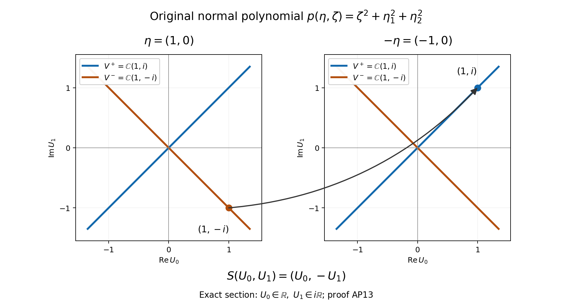
The figure shows the exact section in AP13 for the original scalar Laplacian and the two indicated covectors. The arrow identifies the original point with its reflected point ; it does not depict a trajectory. The full complex jet spaces and their exact projection remain given by AP13.
The principal identity is not an identity for every lower-order normal equation. A concrete full differential polynomial is Here , so the full frozen positive and negative solutions are and . Their jets prove the displayed full projection directly, with the original convention and all lower-order terms retained. Its principal polynomial is the elliptic , which satisfies AP6. For the full family, , whereas when . Positivity of both square roots then gives . This is a counterexample for the exact full frozen normal projection; no identification with a particular global choice of the smoothing-corrected Green operator is needed or claimed. AP6 concerns the original principal weighted projection, and the full retains the distinct Green and smoothing arguments of Sections7–11.
10. Why the full defect has a smooth kernel
We now prove the stronger operator assertion Vanishing of the leading symbol alone would give only one order of improvement and is insufficient.
First, maps boundary distributions continuously to and has a smooth kernel on . In fact (CD14) differentiates the smooth kernel of in its input variable a finite number of times and restricts that variable to . Its output derivatives of every order remain smooth and bounded on the compact working set.
Second, zero extension of , initially for smooth , has a continuous distributional extension Here and below an output cutoff equal to one near makes the displayed compact-support convention literal. Define this extension by duality: The right side uses boundary derivatives through normal order . Their values are unambiguous. To check this explicitly, has order , so it takes the localized section into . After any number of tangential derivatives the result is still locally : commute such derivatives through ; each commutator is again of order , and tangential differentiation commutes with zero extension. Iterating, with compact cutoffs, proves the assertion to every tangential order. Fourier Cauchy–Schwarz in the tangential variables and the one-dimensional inequality now give common two-sided values of every required normal derivative. The one-dimensional inequality follows directly by integrating against the weight, since its squared reciprocal tail is . In addition, the adjoint transmission proved in Section 5 gives smooth one-sided restrictions, continuously in the smooth seminorms of .
It follows that the transpose boundary expression applied to is a smooth section of the dual Cauchy bundle, continuously in . Pairing with any boundary distribution defines (CD29) and proves its continuity. For smooth , approximate by functions vanishing near , using cutoffs depending only on . Their zero extensions converge in , with every tangential derivative. The preceding argument makes the relevant boundary derivatives of their images under converge. Ordinary distributional duality away from gives (CD29) for each approximation; passing to the limit gives , proving (CD28). No multiplication of an arbitrary distribution by the discontinuous indicator of was used.
The map has a smooth kernel on . This can be proved directly, without interpreting weak continuity as smoothing: insert each smooth input-variable kernel section of into (CD29). It depends smoothly on the output point with all derivatives; the continuous adjoint-transmission map in (CD29) makes its resulting boundary section jointly smooth. Differentiating this section proves the smooth-kernel assertion. Similarly has a smooth kernel: for each boundary input point its -kernel section is smooth on , smoothly depending on that point, and the smooth transmission map preserves this dependence.
Apply (CD19) to , for smooth . By (CD16) and (CD17) it gives Thus , a difference of the two smooth kernels just proved. Smooth boundary functions are distributionally dense by chartwise convolution and partition, and every operator in the identity is continuous on distributions. Therefore the identity and (CD27) hold on all boundary distributions. The argument proves smoothing at every order, with the actual remainder kernels from (CD10), and never assumes (CD27) in order to define .
11. The positive trace of an interior particular solution
The particular-solution trace obeys the useful gain The factor here is , with the inward convention of (CD12).
For smooth , let , smooth by transmission. Then , while . Insert these into (CD19) and cancel . The exact remaining identity is Each term is continuously smooth for . For the first, zero extension is bounded in , the local order theorem gives , restriction and then zero extension are bounded in , and is smoothing. For the second, is continuously smooth on a neighborhood of , so its restriction, followed by the smooth transmission map of and the boundary trace, is smooth. The bounds apply to every output derivative. Also is continuous by the same estimate and (CD3), so the left side of (CD32) is already well-defined for inputs by (CD21). Smooth approximation in extends the equality and proves (CD31). This derivation keeps both parametrix remainders and does not require an invertible extension.
12. What the boundary reduction actually says
For a smooth solution of , set . With from (CD6), the exact boundary identities are The term is smoothing in the interior unknown, whereas is fixed by the forcing. Thus the first equation determines the nonpositive-mode component of the Cauchy vector, modulo a smoothing term. The trace of the forcing has smooth by Section 11; is also smooth, since pseudodifferential operators preserve smooth sections. In particular is smoothing in , quantitatively for . This explains the compatibility among the apparent Cauchy equations: at the symbol level is prescribed and the remaining data lie in .
For every , (CD33) has the spaces The particular trace has this regularity when with , by (CD19): both and lie in , and is smooth. Independently on arbitrary requires the appropriate truncated-operator mapping theorem for that scale; it is not deduced from the unrestricted zero extension , which can fail. The exact statement needed above has already been proved. The adjoining boundary Fredholm unit establishes the further mapping and projected inverse statements.
Conversely, simply choosing satisfying a version of (CD33) with the smoothing term omitted is not an exact existence proof for the original differential problem. The remainders (CD17)–(CD19) must be corrected or included in a Fredholm argument. This lesson supplies the full Cauchy construction and the compatible weighted symbol, and leaves that general solvability obligation to its separate proof.
13. Four calculations that expose different constraints
A first-order system with a changing stable rank. On a two-dimensional collar consider , where on , , . Its principal determinant is , nonzero for every real . The normal solution is For every initial vector is stable, whereas for no nonzero initial vector is stable. Thus on the positive ray and on the negative ray. The polynomial factor retains the generalized modes. At a given boundary point a differential boundary target bundle has a single fixed rank, so it cannot be bijective from both a rank-two and a rank-zero stable space. This is a concrete failure of the local complementing test for every such choice of target rank, despite interior ellipticity. It does not assert failure of all possible nonlocal spectral boundary constructions.
A fourth-order datum projected onto two decaying rates. Freeze , , and prescribe . The positive modes are and . Their projected combination is To verify the coefficients, decompose in the four Cauchy vectors associated with . Vanishing of the first and third normal jets makes the coefficients of the positive and corresponding negative exponentials equal in the direct-sum decomposition. The zeroth jet gives opposite coefficients for the two rates. The second jet then gives . Applying yields exactly (CD36). The negative contribution in the direct-sum decomposition is subtracted to obtain the actual in (CD25). This computation exhibits the distinct powers in one column of the weighted projection.
A coefficient jet that survives in the jump. Put near . Formula (CD14) gives Indeed , as is verified by pairing with a test function. Evaluating at zero before multiplying would delete the term. That term is lower in the tangential order but indispensable in the exact Green identity and the full projection defect proof.
An idempotent leading symbol is not enough. On the circle let , defined by its Fourier multipliers, and let . The classical order-zero matrix has leading symbol , but Its first diagonal Fourier multiplier is , which does not decrease faster than every inverse power. A smooth kernel on the compact circle would have such rapid Fourier decay by integration by parts in both variables. Hence (CD38) is not smoothing. This is a generic pseudodifferential matrix, not the operator built from (CD16); it shows exactly what the Green identity contributes beyond the residue calculation.
14. Exercises with complete solutions
1. Retain noncommuting coefficients. For constant matrices , with invertible, take . Write the jump distribution and the four leading projection entries, leaving the contour unevaluated.
Solution. The jump is . Formula (CD22) gives the contour integral of the block matrix divided by . Each block is an ordered product. In particular cannot in general be replaced by : multiplying their difference on the left and right by gives the commutator , which can be nonzero. For a tangential principal polynomial has degree zero, degree one and degree two, so the entries after normal integration have degrees , respectively.
2. Check the jet rescaling. Define . Show how is recovered from , and explain why this does not change its rank.
Solution. The -entry of is , equal to by (CD22). Thus the two projections are conjugate by an invertible matrix. Their images and kernels have the same dimensions. The unweighted Euclidean norm of their entries can grow with ; that growth is absorbed by the Sobolev weights in (CD2), rather than contradicting projection rank invariance.
3. Locate the trace threshold. Explain why the proof of (CD3) cannot be continued to , and construct bounded functions whose -th normal traces grow.
Solution. The reciprocal-weight integral has tail . Take a fixed smooth tangential Fourier factor supported where , and set , where is a smooth cutoff supported in , equal to one on , with uniformly scaled endpoints. The squared norm is bounded by a constant times , hence uniformly bounded. Its -th trace has tangential Fourier transform a constant multiple of , up to a bounded relative error tending to zero. Its norm therefore grows. Each is smooth by its compact smooth Fourier support. This disproves a bounded trace into the predicted endpoint target; it does not contradict traces on a solution subspace with additional elliptic information.
4. High tangential order is permitted. For an order-two elliptic equation take the reduced boundary operator . State its target on , and compare it with .
Solution. The total order is eight and the normal order is one. The trace is in , so seven tangential derivatives give . This is the target in (CD7). The expression is not an ordinary trace for a general section. Normal division uses the equation to replace it by a reduced operator and a boundary differential expression in the forcing. The latter expression is meaningful for smooth forcing, but it is not automatically defined for arbitrary forcing.
5. Separate the two halves of complementing. For the frozen polynomial , , measure both and with target . Is the resulting boundary map complementing?
Solution. Every stable solution is , and its two measurements are . This map is injective, but its range is the one-dimensional line with second coordinate times the first. It is not surjective onto , so it is not complementing. With only the first measurement and target it is bijective. This frozen calculation is a test of principal boundary data; a global solvability theorem still requires its analytic argument.
6. Determine the negative-side sign. If is the Cauchy vector of a negative stable solution , what are the two functions obtained from (CD23)?
Solution. Equation (CD26) gives . Hence , so ODE uniqueness gives . The jump equation then reads , and uniqueness gives . The minus sign is forced by the convention “positive trace minus negative trace” in (CD25). Replacing it by would reverse the source term in (CD24).
7. Perturb the parametrix by a smooth kernel. Let , where has a properly supported smooth kernel. Show explicitly that the corresponding differs from by a smooth kernel, while an exact identity need not hold.
Solution. The difference is . In a local expression (CD14), integration against the derivative of differentiates the input-variable kernel of , including the coefficient factors, and restricts it to . Tangential derivatives from do the same in the tangential input variables. The final takes finitely many output normal derivatives and restricts the output to . Thus all resulting entries are smooth on . They need not vanish: choosing a separated kernel with a nonzero relevant input boundary jet and a nonzero output boundary jet generally gives a nonzero finite-rank difference. The principal projection is unchanged, but the full approximate projection has changed.
8. Recover every jump from the top coefficient. Suppose a piecewise normal ODE solution has singular forcing equal to (CD24). Prove that matching only the highest derivative of and the invertibility of starts a complete recovery of all jumps.
Solution. At derivative order , the coefficient of the difference between the actual forcing and (CD24), multiplied by , is . For the sum is empty, and invertible gives . If the equalities hold for , the sum vanishes and the same invertibility gives . Induction reaches . No root simplicity is used, and no inverse is commuted through a coefficient. This triangular mechanism is the algebraic content behind the full distributional jump.
15. The exact receiving boundary distribution
Every original normal coefficient jet in the boundary distribution is unchanged. This is the whole original (CD14), with its triangular index range, its factor , and coefficients acting after multiplication by the normal delta derivative. A test supported away from has every normal derivative zero along , so each pairing in (CJ19) vanishes; the support remains on the compact original boundary. Coefficient multiplication against a delta derivative uses the actual normal jets up to that derivative order. Equations (CJ6)–(CJ7) preserve all of them, so the extension changes no term of this boundary operator or of the exact jump identity (CD15).
Choose a relatively compact open neighborhood of inside the displayed ambient domain by retaining the negative collar only through . Its closure lies inside that domain since and are compact. The existing properly supported bundle calculus therefore applies there to this full original differential extension and supplies (CD10) with both original error sides. This completes the globalization, bundle transport, smooth supported coefficient extension and ellipticity persistence used in Section 4. It asserts neither an invertible closed double nor an exact solution obtained by dropping a smoothing remainder.
Further questions and references
Lashi Bandara, Magnus Goffeng and Hemanth Saratchandran, Realisations of elliptic operators on compact manifolds with boundary, arXiv:2104.01919v2, Sections 3.1–3.2 and 9, supply a freely accessible higher-order treatment of the graded jets, approximate and exact Calderón projections, and the mixed regularity of maximal-domain traces. Their Section 3.1 states the approximate projection theorem by citation; Sections 5–11 above give the complete receiving proof with every layer order and both smoothing remainders.
The separate editorial note Calderón projections: trace phases, residues and boundary norms, BC1–BC28, proves the exact change between their ordinary derivative traces and our original D traces. It corrects the source’s printed trace phase, residue phase and row-versus-column degree using complete scalar counterexamples and the unchanged original matrix products. It also records the exact antipodal rank qualification and proves a Fourier model of their off-diagonal compactness condition. These corrections concern the identified source version; the construction and mathematical formulas above are retained. The source’s additional global Hardy-space and sectorial-projector statements require their respective proofs and are not deduced from an approximate projection alone.
Three next questions distinguish what the construction already gives from what requires further work. First, a boundary matrix bijective on suggests an inverse on that projected symbol bundle. Constructing a full operator inverse modulo compact remainders, with all Sobolev orders and smooth cokernel descriptions, is the next Fredholm problem. Second, an approximate projection can sometimes be corrected by a smoothing operator to an exact projection with an appropriate global Cauchy range. Its finite-dimensional correction and dependence on the extension must be proved, rather than inferred from (CD27). Third, parameter-dependent stable bundles can carry topological obstructions to local differential boundary conditions, as the first worked model already detects at the rank level. More refined obstructions require global bundle and index arguments.