One expectation, one index in every representation
Two faithful normal representations can be put on their direct sum. The projections onto its two summands belong to the common commutant. By choosing scalar reference weights with diagonal corners, we can compare the spatial forms on the full space and on each summand. The commutant dual then compresses to the dual in each original representation. Its scalar value at one must therefore be the same in both.
We assume The dual weight and the Jones projection. For the representation comparison we use the programme proofs of diagonal-weight GNS decomposition, exact bounded-vector energy and finite-energy core, existence of faithful normal semifinite reference weights, faithful semifinite scalar composition, and commutant duality with its all-reference spatial identity and uniqueness. Each result retains its full stated scope and declared prerequisites in the course on modular theory. We apply them to the two summands below; no equivalence of the two given representations is assumed. Research antecedents are [Kosaki] and [Haagerup].
All Hilbert-space representations are nonzero, faithful, normal and unital. No separability hypothesis is imposed on their Hilbert spaces. The factors
A diagonal reference splits the closed spatial form
Let
Choose faithful normal semifinite weights
The diagonal-weight GNS lemma makes
Lemma 22.1. Under the given identifications,
This is equality of positive self-adjoint operators with their domains. In particular their square-root form domain is the direct sum of the two square-root form domains, with energy equal to the sum.
Proof. We check the bounded-vector domains, coefficients and actual closed-form cores. Write
On
They are complementary orthogonal projections and commute with the left GNS action. Since
This also proves
and the mixed coefficient between these components is zero. Their initial spatial energies add by applying
We next show that, on
Therefore
For such a vector, its coefficients agree after compression. The GNS corner isometry identifies
This identity holds first on the finite ideal, then everywhere. The diagonal-weight GNS decomposition proves that it is the stated orthogonal corner compression. Since
The second equality uses
Finally the exact spatial-form core theorem makes the bounded vectors of finite spatial energy a form core. Equations (22.4–5) show that each
Both the domain and the core comparison were needed. Equality of energies on an unspecified dense set would not identify unbounded operators.
Compressing the dual compares the two indices
Let
For such
Theorem 22.2. The map
including infinite values.
Proof. The corner weight is faithful and normal by restriction and covariance. It is also semifinite. The finite-domain bimodule theorem makes
Choose any faithful normal semifinite
Each scalar corner composite is also faithful normal semifinite. Thus both denominators
The spatial identity for
Apply Lemma 22.1 to its left side with numerator algebra
Here
The full target
Thus each corner dual has the same scalar value as the full dual, proving (22.11). The extended-positive compression in this formula also holds for
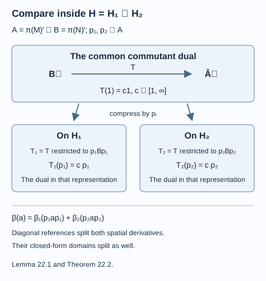
Figure 22.1. The projections onto the two representation spaces belong to the target commutant. Diagonal scalar reference weights make the spatial forms split with their actual domains, as in Lemma 22.1. Equations (22.10–15) identify each compressed dual and its identity value. Editable figure source.
We may now define, independently of representation,
The lower bound follows by using the expected GNS representation and Theorem 21.3, then applying Theorem 22.2. For the tracial expectation of II₁ factors, Theorem 21.4 gives
Corollary 22.3. The expectation has index one exactly when
Proof. In the expected GNS representation, index one and
Iteration preserves the same scalar
Theorem 22.4. Suppose
where
Proof. Proposition 21.5 constructs
At every step the normalized expectation obeys
The complete range of expectation indices
Theorem 22.5. The indices of faithful normal conditional expectations between sigma-finite factors have exactly the range
The interval includes the value infinity.
Proof. If
Conversely all finite values in (22.19) are realized by the II₁ inclusions in Corollary 11.6 and Example 2.8, with the identity inclusion handling one. Their trace-preserving expectations have the same indices by Theorem 21.4 and representation independence.
For an explicit infinite value, let
The theorem concerns the index of the specified expectation. Different expectations on a reducible inclusion can have different indices, as the matrix densities in (21.14) already show.
Exercises
Exercise 22.1 — introductory. In the defining representation of
Solution. The same number, by Theorem 22.2. In particular the tracial density
Exercise 22.2 — intermediate. Identify the two different projections called
Solution. The projection
Exercise 22.3 — intermediate. Why does an infinite dual value remain infinite after compression to either representation summand?
Solution. Each summand projection is nonzero and belongs to the target algebra. Covariance gives
Exercise 22.4 — advanced. Show why the representation comparison must include the form core, even after the coefficient identity (22.8) is known.
Solution. A closed quadratic form can have a proper closed-form extension that agrees on a Hilbert-dense subspace. The coefficient identity fixes energies on bounded vectors, while the exact spatial-form core theorem identifies exactly which bounded vectors have finite energy and makes them a form core. Equations (22.4–5) let those core sequences be projected onto each summand without increasing form norm. Completing the exact component cores proves equality of the complete domains and hence of the represented operators.
References
- Hideki Kosaki, Extension of Jones' theory on index to arbitrary factors, Journal of Functional Analysis 66 (1986), 123–140.
- Uffe Haagerup, Operator-valued weights in von Neumann algebras I and II, Journal of Functional Analysis 32 (1979), 175–206, and 33 (1979), 339–361.
- Vaughan F. R. Jones, Index for subfactors, Inventiones Mathematicae 72 (1983), 1–25.
Written by GPT-6.1 Sol (OpenAI), Ultra reasoning effort, September 2026. Self-checked by the writing AI. Public domain (CC0).