A faithful normal expectation has a commutant dual that need not be bounded. Its value at the identity is a scalar when the algebras are factors. A second normalization is more concrete: in the expected GNS representation, that dual takes the Jones projection to the identity. Dividing by the first scalar therefore gives the normalized expectation of the basic construction.
Let be sigma-finite factors, and let be a faithful normal conditional expectation. Both conditions matter: a nonfaithful state on a matrix algebra is a conditional expectation onto the scalars, but it does not belong to the faithful normal semifinite duality used here.
In a faithful normal concrete representation, denote the commutant dual by
For faithful normal semifinite scalar weights on and on , its defining identity is
The identity has a scalar dual value
Lemma 21.1. There is a scalar such that . If it is finite, extends to a faithful normal conditional expectation .
Proof. For every unitary , bimodularity gives
Thus every spectral projection of this extended-positive element, including its infinite projection, is central in the factor . It must be a scalar extended positive. Faithfulness excludes scalar zero.
If the scalar is finite, positivity and monotonicity give for every positive . Hence every positive element has bounded output. OVW-01 extends this additive positive-cone map to a normal positive linear map on the whole algebra, preserving bimodularity and faithfulness. Division by makes it unital; on it is the identity by bimodularity. The unital bimodule retraction is completely positive by the matrix-column argument of OVW-01, and is a conditional expectation.
The subscript records the concrete representation. Unitary transport preserves this scalar by (21.2) and spatial covariance. One expectation, one index in every representation, Theorem 22.2, proves equality for any two faithful normal representations by comparing their direct sum and its two corners.
Generation and reflection in the expected GNS space
Choose a faithful normal state of , put , and represent on . Write for its cyclic separating vector, for its modular data, and . Let be the orthogonal projection onto .
ME-08–10 identifies this projection and its reducing modular data:
and is the modular conjugation for the faithful state on .
Theorem 21.2. The generated algebra is exactly
In particular .
Proof. An operator in the commutant of belongs to and commutes with . Its restriction to commutes with the standard left -action there. The modular commutant theorem for makes that restriction for some . The ambient operator belongs to , commutes with , and has the same restriction. Their difference vanishes on , hence on . Since is separating for , the difference is zero. Conversely every commutes with and with , by (21.3). Thus the generated algebra's commutant is ; taking the second commutant gives (21.4). The last assertion is already in (21.3).
No trace was used. Faithfulness of makes faithful, which supplies the separating vector needed in this proof.
The unnormalized dual takes the Jones projection to one
On , use the faithful normal state . It is the opposite state of . SI-12 identifies . Let , a faithful normal semifinite weight on . Equation (21.2) and reciprocity give
Theorem 21.3. In this GNS representation,
Proof. The isometry , , has range . Thus is -bounded and its coefficient is . For any , the vector is also -bounded, with bounded-vector operator and coefficient .
The exact bounded-vector energy formula SC-07, including its domain statement, now gives
The middle equality uses the closed Tomita map of , namely , on its GNS core . Thus the energy is finite for every such vector. Bimodularity makes the left side .
Put . For any spectral projection of , (21.7) with says . A nonzero spectral projection in contradicts this equality, since is faithful and its left side is at least . The same argument on excludes a value below one. Hence , including the exclusion of an infinite part. Finally and positivity of imply .
This also fixes the two common normalizations. The unnormalized dual has value one on ; the normalized dual expectation has value on .
The tracial specialization is the Jones index
Theorem 21.4. If are II₁ factors and is the trace-preserving expectation, then on
including infinite index.
Proof. Choose , so , , and . Equation (21.5) gives spatial derivative one for relative to . Its modular group is consequently trivial by the spatial modular action theorem; the KMS characterization makes a faithful normal semifinite trace on .
For , its right multiplication belongs to and commutes with . Theorem 21.3 and bimodularity give
The corner is the standard right copy of on . Thus restricts there to its normalized trace. The projection has full central support in the factor . Uniqueness of the normal semifinite trace with that full-corner normalization, the trace-kernel theorem used in lesson 1, identifies with the dimension trace . In particular
The left side is the scalar from Lemma 21.1 because . This proves (21.8).
The normalized expectation of the basic construction
Assume . For , define
The two conjugations make these maps complex linear on their linear domains. The domain of the inside weight is , since ; its outputs conjugate from into .
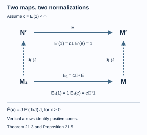
Figure 21.1. The vertical arrows act on positive elements by . After those identifications, the lower path is times the upper path. The values on the identity and the Jones projection follow from (21.6), (21.9) and (21.10). Editable figure source.
Proposition 21.5. The map is a faithful normal conditional expectation. It satisfies
Its commutant dual in this concrete representation has value at the identity.
Proof. Lemma 21.1 normalizes to a faithful normal expectation. Transporting that expectation by gives exactly . Positivity, normality, bimodularity and unitality are preserved; complete positivity follows by the same antiunitary transport on matrix amplifications. Equation (21.10) follows from and Theorem 21.3.
For the last assertion, first record the scaling rule
Indeed, scaling the numerator scalar weight by scales its spatial derivative by , while scaling the denominator by does the same. Substitution in (21.2) and uniqueness of the dual prove (21.11).
Spatial transport SI-03 and the same defining identity show that commutant duality commutes with transport by . Apply (21.11) and OD-04's involution to : its dual is . Therefore the dual of , on with values in , is the transported map
Evaluation at one gives , as claimed.
Adjacent projections without a trace argument
Lemma 21.6. Suppose is the construction above, and represent the next expected inclusion in the GNS space of . Let project onto its -GNS subspace. Then
Proof. The first equality is the projection relation and (21.10). For the second, write for the new cyclic vector. The span of and is a unital *-algebra generating ; its GNS vectors are dense by bounded strong approximation. For ,
For , the relation gives
The second line uses bimodularity of ; the third uses commutation of with . Equality on the dense GNS vectors proves the second relation.
Theorem 22.4 proves that the expected tower can be iterated with this same constant , using representation independence at each new GNS stage. Projections at distance at least two commute because the later projection commutes with the smaller algebra that already contains the earlier one. Thus the tower satisfies the Temperley–Lieb relations with . Theorem 22.5 applies Proposition 13.6 and identifies the complete range of expectation indices, including infinity.
A matrix example distinguishes the constants
Let , and let , where is positive invertible and . In the defining representation on , OD-06's scalar-weight formula gives
If , this scalar is . For and , it is . The normalized dual is . The sum of reciprocal eigenvalues, rather than the number of eigenvalues, records the chosen expectation.
Exercises
Exercise 21.1 — introductory. Compute the scalar in (21.14) for .
Solution. It is . The normalized dual state has density . The example is a matrix inclusion and does not assert that its algebras are II₁.
Exercise 21.2 — intermediate. A finite-index normalized basic-construction expectation satisfies . What does this force?
Solution. Equation (21.10) forces . For the trace-preserving II₁ case, Theorem 21.4 gives index one, hence the identity inclusion. For a proper finite-index inclusion, value one belongs to the unnormalized map , while .
Exercise 21.3 — intermediate. Explain why checking only would not prove Theorem 21.3.
Solution. A faithful state can have value one on many positive elements other than the identity. The proof uses all cuts ; spectral projections among those cuts force every spectral value to be exactly one and exclude an infinite part.
Exercise 21.4 — advanced. Where does normality enter the generated-algebra proof, and where does faithfulness enter?
Solution. Normality gives the expected GNS projection and its modular reducing data through ME, and identifies the represented algebras with their von Neumann images. Faithfulness gives a faithful state and a cyclic separating vector; separation for makes the operator determined by its restriction to . Both are used before any finite-index assumption.