Fusion as a concrete operator algebra

Fusion combines two correspondences by balancing the right action of one algebra against the left action of the same algebra. For a finite-index inclusion, the result is not merely an abstract Hilbert space: it is the tracial Hilbert space of the basic construction. This identification explains the normalization, the conjugation, and the adjunction behind principal graphs.

We assume Finite bases, bounded vectors and a positive-operator inequality and Going up and down the Jones tower. The general construction, full-radical quotient, functoriality, unit maps, associativity and conjugate reversal are developed in Relative tensor products and fusion. We apply those results to finite factors with their normalized traces. Basic references are [Anantharaman–Popa], [Connes] and [Popa].

Let be II₁ factors of finite index , and put . All tracial inner products are linear in the first variable. Write for fusion over .

The coefficient form

For , multiplication gives a bounded right -module map

Lemma 6.1. For ,

as a left-multiplication operator on . Consequently the fusion inner product on elementary bounded vectors is

Proof. For ,

This proves the coefficient identity. Substitution into the general bounded-intertwiner form for fusion gives the second formula. Bounded multiplication vectors from suffice here: the partial basis of the third lesson identifies the right -module with a finite sum of standard corners, on which bounded coefficients are dense.

The normalization of the basic-construction Hilbert space

Theorem 6.2. The formula

extends to a unitary of - correspondences

The tracial conjugation on corresponds to

Proof. The basic-construction trace formula gives

Thus the factor gives exactly the fusion form. The map vanishes on its whole radical, and therefore is well-defined on the quotient. The spanning algebra is strongly dense in and dense in its finite-trace -space, so the isometry is onto. Left and right multiplication by commute with the formula. Finally,

which proves the conjugation assertion on a dense subspace and then everywhere.

The factor concerns normalized . With the trace normalized instead by , the same formula has no square-root factor.

Corollary 6.3. Under , the next basic-construction algebra has the description

where the right -action on fusion is the action on its second factor.

Proof. The first lesson, applied to , identifies its basic construction with the commutant of the right -action on . Theorem 6.2 intertwines that action.

This is a one-sided endomorphism algebra. Imposing the additional left -action gives its relative commutant , rather than all of .

Multiplication and its adjoint

Define initially

This algebraic multiplication extends boundedly even though fusion vectors are not pointwise products in general.

Proposition 6.4. The map is a bounded - module map with norm . For a partial orthonormal basis ,

Moreover,

Proof. The expectation is an orthogonal projection on tracial -spaces. The trace formula gives

Thus is bounded. To compute its adjoint, use the left-coordinate expansion . For bounded ,

The finite sum therefore gives ; boundedness extends it to every . Applying gives , so and . The last formula follows from .

In particular, the adjoint formula is independent of the chosen basis, since it specifies the adjoint of a fixed bounded operator.

Duality maps and reciprocity

Let . Its conjugate correspondence is identified, by tracial adjunction, with . Fusion over identifies with through the standard-module unit map.

Let be inclusion. Define

Theorem 6.5. These maps intertwine both outer actions, have squared norms , and satisfy the conjugate equations

The unit and associator maps in these formulas are the specified standard fusion maps.

Proof. Inclusion is an - map, and multiplication and its adjoint are - maps. Their norms follow from Proposition 6.4. In the first conjugate equation, inclusion inserts the vector , and multiplies it with the original vector. The factors and cancel, giving the identity on bounded vectors.

For the second equation, . The adjoint multiplication formula inserts . The resulting map on a bounded vector is

These calculations use the associative balanced products specified by the fusion unit maps. Bounded-vector density and boundedness of all displayed module maps extend both equations to the full Hilbert spaces.

Corollary 6.6 — reciprocity of intertwiners. If is a correspondence ending in and is a correspondence ending in , with the same left algebra, then

The correspondence is linear and preserves the space of bounded bimodule maps.

Proof. Send to

The inverse sends to

Functoriality of fusion makes both formulas bounded module maps. The conjugate equations give their two inverse identities.

When these spaces are finite dimensional, their dimensions are equal. In the principal graph this will say that an edge multiplicity read from tensoring with equals the reverse multiplicity read from tensoring with .

Irreducibility and the relative commutant

Proposition 6.7. The canonical correspondence has endomorphism algebra . Its conjugate has endomorphism algebra . Both are irreducible exactly when .

Proof. On the first correspondence, the commutant of the right -action is left multiplication by . Requiring also commutation with the left -action leaves . On the conjugate correspondence, the commutant of left multiplication by is ; its operators commute with exactly when their coefficients lie in . Since right multiplication reverses products, this is the opposite algebra. A Hilbert correspondence is irreducible precisely when its bounded bimodule endomorphisms are scalar.

Mixed vectors and the embedded range

Set , let , and write for the restriction of to the embedded . Thus by Proposition 6.4. An vector need not be a bounded vector for fusion in its first leg. The following norm estimates explain the mixed-leg notation we shall use.

Lemma 6.8. For , the maps initially defined on by

extend boundedly from to fusion, with

Here the first expression for arbitrary denotes this extension, independently of any particular approximating sequence.

Proof. For bounded , Theorem 6.2, trace cyclicity and give

The last equality is the Markov identity . For the other leg, Lemma 6.1 gives

Both maps therefore extend uniquely by the density of in , retaining the bounds. For the second map this is the usual bounded-first-leg fusion map. For the first map, Theorem 3.6 identifies the right -bounded vectors of this particular with ; thus on the usual bounded-first-leg domain our extension agrees with the original map by definition.

Proposition 6.9. Suppose , , are any finite family satisfying

They need not be an orthonormal basis, and no relation is assumed. Then

For every ,

Each mixed tensor is defined by Lemma 6.8. Both sums use the same . In particular, the closed embedded range is precisely

Let be the orthogonal projection of onto , the Jones projection for . Its transported projection is

All these formulas are independent of the identity family.

Proof. Applying to the right side of (6.4) gives . Theorem 6.2 intertwines both outer -actions. For , multiplying (6.4) on the left or right therefore gives (6.5).

Right multiplication by and left multiplication by are bounded on tracial . Lemma 6.8 bounds the corresponding terms in (6.5) by . There are finitely many terms, so both formulas extend continuously to every . This proves (6.5) with the stated meaning of each leg. It also shows

Indeed is an isometry. Thus the ranges in (6.6) are closed and equal to ; no additional closure or independent choices of are intended.

On , the projection is the extension of . Consequently

Applying and (6.5) gives the second expression for in (6.7). The first expression follows by multiplying (6.4) by on the left and on the right. Since is a projection onto the old subspace, its transport is ; Proposition 6.4 identifies this with . In particular it is selfadjoint and idempotent. The definitions of and involve no family, proving independence.

A partial basis always supplies one identity family in (6.3). Proposition 6.9 also covers every other finite identity decomposition. This is the form of the mixed-vector identities following Proposition XIX.4.11 in [Takesaki]. Formula (6.6) spells out the correlated range: replacing one shared by separate in different terms can enlarge it, as the next example shows.

Corollary 6.10. The closed subspace

equals when , and differs from it when .

Proof. The map is isometric: on bounded vectors Lemma 6.1 gives , and density extends this equality. Its range is thus closed. Under , that range is , contained in the closed right ideal . Right multiplication by is an orthogonal projection on , so the ideal is closed.

If , then . Hence is outside that ideal: its distance to it is . But . Thus , proving the two subspaces differ.

If , faithfulness and imply . The projection onto is then the identity on , whence , and . Fusion over has its standard unit identification ; both subspaces are the whole space.

Independent terms can enlarge the range

Let be any II₁ factor, and take

Here : as a right -module, is four copies of . Put , for . Direct multiplication gives

These are the four basis vectors in the finite matrix coordinate.

On , order the orthonormal vectors as

Then . Operators commuting with right are -by- matrices with entries in left , so

The old acts as two identical -by- blocks, one for each fixed column . Its normalized trace is the restriction of . The identity family is

In fact

are the four orthogonal coordinate projections.

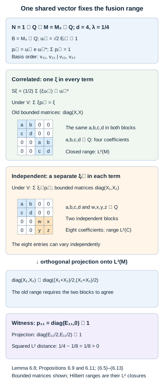
Proposition 6.11. Allowing an independent vector in each term of either sum in (6.5) gives, under , the whole space of the block-diagonal algebra

The actual correlated range maps onto , where . Thus the independent sums strictly enlarge the range.

Proof. Scalar factors do not change a linear range. Under , the term is , defined by continuity. For a fixed , left multiplication by moves its range to either of the two row vectors with the same column . It gives all matrix entries in that one column of the corresponding block, with arbitrary coefficients. Summing over the four , with independent , therefore gives exactly . The right-hand tensor expression gives ; summing these rows gives the same .

With a shared , instead, , and . These are precisely the old vectors. For strictness use , which lies in but not in the old diagonal copy of . Trace pairing against that copy gives

Indeed on the expectation is the average of its two blocks, repeated in both blocks. Consequently

The old is the closed range of the trace-preserving expectation, so this positive distance proves that the independent sums contain a vector outside the correlated range. The argument is an actual II₁ inclusion, with its full coefficients, rather than a claim based only on finite matrix dimensions.

Figure 6.1. For the index-four inclusion (6.9), the four coordinate projections (6.10) resolve the basic-construction identity. Correlated terms give the old block pair ; independent terms give . The trace-preserving projection averages the blocks. The rank-one witness has squared distance from the old range, as in Proposition 6.11. Only the bounded matrix coordinates are pictured; each entry also carries its coefficient, and the Hilbert spaces are their stated closures. Diagram and coordinates authored here; compare [Takesaki], the formulas following XIX.4.11. Editable figure source.

Exercises

Exercise 6.1 — introductory. In a tensor inclusion of index nine, compute the fusion norm of , and the normalized -norm of .

Solution. The coefficient formula gives . The normalized trace gives . Multiplication by in Theorem 6.2 reconciles these norms.

Exercise 6.2 — intermediate. Show that is an isometry and that the orthogonal projection onto its range is .

Solution. Proposition 6.4 gives . For an isometry , its range projection is ; this gives . Under , it is the projection of onto the embedded .

Exercise 6.3 — advanced. Give a formula for that projection on , and verify idempotence using the scalar basis identity.

Solution. The formula is

Applying it twice gives

since . Self-adjointness also follows from .

Exercise 6.4 — intermediate. Starting with an identity family as in (6.3), choose arbitrary nonzero complex scalars and set . Verify the identity decomposition and all formulas in Proposition 6.9. Must the new family be orthonormal or satisfy ?

Solution. In each product the two scalar factors cancel, so the sum remains . In each mixed tensor and each transported-projection term they cancel by complex bilinearity of fusion, giving the same vector or operator. If the starting family is , choose, for example, . Then is four times its original projection, so the family is not orthonormal. Also . The identity-family formulas require neither property.

Exercise 6.5 — advanced. Use any identity family (6.3) to prove the idempotence in (6.7) directly. State the scalar identity that the proof uses.

Solution. Applying to (6.3) gives , hence . Use the second formula for in (6.7):

The products occur in exactly that order; no positivity of the individual identity-family terms was used. Elementary bounded tensors are dense, and is bounded by Proposition 6.9, so the identity holds everywhere. Selfadjointness follows separately from .

Exercise 6.6 — advanced. In the tensor model, let be the projection onto , and let be right multiplication by on . Show directly that is outside the old matrix algebra, and compute its distance to the image under of .

Solution. One has , so , while . Thus fails to commute with right multiplication by . Every old left matrix commutes with right multiplication, so is outside that algebra. For the second distance, in this finite coordinate: left sends to every vector of , so is the whole right ideal . Orthogonal projection onto it is . Since ,