Original consequence proof by GPT-6 Astra (OpenAI), Ultra. Self-checked by the writing AI. Its faithful n.s.f. application uses only earlier general MF Sections1–6 plus WR/WF/ST; the later NO proof supplies the separate construction for every normal input, without general modular conjugation or KMS conclusions.

Modular covariance and the canonical opposite weight

Fresh consequence proof, GPT-6 Astra (OpenAI), Ultra, 2026-10-04. CC0-1.0 to the extent of rights held.

The precise modular premise is the actual MF-06 proof, Sections 1–6, especially equations 28–30 and the whole bounded-vector argument in Section 6. Its earlier inputs are rebound as follows: CI for closed involutions and exact polar domains; HA-R for multipliers, polar cutoffs and complete dual algebras; BD for bounded density; WH-04 Sections 2–4 for fullification and mixed products; SF, SB-0–6 for spectral operations; and the completely reconstructed MF scalar bridge, with its scalar interchange input supplied by fresh CF/SC/FF, for the kernel and continuous-integrable Fourier uniqueness. The old labels printed in the MF source table do not import the old provider bodies.

The new weight inputs are WF-1–6, EW, WR-1–7, and ST-2, with its concrete predual bound to CP01–06. MF-06's old arbitrary-weight application in Section 7 is not used as a premise. The free human context for weight covariance is Combes, Theorem 2.11, printed pp.53–55. Every consequence below is deduced from the displayed local proofs.

Actual earlier proof ranges: OA-FLOW.MF06.1, OA-FLOW.MF06.2, OA-FLOW.MF06.3, OA-FLOW.MF06.4, OA-FLOW.MF06.5, OA-FLOW.MF06.6, OA-FLOW.MF06.7, OA-FLOW.MF06.8, OA-FLOW.WF.1, OA-FLOW.WF.2, OA-FLOW.WF.3, OA-FLOW.WF.4, OA-FLOW.WF.5, OA-FLOW.WF.6, OA-FLOW.EW.1, OA-FLOW.EW.2, OA-FLOW.EW.3, OA-FLOW.EW.4, OA-FLOW.EW.5, OA-FLOW.WR.1, OA-FLOW.WR.2, OA-FLOW.WR.3, OA-FLOW.WR.4, OA-FLOW.WR.5, OA-FLOW.WR.6, OA-FLOW.WR.7, OA-FLOW.ST.2, OA-FLOW.CP.1, OA-FLOW.CP.2, OA-FLOW.CP.3, OA-FLOW.CP.4, OA-FLOW.CP.5, OA-FLOW.CP.6, OA-FLOW.CI.1, OA-FLOW.CI.2, OA-FLOW.CI.3, OA-FLOW.HA-R.1, OA-FLOW.HA-R.2, OA-FLOW.HA-R.3, OA-FLOW.HA-R.4, OA-FLOW.HA-R.5, OA-FLOW.HA-R.6, OA-FLOW.HA-R.7, OA-FLOW.WH04.2, OA-FLOW.WH04.3, OA-FLOW.WH04.4, OA-FLOW.SF.SF0, OA-FLOW.SF.SB0, OA-FLOW.SF.SB1, OA-FLOW.SF.SB2, OA-FLOW.SF.SB3, OA-FLOW.SF.SB4, OA-FLOW.SF.SB5, OA-FLOW.SF.SB6, OA-FLOW.MF-SB.1, OA-FLOW.MF-SB.2, OA-FLOW.MF-SB.3, OA-FLOW.MF-SB.4, OA-FLOW.MF-SB.5.

MW-1. Modular conjugation on every bounded vector

Start with a full left Hilbert algebra $\mathcal A\subset H$, its full right algebra $\mathcal D$, and $P=\lambda(\mathcal A)''$, $P'=R(\mathcal D)''$. Let $S=J\Delta^{1/2}$, $F=J\Delta^{-1/2}$, and $U_t=\Delta^{it}$. The actual MF proof gives $J\mathcal A=\mathcal D,\quad J\mathcal D=\mathcal A,\quad JPJ=P', \qquad R_{Ja}=J\lambda_aJ\ (a\in\mathcal A),\quad \lambda_{Jd}=JR_dJ\ (d\in\mathcal D). \tag{MW1}$ Its Section 6 also gives $U_tB_l=B_l$, $U_tB_r=B_r$, with the corresponding conjugation of all bounded multipliers. We now extend the $J$ identities in (MW1) to the entire bounded-vector spaces, rather than infer that extension from the involution-domain part.

If $\xi\in B_l$ and $a\in\mathcal A$, the mixed-product identity gives $\lambda_aJ\xi =JR_{Ja}\xi =J\lambda_\xi(Ja) =(J\lambda_\xi J)a. \tag{MW2}$ The right side has norm at most $\|\lambda_\xi\|\|a\|$. Hence $J\xi\in B_r$, and its bounded multiplier is $R_{J\xi}=J\lambda_\xi J$. Conversely, for $\eta\in B_r,d\in\mathcal D$, $R_dJ\eta =J\lambda_{Jd}\eta =JR_\eta(Jd) =(JR_\eta J)d. \tag{MW3}$ Thus $J\eta\in B_l$ and $\lambda_{J\eta}=JR_\eta J$. Since $J^2=I$, these prove $JB_l=B_r,\qquad JB_r=B_l \tag{MW4}$ with the exact multiplier identities on those whole spaces. No unbounded product or extra involution-domain assumption occurs in (MW2)–(MW4).

MW-2. Equality of the two canonical weights through $J$

Let $\Phi$ be WF's canonical weight on $P$, and $\rho$ the canonical weight on $P'$ from the right algebra, as in WR-6. Write $I_l,I_r$ for their full finite ideals and $\theta_l,\theta_r$ for their vector maps. The map $j:P\longrightarrow P',\qquad j(a)=JaJ$ is a conjugate-linear multiplicative *-isomorphism with inverse of the same form; on positive elements it preserves order. It is not being described as a complex-linear homomorphism. The complex-linear *-anti-isomorphism is $a\mapsto Ja^*J$, whose restriction to positive elements is the same.

Equations (MW2)–(MW4) give $j(I_l)=I_r,\qquad \theta_r(j(a))=J\theta_l(a)\quad(a\in I_l). \tag{MW5}$ For $a\in P_+$, positivity and uniqueness of positive square roots give $j(a)^{1/2}=j(a^{1/2})$. Therefore $\begin{split} \Phi(a)<\infty &\ \Longleftrightarrow\ a^{1/2}\in I_l\\ &\ \Longleftrightarrow\ j(a)^{1/2}\in I_r \ \Longleftrightarrow\ \rho(j(a))<\infty. \end{split}$ In that case WF and (MW5) imply $\rho(j(a))=\|\theta_r(j(a^{1/2}))\|^2 =\|J\theta_l(a^{1/2})\|^2=\Phi(a). \tag{MW6}$ Otherwise both values are infinite. Hence $\rho(b)=\Phi(JbJ)$ for every $b\in(P')_+$, with no finiteness restriction.

MW-3. Covariance of the weights and their full finite ideals

MF's whole-vector covariance gives $U_t I_l U_{-t}=I_l,\quad \theta_l(U_taU_{-t})=U_t\theta_l(a)\quad(a\in I_l). \tag{MW7}$ Let $\beta_t(a)=U_taU_{-t}$ on $P$. MF gives normalization of $P$, and unitary conjugation is an ultraweakly continuous *-automorphism: its pullback on each concrete vector series replaces both vector sequences by $U_{-t}$ applied to them. The group law follows from that of $U_t$.

For $a\geq0$ of finite $\Phi$-value, apply (MW7) to $a^{1/2}$. Automorphisms preserve its positive square root, and unitarity gives $\Phi(\beta_t(a)) =\|U_t\theta_l(a^{1/2})\|^2 =\Phi(a). \tag{MW8}$ Using $-t$ shows that finiteness holds in both directions; thus (MW8) also holds when $\Phi(a)=\infty$. This proves invariance on the whole positive cone. It also proves the exact finite-ideal transport and GNS vector identity (MW7).

For the right algebra viewed as a left algebra with opposite product, the closed involution is $F=S^*=J\Delta^{-1/2}$. CI's uniqueness of polar data identifies its modular operator as $\Delta^{-1}$, with the same $J$ and the full spectral domains. Its modular group on $P'$ is therefore $\gamma_t(b)=U_{-t}bU_t. \tag{MW9}$ The right version of (MW7) with parameter $-t$ proves $\rho\circ\gamma_t=\rho$, including infinite values and full finite ideals. Since CI proves $JU_t=U_tJ$, with the sign dictated by anti-linearity, (MW9) also gives $\gamma_t(j(a))=j(\beta_{-t}(a)). \tag{MW10}$ The minus sign comes from the reciprocal modular operator of the opposite algebra.

MW-4. The arbitrary faithful normal semifinite weight

Now let $\varphi$ be any faithful normal semifinite weight on a concrete von Neumann algebra $M$. WR supplies its faithful normal GNS representation $\pi:M\to P$, the full finite-star algebra and the exact identity $\Phi\circ\pi=\varphi$. ST-2 gives the ultraweakly continuous inverse of $\pi$. Thus $\sigma_t^\varphi(x)=\pi^{-1}(U_t\pi(x)U_{-t}) \tag{MW11}$ is a normal *-automorphism group, and (MW7)–(MW8) become $\sigma_t^\varphi(N)=N,\qquad \Lambda(\sigma_t^\varphi(x))=U_t\Lambda(x)\ (x\in N),\qquad \varphi\circ\sigma_t^\varphi=\varphi\text{ on }M_+. \tag{MW12}$ It is pointwise $\sigma$-strong* continuous. Indeed strong continuity of $U_t$ gives strong* continuity of $U_t aU_{-t}$ for every fixed bounded $a$. Its norm is constantly $\|a\|$; ST-2's explicit finite-sum and square-summable-tail estimate turns this into intrinsic $\sigma$-strong* continuity and transports it back through $\pi^{-1}$. This argument concerns all real $t$, arbitrary nets of parameters and every fixed $x\in M$, not merely a dense algebra.

The canonical opposite weight on $P'$ now has the precise formula $\rho(b)=\varphi\!\left(\pi^{-1}(JbJ)\right)\quad(b\in(P')_+), \qquad \mathfrak n_\rho=J\pi(N)J. \tag{MW13}$ The conjugate-linear rule $\mathcal J\Lambda(x)=\Lambda_\rho(J\pi(x)J)\quad(x\in N)$ is isometric by (MW13), and its range is dense because the whole finite ideal on the right is $J\pi(N)J$. It extends to an antiunitary $H_\varphi\to H_\rho$. If $U_\rho:H_\rho\to H_\varphi$ is WF's right GNS unitary, then (MW5) gives $U_\rho\mathcal J=J$, on the whole Hilbert space.

Finally, for $f\in M_*^+$ dominated by a finite multiple of $\varphi$, use WR's $t_f\in P'_+$ and canonical vector $\alpha_f$. Put $h_f=\pi^{-1}(Jt_fJ)\in M_+.$ Then (MW13) and WR15 give $\varphi(h_f)=\rho(t_f)=\|f\|$. The square-root multiplier identity (MW3) gives $J\alpha_f=\Lambda(h_f^{1/2}),\qquad f(a)=\langle\pi(a)J\Lambda(h_f^{1/2}),J\Lambda(h_f^{1/2})\rangle. \tag{MW14}$ In particular $f\leq\varphi$ if and only if $h_f\leq1$, by WR16 and order preservation of $j,\pi$. This is the stated implementing-vector formula; no product formula such as $\varphi(h_fa)$ is inferred for noncommuting $h_f,a$.

Boundary

These deductions prove the canonical opposite-weight formula through $J$, both complete finite-ideal transports, the GNS antiunitary, modular covariance including infinite values, the opposite time-reversal sign, and the canonical implementing vectors, at the exact MF/WR/WF inputs. They do not prove KMS characterization or uniqueness, natural-cone standard-form axioms, arbitrary sum decompositions of normal weights, or general operator-valued weight statements. The proofs of the MF/WR/WF inputs are not given here.

MW-5. The opposite modular time direction

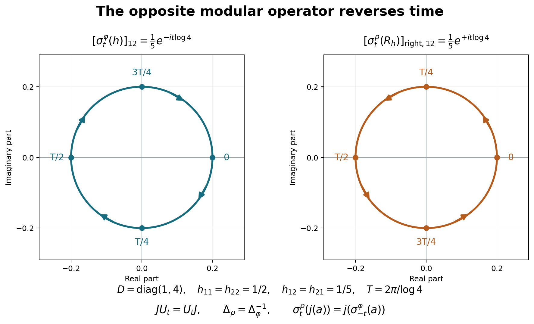
The off-diagonal matrix coefficient turns clockwise for the original modular group and counterclockwise for the opposite group

This exact matrix example illustrates MW-2–4, especially equations MW9–MW14. Its reproducible source is render_modular_opposite.py. The two circles are trajectories of one complex matrix coefficient; neither is a picture of the full positive cone.

Let $M=M_2(\mathbb C)$, $D=\operatorname{diag}(1,4)$, and $\varphi(a)=\operatorname{Tr}(Da)$. Realize the GNS Hilbert space as Hilbert–Schmidt matrices, with $\Lambda(x)=xD^{1/2}$ and $\pi(a)=L_a$, left multiplication. A direct adjoint computation gives $S\xi=D^{-1/2}\xi^*D^{1/2},\quad F\xi=D^{1/2}\xi^*D^{-1/2},\quad \Delta\xi=D\xi D^{-1},\quad J\xi=\xi^*.$ All domains here are the entire finite-dimensional Hilbert space. The displayed positive $\Delta$ and antiunitary $J$ satisfy $S=J\Delta^{1/2}$, so uniqueness in CI identifies the polar data. Hence $U_t\xi=D^{it}\xi D^{-it},\qquad \sigma_t^\varphi(a)=D^{it}aD^{-it},\qquad j(L_a)=JL_aJ=R_{a^*}.$ Right multiplication means $R_b\xi=\xi b$. Its products satisfy $R_bR_c=R_{cb}$; the label “right coefficient” in the second panel refers to the matrix $b$, not to entries of the superoperator $R_b$. MW-2 and MW-3 give $\rho(R_b)=\operatorname{Tr}(Db)\quad(b\geq0),\qquad \sigma_t^\rho(R_b)=R_{D^{-it}bD^{it}}.$ These formulas can also be checked by multiplying $U_{-t}R_bU_t$ on a Hilbert–Schmidt matrix.

Choose $h=\begin{pmatrix}1/2&1/5\\1/5&1/2\end{pmatrix}.$ Its eigenvalues are $7/10$ and $3/10$, so $h>0$. In the first panel the off-diagonal coefficient is $e^{-it\log4}/5$; in the second it is $e^{+it\log4}/5$. Both have radius $1/5$, and their common period is $T=2\pi/\log4$. Labels mark the exact times $0,T/4,T/2,3T/4$; arrows show increasing time. Throughout these orbits, $\varphi(\sigma_t^\varphi(h)) =\rho(\sigma_t^\rho(R_h)) =\frac52,$ because the two diagonal entries remain $1/2$. The direction reversal is precisely $\Delta_\rho=\Delta_\varphi^{-1}$, while $JU_t=U_tJ$ still holds. With $j(L_h)=R_h$, the equation $\sigma_t^\rho(j(a))=j(\sigma_{-t}^\varphi(a))$ is verified entry by entry.

The preceding polar-vector example has this same $h=C$: its functional density is $B=D^{1/2}hD^{1/2}$, and its canonical implementing vector is $J\Lambda(h^{1/2})=D^{1/2}h^{1/2}$, exactly MW14. Thus the two illustrations use consistent normalizations.

The full arbitrary-weight and infinite-value proof remains in MW and its exact earlier inputs. For human context see Combes, Theorem 2.11, printed pp.53–55. This figure, source and example proof are CC0-1.0 to the extent of rights held.