Hilbert modules and fields on the leaf space

Public domain (CC0).

Introduction

A vector bundle over an ordinary space has a module of sections. A foliation has an analogous module over its convolution algebra. Its values are Hilbert spaces associated with holonomy covers, and its inner product is a kernel on the holonomy groupoid. The module norm is an operator norm, so completing the sections can produce elements without a pointwise value. Multiplication by a sufficiently regular kernel restores such values.

This lesson constructs the relation between modules and these fields, proves the norm and endomorphism statements, and explains compact module operators. A compact module operator need not be compact on a single noncompact leaf. This distinction is essential for the analytic index.

We assume C*-algebras, positivity, and Hilbert-space tensor products. The geometric prerequisite is The C*-algebra of a foliation. Square-integrable groupoid representations are developed in Square-integrable representations and random operators. Basic references are [Connes], [Kasparov], [Meyer], and [Landsman]. Inner products in this lesson are conjugate-linear in the first variable and linear in the second.

1. Hilbert C*-modules

A freely accessible reference for this section is [Landsman], Sections 3.2–3.3: module Cauchy–Schwarz, adjointable maps and compact module operators.

Let \(A\) be a C*-algebra. A right Hilbert \(A\)-module \(E\) is a right \(A\)-module with an \(A\)-valued inner product satisfying

with equality in the last expression only for \(\xi=0\), and complete for \(\|\xi\|=\|\langle\xi,\xi\rangle\|^{1/2}\).

Lemma 1.1 (Cauchy–Schwarz).

Proof. Put \(c=\langle\eta,\eta\rangle\), \(b=\langle\xi,\eta\rangle\), and \(a_0=\langle\xi,\xi\rangle\). Work in the unitization when needed. For \(\varepsilon>0\), positivity of

gives

Taking norms and letting \(\varepsilon\downarrow0\) gives the first inequality. The second follows from \(\langle\xi a,\xi a\rangle=a^*a_0a\). The first inequality also proves the triangle inequality and continuity of the inner product, so completion of a pre-Hilbert module is well defined. \(\square\)

A bounded module map is adjointable if a bounded module map \(T^*\) satisfies \(\langle T\xi,\eta\rangle=\langle\xi,T^*\eta\rangle\). Write \(\mathcal L_A(E)\) for these maps. They form a C*-algebra. The adjoint is part of the requirement; bounded module maps need not have one.

For \(\xi,\eta\in E\), define

Its adjoint is \(\theta_{\eta,\xi}\). Cauchy–Schwarz gives \(\|\theta_{\xi,\eta}\|\le\|\xi\|\|\eta\|\). The closed linear span of these maps is \(\mathcal K_A(E)\), the algebra of compact module operators. It is an ideal in \(\mathcal L_A(E)\), because

For later use, \(\|\theta_{\xi,\xi}\|=\|\xi\|^2\). The upper bound was proved above; for the lower bound, with \(a_0=\langle\xi,\xi\rangle\),

Dividing by \(\|\xi\|^2=\|a_0\|\) proves the claim when \(\xi\ne0\).

2. Passing to a Hilbert-space representation

This construction is Rieffel induction; [Landsman], Construction 3.5.3, gives another account with the same inner-product convention.

Let \(\pi:A\to\mathcal L(H)\) be a nondegenerate *-representation. On the algebraic balanced tensor product put

For finite sums this is positive. To verify positivity, the Gram matrix \((\langle\xi_i,\xi_j\rangle)\) is positive in \(M_n(A)\): for a column \((a_i)\), its quadratic expression is \(\langle\sum_i\xi_i a_i,\sum_j\xi_j a_j\rangle\ge0\). Testing after a faithful representation, and approximating arbitrary vectors by columns of represented algebra elements applied to vectors, gives the matrix positivity criterion. Quotient by vectors of zero length and complete. The resulting Hilbert space is \(E\otimes_\pi H\).

Every \(T\in\mathcal L_A(E)\) induces \(T\otimes1\), with adjoint \(T^*\otimes1\) and norm at most \(\|T\|\). One way to check the bound is to apply the same Gram-matrix argument to the positive module operator \(\|T\|^2-T^*T\). Positivity of that operator follows from the C*-identity in \(\mathcal L_A(E)\); it is equivalent to nonnegativity of all its inner-product quadratic forms.

For a family of representations \((\pi_x)\) whose direct sum is faithful,

Indeed the right side is at most the left. In the other direction, a bound \(c\) on every represented \(T\) gives

for every \(x\). Faithfulness of their direct sum reflects positivity, and taking norms yields \(\|T\xi\|\le c\|\xi\|\).

3. Regularized values on the holonomy groupoid

Put \(A=C_r^*(V,F)\), and use the source-fibre representations \(\pi_x\) of the preceding lesson. Choose a positive leafwise density temporarily to write scalar values. Let \(\mathcal C=C_c^{\infty,0}(G,\Omega^{1/2})\), interpreted through chart-supported sections for a non-Hausdorff groupoid.

An element \(a\in A\) need not have a pointwise kernel. We use the dense algebraic left ideal

Every element of this ideal has source-fibre vectors \(f_x\in L^2(G_x)\). For \(f\in\mathcal C\), this is restriction to \(G_x\); for \(a*f\), it is \(\pi_x(a)f_x\).

Lemma 3.1. These vectors are well defined, independent of the expression in \(\mathcal C_2\), and

The set of \(f_x\) for \(f\in\mathcal C\) is dense in \(L^2(G_x)\).

Proof. Restrict a chart kernel to a source fibre. Its compact support and smoothness there give an \(L^2\) vector. For a compact set of base points these vector norms are uniformly bounded, by the chart-volume estimate in the preceding lesson. Hence if \(a_n\to a\) in \(A\), then \(\pi_x(a_n)f_x\to\pi_x(a)f_x\), uniformly in \(x\) on such sets. This constructs the vectors for \(a*f\).

It also makes their dependence on a varying input point continuous along a plaque, with values in \(L^2\) after the local covering identifications: it holds for the chart kernels and passes through the uniform estimate. If a finite expression is zero in \(A\), its represented operator has zero kernel as a distribution in its input variable. Pairing each constructed column with a smooth compactly supported output vector gives a continuous function of the input plaque variable. That function vanishes almost everywhere and therefore everywhere. At the unit input point this says that the constructed column is zero. This proves independence and the displayed rule.

Finally any compactly supported smooth function on \(G_x\) can be partitioned into finitely many lifted plaque patches. Each piece extends to a chart kernel by a transverse bump equal to one at the specified base point. These functions are dense in \(L^2(G_x)\). \(\square\)

This assertion concerns the regularized ideal, not a continuous evaluation map on all of \(A\). For a pair groupoid, a compact operator can have a kernel with no value at a specified input point.

Canonical columns beyond the smooth core

The phrase “restriction makes sense” needs a convention when the kernel is a distribution. Here is one that uses the represented operator itself, rather than a chosen representative of a measurable function. It also describes exactly the compatibility needed if a different column convention is used.

Fix \(x\), a plaque coordinate \(t\) centred at the unit in \(G_x\), and write the temporary leaf density as \(d\nu_x=\rho(t)\,dt\). For \(\varphi\in C_c^\infty(\mathbb R^p)\), put, for sufficiently small \(\varepsilon>0\),

This is an \(L^2\) vector supported near the unit; its integral against \(d\nu_x\) is \(\int\varphi\). We say that \(a\in A\) has a canonical weak column at \(x\) if there is \(a_x\in L^2(G_x)\) such that

The arrow denotes weak Hilbert-space convergence. Let \(\mathcal I\) be the full domain of elements having these columns at every \(x\). No bound on \(\sup_x\|a_x\|_2\) is required. In dimension zero the unit has positive counting mass: use its delta vector, so \(\mathcal I=A\). A scalar column is expressed using the chosen density; intrinsically it also carries the half-density at its source.

Lemma 3.2 (coordinate, density and measurability). Condition (15) is independent of the plaque coordinate. Its columns are unique and measurable in \(x\). Changing the temporary density changes their scalar expressions by the usual two-endpoint half-density rule.

Proof. Uniqueness follows by taking a test of integral one. For coordinate independence we need a uniform estimate for varying tests. Fix a compact test support \(K\). The maps

are continuous linear maps. For each fixed test their values are norm bounded: weak convergence gives this by the Hilbert-space uniform boundedness principle. The complete Fréchet space \(C_K^\infty\) is a countable union of the closed sets \(\{\varphi:\sup_\varepsilon\|S_\varepsilon\varphi\|\le n\}\). Baire's theorem gives an interior point of one of these sets. Subtract two elements in that interior and rescale. There are consequently \(C,m\) such that

The parameter can be restricted to a fixed small interval; its remaining compact interval is bounded directly from (14).

If \(t=F(z)\), \(F(0)=0\), a test normalized in \(z\) becomes in \(t\) a test with rescaled profile

All these profiles have one compact support for small \(\varepsilon\), and converge with every derivative to \(\varphi((DF(0))^{-1}w)|\det DF(0)^{-1}|\). Their integrals equal \(\int\varphi\). Estimate (16) controls the difference from the limiting profile. Thus (15) gives the same column in the other coordinate.

For \(d\nu'=w\,d\nu\), the unitary \(J_x:L^2(\nu'_x)\to L^2(\nu_x)\) is multiplication by \(w(r(\gamma))^{1/2}\). The new delta test becomes, under this unitary, the old test multiplied by \(w(t)^{-1/2}\). Estimate (16), now applied to the profiles \(w(\varepsilon\,\cdot)^{-1/2}\varphi\), gives

The factor at the source cancels when the base half-density is restored. This proves the intrinsic density assertion.

Choose a countable protected unit atlas, smaller plaque boxes, and their Borel first-occurrence partition of \(V\). In each box use a fixed integral-one test and radii tending to zero while staying inside the larger box. The resulting \(h_{n,x}\) are measurable \(L^2\) sections. Regular representations of chart kernels are measurable, and norm approximation proves this for \(\pi(a)\). Hence \(\pi_x(a)h_{n,x}\) are measurable sections. Their weak limits are \(a_x\). Pairing with a measurable orthonormal fundamental sequence gives measurable coordinates; the convergent partial sums of those coordinates prove that \(a_x\) is a measurable vector section. This requires separable fibres, not continuity of \(a_x\). \(\square\)

Lemma 3.3 (the full column ideal and kernel recovery). The set \(\mathcal I\) is a dense linear left ideal, contains \(\mathcal C_2\), and

More generally let \(B_x:L^2(G_x)\to H_x\) be a bounded measurable equivariant family. If its input distribution has weak columns \(s(x)\) at every unit, then these are concrete measurable half-density sections and

The column at an arbitrary input arrow \(\gamma:x\to y\) is \(U_\gamma s(y)\), with its input half-density; it is not asserted to equal \(s(x)\).

Proof. Linearity and (18) follow immediately by applying a bounded operator to the weak limits in (15). A compact smooth chart kernel has a strongly continuous \(L^2\) column near the unit, by integration and its compact support. Its delta averages converge strongly to its restricted column. Finite chart sums have the same property, including for non-Hausdorff arrows. Thus \(\mathcal C\subset\mathcal I\); the left-ideal rule gives \(\mathcal C_2\subset\mathcal I\), and density follows.

For (19), right translation intertwines \(B\) and transports unit tests to tests at every arrow. Coordinate independence supplies the stated translated columns. Fix a fibre \(x\) and \(v\in H_x\). The scalar input distribution \(\varphi\mapsto\langle v,B_x\varphi\rangle\) is represented by the \(L^2\) function \(B_x^*v\). In a compact input chart, its mollifications converge in \(L^2\) to that function. Indeed convolution by an integral-one smooth bump is uniformly bounded in \(L^2\), translations tend to the identity first on compact smooth functions and then by density, and their averages therefore tend to the identity. Smooth density multipliers in (14) give the same local assertion. From \(L^2\) convergence choose a subsequence with summable squared errors; Chebyshev's inequality makes the errors tend to zero almost everywhere. But (15), at every input point, already specifies the full scalar mollification limit. It follows that

Apply this to a countable dense family of \(v\)'s and to countably many input charts. The formula defines the bounded operator \(T_s(x)=B_x^*\), proving (19). The measurability proof is the one in Lemma 3.2 with \(H_x\) in place of \(L^2(G_x)\). Notice that this argument only requires scalar \(L^2\) functions; it does not require local integrability of the norm of the vector-valued column. \(\square\)

The domain \(\mathcal I\) is maximal for the precise rule (15). This statement does not identify arbitrary assigned point values of measurable kernels with distributional restrictions. The survey [Connes] leaves “makes sense” untyped. We can handle its entire ideal without choosing a narrower point-value convention: an admissible column ideal \(\mathcal J\) is a linear left ideal containing \(\mathcal C\), equipped with linear measurable \(L^2\) columns \(f\mapsto f_x\), agreeing with smooth restriction, obeying (18), and recovering the input kernel of \(\pi_x(f)\) at all arrows by right translation. Kernel recovery here means equality of the bounded weak integral operator, as in (19), not absolute integrability of a scalar kernel. These are exactly the compatibility properties used by the source's convolution formula. The ideal may be maximal for its chosen restriction convention; no bound on the column norms, continuity, or strong point limit is assumed. The proofs below quantify over every such full \(\mathcal J\), rather than replacing it by \(\mathcal C_2\) or asserting that the source's unspecified convention equals (15). Lemmas 3.2–3.3 construct one intrinsic full choice \(\mathcal J=\mathcal I\). The final section space and completed module are independent of the admissible choice.

Example 3.4 (columns are not norm continuous). Take the circle with its one-leaf foliation. Its groupoid is the pair groupoid and \(A=\mathcal K(L^2(S^1))\). Fix \(x_0\), a smooth unit vector \(u\), and a real bump \(\eta\) with \(\eta(0)=1\). In a small coordinate neighbourhood put \(v_n(t)=\eta(n(t-x_0))\), and

These are smooth compact kernels, so belong to \(\mathcal I\). With the fixed coordinate density \(dt\),

Thus the column map at \(x_0\) is not closable in the C*-norm: a sequence tending to zero has columns tending to a nonzero vector. Completing its graph cannot define restriction on all of \(A\). Exercise 9 also shows why strong convergence in (15) would discard some canonical weak columns.

For a countably generated Hilbert \(A\)-module \(E\), define

Right translation by \(\gamma:x\to y\) identifies \(L^2(G_y)\) with \(L^2(G_x)\) and intertwines the regular representations, so it induces a unitary \(U_\gamma:H_y\to H_x\). These unitaries compose in the contravariant order dictated by right translation.

For \(\xi\in E\) and \(f\in\mathcal I\), or in any admissible full column ideal \(\mathcal J\), define a concrete half-density section by

The density convention makes this definition coordinate independent. Lemma 4.5 below proves its full-domain kernel compatibility and independence of module-product expressions; Lemma 3.1 remains the smooth-core construction.

4. Coefficients and the module norm

For concrete sections \(s,t\), define their coefficient at \(\gamma:x\to y\) by

The two endpoint half-densities give this scalar the type of a convolution kernel. For the sections just constructed, tensor-product evaluation gives

For chart kernels the formula follows by integrating their two fibre vectors against \(\pi_x(\langle\xi,\eta\rangle)\). For an arbitrary middle element of \(A\), approximate it in operator norm; the estimate \(\|f_y\|\|g_x\|\) gives convergence of all matrix coefficients on compact chart subsets. Thus the right side in \(1\) has the indicated regularized coefficient interpretation. For full column ideals the equality is an equality of coefficient classes, in the precise sense of (24); Lemma 4.5 and (26) prove it without asserting a pointwise kernel for every element of \(A\).

Given a concrete section \(s\), let

Its boundedness is the square-integrability condition on the section. Direct integration gives

Proposition 4.1. If \(c_{s,s}\in A\), the section norm satisfies

For a module section \(s_{\xi,f}\), its coefficient is the module inner product of \(\xi f\) with itself, so this norm is \(\|\xi f\|_E\).

Proof. Equation \(2\) gives \(\|\pi_x(c_{s,s})\|=\|T_s(x)\|^2\). Take the supremum. Equation \(1\) identifies the coefficient with \(\langle\xi f,\xi f\rangle\). \(\square\)

On the smooth regularization core, a module relation gives the same relation among concrete sections: its coefficient operator vanishes, and continuity along the input plaque makes its canonical column vanish at the unit. Lemma 4.5 proves the corresponding all-point relation independence on every full admissible column ideal, using its left-ideal rule rather than a continuity assumption. Arbitrary measurable sections need not be determined by their coefficient operators; the zero-seminorm issue is treated below.

Theorem 4.2 (module and field construction). Every countably generated Hilbert module over \(C_r^*(V,F)\) determines canonically the equivariant Hilbert spaces \(H_x\) above and a dense space of regularized half-density sections with coefficients in \(A\). Completing their coefficient norm recovers \(E\). Conversely, suppose a square-integrable equivariant measurable Hilbert field has a linear space of half-density sections with coefficients in \(A\), closed under convolution by \(\mathcal C\). Suppose it contains a countable family that is both dense in the coefficient norm and total in every fibre. Then coefficient-norm completion, after quotienting zero norm, gives a countably generated Hilbert \(A\)-module and recovers the original fibre representation by regularization.

Proof. In the forward construction the elements \(\xi f\), \(f\in\mathcal C_2\), span a dense submodule. Indeed \(\mathcal C\) is dense in \(A\), and an approximate identity of \(A\) acts nondegenerately on \(E\):

One may use a net if necessary; here \(A\) is separable and has a sequence. Equations (1) and (2) show that the section inner product and norm agree with those in \(E\). Lemma 3.1 gives totality in every \(H_x\). Choose countably many module generators and countably many chart kernels dense in the leafwise smooth topology on compact chart supports. Their regularized values are total in every fibre. Approximate arbitrary module generators in norm as needed to make a countable dense section family. The representation is square integrable by (2). Plaque continuity of these regularized sections follows from Lemma 3.1 and the tensor norm estimate in Proposition 4.3.

For the reverse construction, convolution gives

Positivity follows from (2): every \(\pi_x(c_{s,s})\) is positive, and their direct sum is faithful. Quotient out zero norm and complete, using Lemma 1.1. The identity just displayed proves that convolution extends to a bounded right action of \(A\). Separability in the coefficient norm and separability of \(A\) make this module countably generated. The two requirements on the countable family serve different purposes: norm density gives separability, and fibre totality gives recovery of the representation.

To compare the reconstructed fibre with the original one, send \(s\otimes f_x\) to \((s*f)(x)=T_s(x)^*f_x\). Its inner products agree by the coefficient formula, so it is isometric. Let \(s_j\) be the countable total family. If \(v\in H_x\) is orthogonal to its range, density of the chart vectors \(f_x\) gives \(T_{s_j}(x)v=0\) for every \(j\). Consequently

Countability permits one common full-measure set for all \(j\). This set is nonempty when the leafwise density is positive; in leaf dimension zero its fibre contains the unit atom. At any \(\gamma\) in it, the vectors \(s_j(r(\gamma))\) are total and \(U_\gamma\) is unitary. Thus \(v=0\). The isometry is onto. This argument needs measurability and countable totality, with no pointwise continuity of the sections. It intertwines right transport and preserves regularized sections. The forward reconstruction likewise preserves inner products on its dense submodule and is the identity after completion. \(\square\)

The word “field” includes its section structure. The bare list of dimensions of the \(H_x\), or the set of leaves alone, does not specify the module. Also, completion is abstract: it need not turn every module element into a concrete section.

Proposition 4.3 (recovering values). For \(\xi\in E\) and \(f\in\mathcal C_2\), the element \(\xi f\) has a concrete section, and

Proof. The tensor-product norm gives the inequality. If \(\xi_n\to\xi\) in module norm, this estimate makes \(s_{\xi_n,f}(x)\) Cauchy in each fibre, with limit \(\xi\otimes f_x\). Hence the result does not require a pointwise value of \(\xi\). \(\square\)

Proposition 4.4 (construction from coefficient data). For a square-integrable measurable field, let \(S\) be any linear space of half-density sections whose pairwise coefficients belong to \(A\). No closure under convolution is assumed. The linear span of \(s*f\), \(s\in S,f\in\mathcal C\), with its coefficient inner product, completes to a Hilbert \(A\)-module after quotienting zero norm. If \(S\) is separable in the coefficient norm, the module is countably generated.

Proof. For finite sums the coefficient identity gives an \(A\)-valued sesquilinear form. Equation (2) makes its diagonal positive in every faithful regular representation, so it is positive in \(A\). Its zero-norm vectors form a null subspace by Cauchy–Schwarz; quotient by them. On this pre-Hilbert module convolution by \(a,b\in\mathcal C\) obeys

Associativity holds first for compact chart kernels by Fubini and then for their finite sums. These identities extend the inner product and right action to the completions \(E\) and \(A\). The right action is nondegenerate: a contractive approximate identity \(e_n\) gives \(\|u-ue_n\|^2=\|(1-e_n)\langle u,u\rangle(1-e_n)\|\to0\). This proves every Hilbert-module axiom. A countable dense family in \(S\), together with a countable norm-dense family in \(\mathcal C\), has products dense in \(E\), since \(\|s*f\|\le\|s\|\,\|f\|\). Separability of \(E\) and nondegeneracy of its action make a countable dense set a generating set. \(\square\)

This construction uses only a dense regularization core. If a larger left ideal supplies well-defined \(L^2\) columns and the same convolution rule, adjoining its products does not change the completed module: approximate each such multiplier in the \(A\)-norm by elements of \(\mathcal C\) and use the last estimate. What must still be specified for any proposed larger domain is the actual meaning of its pointwise restrictions; an arbitrary choice of representatives of a distributional kernel does not supply those restrictions.

The closed space of concrete sections

The dense construction in Theorem 4.2 determines the Hilbert spaces. We now recover the full section structure, including closure among measurable sections and convolution by the entire column ideal.

Lemma 4.5 (operator realization of the module). Put

Then \(V_\xi\) is a bounded measurable equivariant operator family,

Its image, as \(\xi\) varies over \(E\), is norm closed among these operator families. For every \(f\in\mathcal I\), the element \(\xi f\) has the canonical concrete section

Finite module-product expressions giving the same element give the same canonical values at every \(x\).

Proof. The tensor inner product proves the first identity of (21). Taking norms and using the faithful regular family proves the norm equality. Balanced tensors give the last identity. Elementary tensors from a countable module generating set and a countable regular fundamental sequence give a measurable fundamental sequence for \(H\); their matrix coefficients prove measurability of \(V_\xi\). Equivariance follows from right translation. The norm equality and completeness of \(E\) prove the closed-image assertion.

The input weak column of \(V_{\xi,x}\pi_x(f)\) is \(V_{\xi,x}f_x\). Lemma 3.3 proves measurability and (22). If \(\sum_i\xi_i f_i=0\), then \(\sum_iV_{\xi_i,x}\pi_x(f_i)=0\); its weak column is \(\sum_iV_{\xi_i,x}(f_i)_x=0\). This proves relation independence at every point, even when the columns are only weakly regular. For a general admissible ideal \(\mathcal J\), the same conclusion follows without a weak point limit. For every \(\eta\in E\), \(\sum_i\langle\eta,\xi_i\rangle f_i=0\) in \(A\), so linearity of the column map and (18) give \(\sum_i\pi_x(\langle\eta,\xi_i\rangle)(f_i)_x=0\). Pair with an arbitrary \(v\in L^2(G_x)\). The resulting identity says that \(\sum_i\xi_i\otimes(f_i)_x\) is orthogonal to all \(\eta\otimes v\), hence is zero. Kernel recovery for \(f\) says that the column at \(\gamma\) is its right-translated \(f_{r(\gamma)}\). Applying the bounded equivariant \(V_\xi\) to that weak integral proves \(T_{s_{\xi,f}}^*=V_\xi\pi(f)\), again with no point-limit hypothesis. Thus (22) holds on the entire \(\mathcal J\). Also \(\|s_{\xi,f}(x)\|\le\|\xi\|\|f_x\|_2\). Thus the estimate in Proposition 4.3 holds for the full ideal, without assuming that \(\xi\) itself has pointwise values. \(\square\)

Lemma 4.5a (regularization before fibre totality). Let \(E\) be the coefficient module of Proposition 4.4, constructed inside an arbitrary square-integrable field \(H\). No countable-total or relative-closure hypothesis on the original coefficient data is needed here. For every \(\xi\in E\) and every \(f\) in the entire admissible column ideal \(\mathcal J\), the product \(\xi f\) has a canonical concrete half-density section in this original field. Its value has norm at most \(\|\xi\|\|f_x\|_2\).

Proof. On the convolved coefficient core, send the class of \(s\) to the operator family \(T_s^*:L^2(G_x)\to H_x\). Equations (2) and the faithful regular norm show that this is linear after quotienting zero seminorm, is isometric, and obeys \(T_{s*a}^*=T_s^*\pi(a)\). Extend in operator-family norm to \(W_\xi\) for every \(\xi\in E\). Norm limits preserve measurability and equivariance. They also give \(W_{\xi a}=W_\xi\pi(a)\) and \(\sup_x\|W_{\xi,x}\|=\|\xi\|\). Define the required section by \(W_{\xi,x}f_x\). It is measurable and has the asserted bound. Apply \(W_\xi\) to the weak integral recovering the translated columns of \(f\); this gives \[ T_{\,W_\xi f_\bullet}(x)^* =W_{\xi,x}\pi_x(f)=W_{\xi f,x}. \] Thus its coefficient-module class is precisely \(\xi f\), independent of all approximations to \(\xi\). Equivalently, for core sections \(\eta_n\to\xi\), their regularized values converge at each \(x\), since their difference is bounded by \(\|\eta_n-\xi\|\|f_x\|_2\). This proves the full regularization lemma in the source's original generality; totality is required later to recover all of \(H\), not for this estimate. \(\square\)

Let \(\mathscr S(H)\) be the vector space of all measurable half-density sections \(s\) for which the coefficient map \(T_s\) in Section 4 is a bounded operator family. Put

This can be a seminorm on literal pointwise sections. For example a section supported at one point of a positive-dimensional leaf can have zero coefficient operator, since that point has zero leaf volume. The module always quotients the zero seminorm. Closure below means closure relative to \(\mathscr S(H)\): a norm limit is required to have a concrete measurable representative before it is called a section. It does not assert that every abstract limit has pointwise values.

Here is the precise interpretation of coefficients in this space. Their regular kernels, in the sense of bounded sesquilinear forms, are

For a rigorous construction, truncate the input and output sets to finite volume and to bounded norms of the two section values. Integration there is an ordinary weak integral, and gives the displayed kernel. The truncated coefficient maps are the restrictions of \(T_s,T_t\); increasing the sets makes these maps, and the adjoints on their natural dense tests, converge strongly. Their bounded forms converge to the product in (24). Thus no unproved absolute-integrability claim about an arbitrary measurable coefficient kernel is needed. To say \(c_{s,t}\in A\) means that this family is in the uniform represented-norm closure of smooth compact chart kernels. Since \(A\) is faithfully represented with that norm, its member is unique. Values on sets of zero leaf volume have the same coefficient class.

Definition 4.6. For the tensor field of \(E\), its continuous concrete sections are

The vector \(\xi\) is unique by (21); write \([s]=\xi\). Different literal sections can have the same class. A regularized product in (22) has, in addition, its specified canonical all-point representative.

Theorem 4.7 (all four field axioms). The pair \((H,\Gamma(E))\) satisfies the survey's continuous-field requirements, with the relative closure convention just explained:

1. One countable subset of \(\Gamma(E)\) is coefficient-norm dense and total in every \(H_x\).
2. Every pair coefficient belongs to \(A\).
3. \(\Gamma(E)\) is relatively closed in the coefficient seminorm among concrete measurable sections.
4. For every \(s\in\Gamma(E)\) and every \(f\in\mathcal I\), the concrete product \((s*f)(x)=T_s(x)^*f_x\) belongs to \(\Gamma(E)\).

The coefficient completion of \(\Gamma(E)\) modulo zero seminorm is canonically \(E\). The same assertions hold with any full admissible column ideal described after Lemma 3.3.

Proof. For \(s,t\) representing \(\xi,\eta\), (21) and (24) give

This proves membership and equality of the coefficients in \(A\), and \(\|s\|_{\mathrm c}=\|\xi\|\). For relative closure, suppose \(s_n\in\Gamma(E)\) and \(\|s_n-s\|_{\mathrm c}\to0\) with \(s\in\mathscr S(H)\). The vectors \([s_n]\) are Cauchy and have a limit \(\xi\in E\). Their operator families converge to \(V_\xi\) and to \(T_s^*\), so \(s\in\Gamma(E)\). Conversely the regularized smooth-core sections are dense in \(E\) by Theorem 4.2. For any \(s\) satisfying (25), choose a sequence of those core sections whose module elements tend to \(\xi\); their coefficient distance to \(s\) tends to zero. Thus (25) is exactly the relative closure of the original core, not an extra regularity restriction on it.

Choose a countable generating set \(\xi_j\) of \(E\) and a countable set \(f_k\in\mathcal C\) whose restrictions are dense in every \(L^2(G_x)\). Such a set is obtained from countably many chart patches, fixed compact-support exhaustions and countable smooth test families, as in Lemma 3.1. The values \(\xi_j\otimes(f_k)_x\) are total: balanced tensors, generation of \(E\), and density of the fibre tests prove this. Finite rational complex linear combinations of these products are also coefficient-norm dense in \(E\); include that countable collection. This proves axiom 1 in its two separate senses.

For axiom 4, write \(T_s^*=V_\xi\). Lemma 4.5 gives the section \(V_{\xi,x}f_x\), with coefficient operator \(V_{\xi f}\), so it belongs to \(\Gamma(E)\). This also proves associativity of the full products, from \((fg)_x=\pi_x(f)g_x\). If one is given only smooth-core convolution, take \(f_n\in\mathcal C\) tending to \(f\) in \(A\)-norm. The already constructed concrete product satisfies

Relative closure gives the full axiom. No assertion that \((f_n)_x\to f_x\) at a fixed point occurs here.

The countable total family is square integrable by (23). For completeness its coefficient operators give an injective equivariant map \[ J_xv=(c_jT_{s_j}(x)v)_{j\ge1} \quad\text{into }\bigoplus_{j\ge1}L^2(G_x), \qquad c_j=\frac{2^{-j}}{1+\|s_j\|_{\mathrm c}}. \] It is bounded and measurable. If \(J_xv=0\), a common full-measure set of arrows makes \(v\) orthogonal to all transported \(s_j\)'s. At any arrow in that set, totality and unitarity give \(v=0\). The polar isometry is measurable: it is the strong limit of \(J(J^*J+n^{-1})^{-1/2}\); this follows by scalar spectral calculus and injectivity. It intertwines the representations and embeds \(H\) into the countable regular sum. The precise square-integrability and subrepresentation criterion is Square-integrable representations and random operators, Theorem 4.4 and Proposition 4.6; the displayed construction proves its required embedding here.

Finally the map \(s\mapsto[s]\) preserves inner products and has dense image, since it contains every smooth-core product. Its extension from the quotient is an isometric surjection onto \(E\). Every argument using columns used their full compatibility, not a special smooth expression. This proves the assertion for any admissible full column ideal, and also proves independence of that choice. \(\square\)

Theorem 4.8 (inverse construction, including the sections). Suppose \((H,\Gamma)\) has the four axioms of Theorem 4.7, and coefficients are interpreted by (24). Its associated module is countably generated. Its canonical tensor field is equivariantly unitarily isomorphic to \(H\); under that isomorphism \(\Gamma(E)\) equals the original relatively closed space \(\Gamma\), including its zero-seminorm representatives.

Proof. The coefficient construction and tensor-fibre isometry of Theorem 4.2 apply. There are two additional points to check. First, \(\Gamma\), as well as its convolved core, is dense in \(E\). For a contractive approximate identity in \(A\), approximate its individual elements by \(f_n\in\mathcal C\) so that \(f_n\) is still a bounded two-sided approximate identity. For \(s\in\Gamma\), with \(c=c_{s,s}\in A\), the coefficient identity gives

The unitization is used in this formula. Axiom 4 makes each product a member of \(\Gamma\). Conversely those products define \(E\); adjoining the sections themselves therefore leaves the completion unchanged.

Second, let \(Q_x:E\otimes_{\pi_x}L^2(G_x)\to H_x\) be the isometry constructed in Theorem 4.2. Its definition gives \(Q_xV_{[s],x}(f_x)=T_s(x)^*f_x\) for \(f\in\mathcal C\). These fibre tests are total, so \(Q_xV_{[s],x}=T_s(x)^*\). Thus every original section is in the transported \(\Gamma(E)\). If a concrete measurable section \(t\) belongs to the transported \(\Gamma(E)\), choose original sections \(s_n\) with \([s_n]\to[t]\) in \(E\), possible by the first point. The operator identity gives \(\|s_n-t\|_{\mathrm c}\to0\). Axiom 3, precisely as relative closure, now implies \(t\in\Gamma\). This proves equality of the full section spaces, not merely equality of the fibres.

The \(Q_x\) are measurable because their values on a countable dense regularized family are measurable, and they intertwine right translation. Their surjectivity is the countable-total argument in Theorem 4.2, which does not assume continuity along plaques. No identification of every completed element with a pointwise section has been used. The separability assumption is exactly the one stated before Theorem 3 in [Connes]: all modules considered there are separable, equivalently countably generated. \(\square\)

The operator formulation also shows what the source's closed-section axiom cannot mean. It cannot mean that the pointwise section space is complete and every module element is a pointwise section: the circle example (20) already obstructs bounded evaluation on the completion. It is relative closure inside the measurable sections with their coefficient norm, followed by an abstract completion after quotienting zero norm.

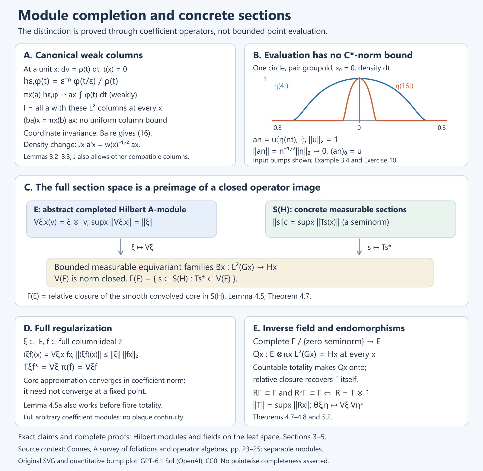
Open full-size figure · Open editable SVG

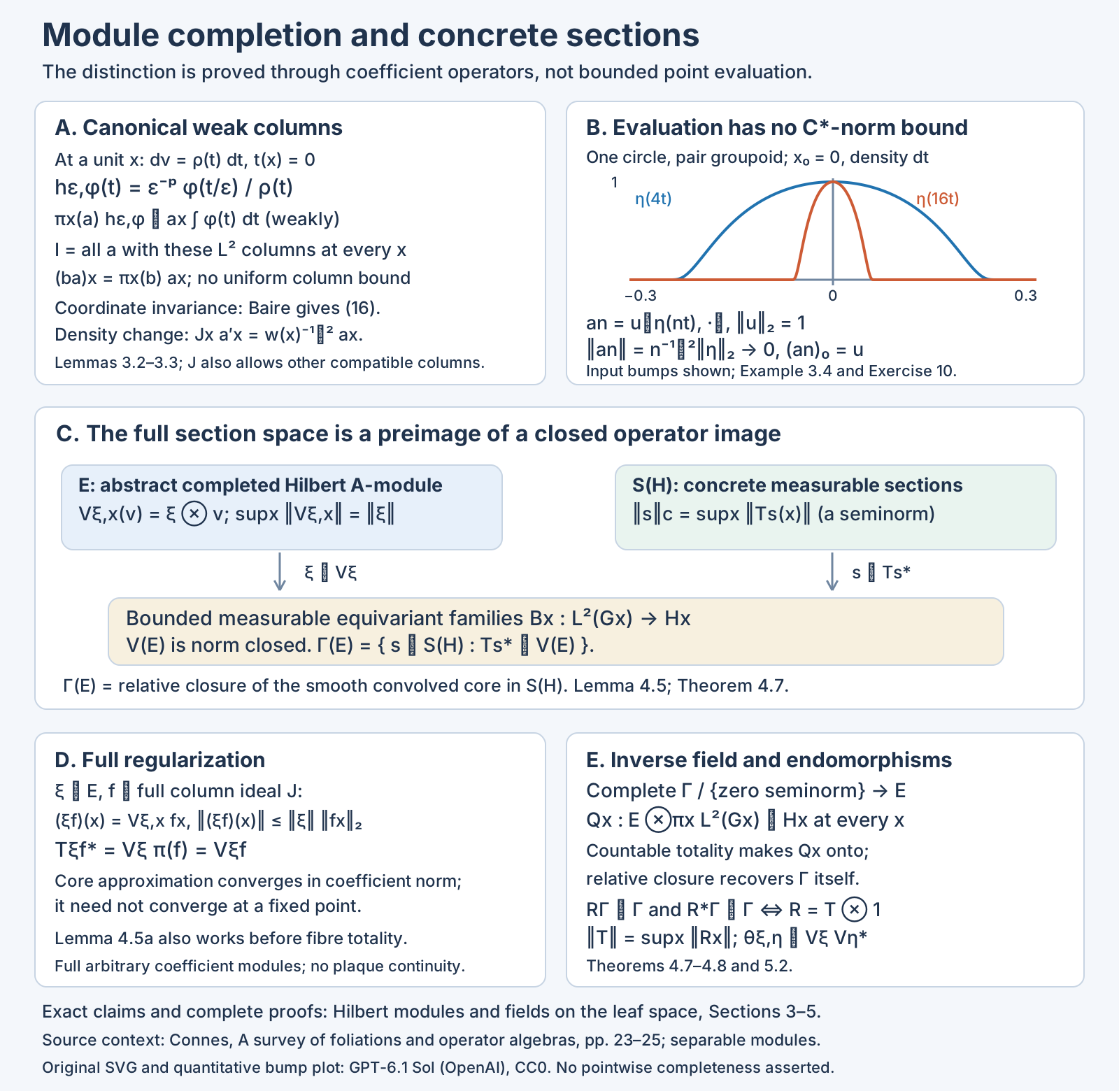
Figure 4.8. The maps and norms of Lemmas 3.2–3.3 and 4.5–4.5a, Theorems 4.7–4.8 and Theorem 5.2. The upper-right plot is the input bump of Example 3.4 for \(n=4,16\), in the coordinate \(t\in[-0.3,0.3]\), with \(x_0=0\) and leaf density \(dt\). Here the plotted sample is \(\eta(z)=\exp(1-(1-z^2)^{-1})\) for \(|z|<1\), and zero outside; each \(\eta(nt)\) equals one at zero while its \(L^2\) norm is \(n^{-1/2}\|\eta\|_2\). The statements below the plot hold for every smooth compact input bump with \(\eta(0)=1\). The middle panel identifies the concrete section space as the preimage of the norm-closed operator image \(V(E)\). The arrows do not give a value of every \(\xi\in E\) at a point. The lower panels state the full-column regularization, coefficient completion after quotient, all-point fibre recovery and exact endomorphism norm. For the canonical weak-column choice, restore endpoint half-densities as in (17); for another full admissible ideal use its given compatible columns. Complete arguments accompany the figure. Primary source: [Connes], PDF pages 23–25, in the separable-module context.

5. Endomorphisms and strict convergence

Lemma 5.1. If \(E\) is countably generated, \(\mathcal K_A(E)\) has a positive contractive sequential approximate identity \(e_n\) that also satisfies \(e_n\xi\to\xi\) for every \(\xi\in E\).

Proof. Choose generators \(\xi_j\) of norm at most one, and set

The series converges in norm. Since \(\theta_{\xi_j,\xi_j}\le2^jh\),

The last bound is the maximum of \(t n^{-2}/(t+n^{-1})^2\). Thus \(e_n\) tends to the identity on every generator, and boundedness extends this to their dense module span. The formulas for rank-one operators show that \(e_nS\to S\) and \(Se_n\to S\) in norm for every \(S\in\mathcal K_A(E)\). \(\square\)

For each adjointable \(T\), \(Te_n\) is compact and \(\|Te_n\|\le\|T\|\). Moreover \(Te_n\xi\to T\xi\) and \((Te_n)^*\xi=e_nT^*\xi\to T^*\xi\). This is strict convergence.

These approximations also prove the multiplier description \(\mathcal L_A(E)=M(\mathcal K_A(E))\). Write \(K=\mathcal K_A(E)\). An adjointable operator multiplies \(K\) on both sides by the rank-one formulas in Section 1. This multiplier determines the operator uniquely, since \(Te_n\xi\to T\xi\). Conversely let \(m\in M(K)\). The compact operators \(me_n\) have norm at most \(\|m\|\). On a vector \(S\xi\), with \(S\in K\),

The linear span of these vectors is dense in \(E\), because it contains every \(e_n\xi\). The common norm bound extends this convergence to every vector of \(E\), giving a bounded module operator \(T_m\). The adjoints \((me_n)^*=e_nm^*\) converge on the same dense span to \(T_{m^*}\): on \(S\xi\) their limit is \((m^*S)\xi\). Passing to the limit in the inner-product identity proves \(T_m^*=T_{m^*}\). Moreover \(T_mS=mS\) and \(ST_m=Sm\), using \(e_nS\to S\) and \((Sm)e_n\to Sm\). Thus every multiplier comes from exactly one adjointable operator. The correspondence is a faithful *-isomorphism and hence isometric. [Meyer] gives a general account of this identity.

Call a bounded measurable equivariant operator family \(R_x\) continuous when \(R\Gamma\subset\Gamma\) and \(R^*\Gamma\subset\Gamma\), for the entire closed concrete section space of Definition 4.6, or for any field satisfying the four axioms of Theorem 4.7. No extra preservation condition on an unspecified completion is part of this definition.

Theorem 5.2. There is an isometric *-isomorphism between \(\mathcal L_A(E)\) and the continuous equivariant operator families on the associated field. It takes \(T\) to \(T_x=T\otimes1\). Compact module operators correspond to the norm closure of the equivariant rank-one section operators.

Proof. If \(T\in\mathcal L_A(E)\), set \(T_x=T\otimes1\). Its measurability and equivariance follow on elementary tensors and then by density. For every \(s\in\Gamma(E)\) representing \(\xi\), equivariance in the coefficient formula gives

Hence both \(T_x\) and its adjoint preserve the entire relatively closed section space. Section 2 proves \(\|T\|=\sup_x\|T_x\|\).

Conversely let \(R_x\) be a bounded measurable equivariant family such that \(R\Gamma\subset\Gamma\) and \(R^*\Gamma\subset\Gamma\). The same coefficient identity gives \(\|Rs\|_{\mathrm c}\le(\sup_x\|R_x\|)\|s\|_{\mathrm c}\), and \(c_{Rs,t}=c_{s,R^*t}\). It therefore respects zero seminorm, extends to a bounded operator \(R_E\) on the completed module, and has adjoint \((R^*)_E\). Equivariance gives \(R(s*f)=(Rs)*f\) by the weak integral, or by \(T_{Rs}^*=R_xT_s^*\). Thus it is \(A\)-linear on the dense core and on its completion.

Under the full inverse isometry of Theorem 4.8, for every \(s\in\Gamma\),

Since \([\Gamma]\) is dense in \(E\), this holds for every module vector. The vectors \(V_{\xi,x}v=\xi\otimes v\) span a dense subspace in each tensor fibre. Thus \(R_x=R_E\otimes1\) at every \(x\). This proves surjectivity, uniqueness and the exact norm equality for arbitrary fields having the four axioms, rather than only for the smooth-core construction.

Finally the operator induced by \(\theta_{\xi,\eta}\) is \(V_{\xi,x}V_{\eta,x}^*\). Indeed on \(\zeta\otimes v\) it is \(\xi\otimes\pi_x(\langle\eta,\zeta\rangle)v\). For concrete sections it is \(T_s(x)^*T_t(x)\). Finite spans and their norm closures identify the compact algebras. This fixes the order of the two entries under our inner-product convention: \(\xi\langle\eta,\cdot\rangle\) corresponds to \(T_s^*T_t\), while \(\eta\langle\xi,\cdot\rangle\) corresponds to its adjoint. The source prints the latter module formula for the former operator; with its stated first-variable antilinearity the order must be corrected as above. Their compact span and the endomorphism theorem are unaffected. The multiplier description preceding the theorem then gives \(\mathcal L_A(E)=M(\mathcal K_A(E))\). \(\square\)

Lemma 5.3 (boundedness of strict sequences). Every strictly convergent sequence \(T_n\) in \(\mathcal L_A(E)=M(\mathcal K_A(E))\) is uniformly bounded in operator norm.

Proof. For every \(S\in\mathcal K_A(E)\), \(T_nS\) converges in norm and is therefore bounded. Apply the uniform boundedness principle to the bounded maps \(L_n:S\mapsto T_nS\) on the Banach space \(\mathcal K_A(E)\). It gives \(\sup_n\|L_n\|<\infty\). Moreover \(\|L_n\|=\|T_n\|\): the upper bound is immediate, while \(T_ne_j\xi\to T_n\xi\) for the approximate identity of Lemma 5.1 gives \(\|T_n\|\le\sup_j\|T_ne_j\|\le\|L_n\|\). This argument is for sequences; a convergent net need not have a bounded entire index set. \(\square\)

Corollary 5.4. A strictly convergent sequence \(T_n\) gives a strongly convergent sequence \((T_n)_x\) in every canonical tensor fibre.

Proof. For \(\xi\otimes v\),

Finite sums are dense and Lemma 5.3 gives uniform boundedness. This proves strong convergence. The same reasoning with adjoints gives strong convergence of adjoints. More generally the argument holds in any nondegenerate representation of \(\mathcal K_A(E)\): its dense vectors are \(S_xv\), and strict convergence gives norm convergence of \((T_n)_xS_xv\).

For a field with a countable total family as above, that representation is nondegenerate. Indeed its compact rank-one operators have the form \(T_s(x)^*T_t(x)\). The span of their ranges has the same closure as the span of the ranges of \(T_s(x)^*\), since \(\overline{\operatorname{ran}B^*B}=\overline{\operatorname{ran}B^*}\) for a bounded Hilbert-space operator \(B\). The orthogonality argument in Theorem 4.2 proves that this span is dense in \(H_x\). Thus the conclusion also applies directly to the continuous operator families used in the coefficient construction. \(\square\)

6. Sobolev modules and the analytic symbol class

The stable boundary construction used in formulas (11)–(13) is proved in The index map and the exact sequence at \(K_0\), Theorem 2.2 and Proposition 5.1, with kernel-minus-cokernel sign. The identification of the full compact-pair symbol group with stabilized bundle triples is Topological K-theory of spaces, pairs and vector bundles, Theorem 2.1, Lemma 2.2 and Section 3. The arguments below prove the longitudinal operator and symbol comparison for those classes.

The following construction uses the compact-support longitudinal calculus proved in the index lesson, Lemmas 6.1–6.8. Its finite-chart version, Proposition 6.21, permits non-Hausdorff arrows. Compactness here always means module compactness. An inclusion of Sobolev spaces on an infinite cover can fail to be a compact Hilbert-space operator.

Let \(B\to V\) be a finite-rank Hermitian bundle and keep \(V\) compact. Fix a positive leafwise density when expressing kernels and formal adjoints. Embed \(B\) isometrically into a trivial bundle \(V\times\mathbb C^N\), and let \(p_B\in M_N(C(V))\) be its orthogonal projection. Such an embedding follows from finitely many local frames and a partition of unity: their weighted components give an injective bundle map, and multiplication by the inverse square root of its positive Gram matrix makes it isometric. Multiplication by \(p_B(r(\gamma))\) on range-fibre kernels defines a multiplier of \(M_N(A)\). Put

Its canonical tensor fibre is \(L^2(G_x;r^*B)\). This follows by sending a column of chart kernels tensored with a fibre vector to its regular convolution; the inner products agree, and chart vectors are total. Different bundle embeddings give isometrically isomorphic modules through the corresponding bundle isometry. Direct calculation with rank-one operators gives

Indeed a rank-one map is a matrix product of one column with the adjoint of another. Such products span the displayed corner densely, by an approximate identity of \(A\).

A resolvent inside the algebra

Lemma 6.1 (multipliers and a parameter inverse). Every compactly supported longitudinal operator of order zero between bundles induces an adjointable map between the corresponding modules \(\mathscr E_B^0\). Negative-order operators give compact module maps. If \(\Delta_B=\nabla^*\nabla\ge0\) is the longitudinal connection Laplacian, then

is a positive injective module operator with dense range. Its represented operator is the stated spectral resolvent in every holonomy cover.

Proof. An order-zero operator \(P\) takes a compact smooth arrow kernel to a compact smooth arrow kernel by composition. The uniform represented bound gives

The same is true of the formal adjoint, and the kernel pairing gives the module-adjoint identity on this dense core. Extension gives the adjointable map. For negative order, the frequency truncation proof in Lemma 6.2 of the index lesson places its bundle matrix in the corner (3).

We supply the parameter estimate needed for the resolvent rather than inferring it from fibrewise inverses. For \(\lambda\ge1\), set

In each of finitely many protected plaque charts, the leading inverse symbol of \(\lambda+\Delta_B\) is

Uniform metric positivity and differentiation of the inverse give

Here and below only leafwise derivatives are taken; their constants are uniform in the transverse parameter. In the exact differential-symbol product, cancel the error of parameter order minus one by multiplying its symbol on the left by \(q_{-2}\). Repeat to cancel the next order. After \(M\) steps the successive symbols have bounds

The finite Taylor formula for composition proves these bounds by induction: a frequency derivative lowers parameter order by one, a first-order coefficient has order one, and a zeroth-order coefficient has order zero. The principal scalar inverse commutes with the bundle matrices; their lower-order products need no commutativity. Patch the finite inverse with fixed near-unit cutoffs. Correct the overlap and cutoff errors by the same successive order cancellation. The resulting \(Q_{\lambda,M}\in\Psi_c^{-2}\) has left and right errors of arbitrarily prescribed negative parameter order, by taking \(M\) large enough.

There are also separated-cutoff errors. They decay faster than every power of \(\lambda\): on their support \( |x-y|\ge d>0\), transfer \(k\) derivatives onto the symbols with the Fourier phase. The absolute frequency integral is bounded by

Any fixed number of input or output derivatives is accommodated by increasing \(k\). Finite chart sums preserve these bounds. For the diagonal errors, the Fourier–Schur estimate applied to (5) bounds their norms by \(C\lambda^{-a}\), for any prescribed \(a\), when sufficiently many terms have been cancelled. The same argument, conjugating in the coordinate Fourier norms, holds on each prescribed finite list of Sobolev orders. Thus for sufficiently large \(\lambda\) the right error

has norm less than \(1/2\). Both \(Q_{\lambda,M}\) and \(E_{\lambda,M}\) belong to the matrix corner of \(A\), while \(1+E_{\lambda,M}\) is an invertible multiplier. Therefore

In every fibre this is a right inverse of \(\lambda+\Delta_B\). The established differential-domain theorem and positivity identify it with the spectral inverse. Faithfulness of the family reflects positivity and its bound \(\|R_{B,\lambda}\|\le\lambda^{-1}\). For \(\lambda>1\), the resolvent identity gives

The second inverse is a norm-convergent geometric series since

\(\|(\lambda-1)R_{B,\lambda}\|\le1-1/\lambda<1\).

This proves compactness and identifies every fibre of \(R_B\). A zero vector in its module kernel is zero in every tensor fibre, hence is zero by faithfulness. Its range contains each compact smooth bundle kernel \(f\): the kernel \( (1+\Delta_B)f\) is in the module, and the spectral identity gives

These kernels are dense in \(\mathscr E_B^0\). Hence the range is dense. Every argument uses fixed finite arrow charts and their component estimates, so the non-Hausdorff extension applies. \(\square\)

Lemma 6.2 (powers with their symbol and continuity). The inverse of \(R_B\) is a positive regular self-adjoint module operator \(A_B=1+\Delta_B\). For every \(r>0\), \(A_B^{-r}\in\mathcal K_A(\mathscr E_B^0)\) has dense range. Its longitudinal symbol has order \( -2r\), with principal symbol \( |\xi|_g^{-2r}I_B\). More precisely, at every desired finite negative remainder order it is a compactly supported pseudodifferential operator of that order plus an error whose sufficiently differentiated kernels converge in the norm of the matrix algebra over \(A\). These errors may have noncompact arrow support. For every longitudinal \(P\in\Psi_c^m(B_0,B_1)\) and real \(s\),

extends to an adjointable order-zero multiplier. If \(m<0\) and the same normalization uses \(s\) in both modules, that multiplier is compact. The statements persist for continuous changes of metric or connection.

Proof. Define \(A_B=R_B^{-1}\) on \(\operatorname{ran}R_B\). It is closed, symmetric and positive, in fact bounded below by one. Its two resolvents are

They are adjoints of one another and have the required inverse identities. This proves self-adjointness and regularity: the positive operator \(1+A_B^2\) has inverse \(R_B^2(1+R_B^2)^{-1}\), and maps into the domain of \(A_B^2\). Thus \(1+A_B^2\) is onto, proving regularity. The tensor resolvents agree with the spectral resolvents on every cover. Bounded powers below are continuous functions of \(R_B\); their unbounded inverses are defined on their dense ranges. Thus only bounded C*-functional calculus is needed for this construction, and its represented powers agree with the ordinary spectral calculus.

Continuous functional calculus gives \(A_B^{-r}=R_B^r\in A\). Its range is dense. To see this directly, \(R_B(R_B+\varepsilon)^{-1}\) tends strictly to one because it does so on the dense range of \(R_B\), with uniform norm at most one. A sufficiently high integer power of this approximate identity factors through \(R_B^r\); thus the closure of the latter's range is the whole module.

For \(0<r<1\), the symbol and remainder assertion follows from the norm-convergent integral

The scalar identity is obtained by substituting \(t=au\) in the integral for \(a^{-r}\); the remaining beta integral is \(\pi/\sin\pi r\). Spectral calculus proves (8). At zero the norm integrand is bounded by \(t^{-r}\), and at infinity by \(t^{-r-1}\).

Integrate the finite parameter-symbol construction (5), with \(\lambda=1+t\). The estimates needed to differentiate under the integral are

Substitution \(t=\langle\xi\rangle^2u\) proves (9), and the integrated leading term has principal symbol \( |\xi|_g^{-2r}I_B\). Each further cancelled parameter order gives a further negative symbol order.

We justify the algebra norm of the remainders after differentiation. At large \(\lambda\), expand (6) as its Neumann series. Given differential operators \(L\) on the output and \(L'\) on the input, choose the cancelled order beyond their two orders and beyond the desired decay exponent. The term with one error factor, \(LQ_{\lambda,M}E_{\lambda,M}L'\), is then of sufficiently negative order. For \(k\ge2\), factor a differentiated correction term as

The outside factors have parameter-symbol bounds with arbitrarily large decay, while the middle factors have norm below \(1/2\). Every such term is a finite compact-support composition and belongs to \(A\) by negative-order frequency truncation. Its norm is bounded by \(C2^{-k}\lambda^{-b}\), with the constant absorbing the first two terms and \(b\) made as large as required. The Fourier–Schur estimate proves the bound in the represented algebra norm. Thus the differentiated series converges in \(A\), not just on each fibre. Increasing the cancelled order gives any prescribed finite differentiation and decay bound, sufficient for its integral in (8).

For \(\lambda\) in a bounded positive interval, use a fixed large \(\Lambda\) and

Its contraction ratio is at most \(1-\lambda_0/\Lambda<1\) when \(\lambda\ge\lambda_0>0\). After extracting finitely many factors of \(R_{B,\Lambda}\), the same series converges after the prescribed input and output derivatives. Explicitly choose \(j,j'\) so that \(LR_{B,\Lambda}^j\) and \(R_{B,\Lambda}^{j'}L'\) have negative order. The finite parameter construction and its differentiated Neumann series put these two factors in \(A\). For \(k+1\ge j+j'\), the differentiated tail term factors as

Its norm is bounded by \(C\Lambda^{-(k+1-j-j')}\). Multiplication by \((\Lambda-\lambda)^k\) leaves a convergent geometric bound, uniformly for \(\lambda\) in the given interval. This proves convergence in \(A\) after both differentiations. Expanding a sufficiently long initial segment of (10) gives the usual symbol terms; the tail has any specified lower order. This proves the bounded-parameter remainder assertion without assuming transverse continuity of an unspecified inverse.

Integer powers, composition and (8) now prove the assertion for all \(r>0\). Positive powers can be written on their common smooth core as \(A_B^kA_B^{-(k-u)}\), where \(k>u\). Thus their principal symbol is \( |\xi|_g^{2u}\). In any product of powers and \(P\), choose the finite parameter expansions to an order beyond all derivatives that the product requires. Its principal symbol is the product of their principal symbols, and the remaining differentiated errors are norm limits in \(A\) as just proved. The total order of (7) is zero. Its compact-support symbol part is an adjointable multiplier by Lemma 6.1; its error and the corresponding adjoint error belong to \(A\). This proves (7), including its adjointability. If the total order is negative, frequency truncation makes the symbol part compact too. All finite estimates and series are uniform on a compact family of metrics or connections, and their terms are continuous in the parameter. Uniformly convergent series and integrals preserve that continuity. \(\square\)

The Sobolev fields

Theorem 6.3 (continuous Sobolev modules). For every real \(s\), there is a canonical Sobolev Hilbert module \(\mathscr E_B^s\) whose tensor fibres are

For negative \(s\) the fibre is the completion of \(L^2\) in this norm, equivalently its usual negative Sobolev space. The inclusion \(\mathscr E_B^{s'}\to\mathscr E_B^s\) is compact if \(s'>s\). Changing the auxiliary metric or connection induces an adjointable isomorphism of these modules by the natural distributional identification.

Proof. Take an abstract copy of \(\mathscr E_B^0\), and label its vectors in tensor fibres by the unitary

For \(s\ge0\) this is the inverse of the graph-norm isometry; for \(s<0\) it extends from its dense spectral domain to the indicated completion. The dense module domains of sufficiently high positive powers are available from regularity in Lemma 6.2, so the fibre labels are compatible with the measurable regularization structure. Spectral equivariance makes them commute with right transport. This defines \(\mathscr E_B^s\), together with its specific tensor-field identification, rather than trying to take pointwise values of every completed vector.

Under these identifications the inclusion for \(s'>s\) is represented on \(\mathscr E_B^0\) by \(A_B^{-(s'-s)/2}\in A\), hence is compact by (3). For another metric or connection, using the same reference density and Hermitian norm, the identity of distributions from its \(W^s\) to the first \(W^s\) is normalized by \(A_B^{s/2}(A'_B)^{-s/2}\). Lemma 6.2 makes it an adjointable order-zero multiplier; the reverse expression is its bounded inverse, first on the common smooth core and then by density.

Changing the density or Hermitian norm adds the corresponding smooth positive bundle multiplication. For example if the new density is \(w\) times the old one, the unitary from the new \(L^2\) to the reference \(L^2\) is multiplication by \(w^{1/2}\). Transport the new Laplacian by that unitary; the normalized identity of ordinary distributional sections then includes multiplication by \(w^{-1/2}\) between the two spectral powers. This is again an order-zero multiplier with the reverse identity as inverse. Compactness of \(V\) bounds these positive multipliers and their inverses. This proves continuity of the natural identifications, including the usual metric-volume convention. In every fibre the coordinate Sobolev comparison already proved in Theorem 6.8 of the index lesson identifies precisely these spaces, for all real orders. \(\square\)

Theorem 6.4 (elliptic module operators). Let \(D\in\Psi_c^n(B_0,B_1)\) be longitudinally elliptic. In particular \(D\) may be a differential operator using only leafwise derivatives. Then

is adjointable and invertible modulo compact module maps, for every real \(s\). Its fibre map is the stated differential or pseudodifferential Sobolev realization, including when the ordinary leafwise range is not closed.

Proof. Normalization gives exactly (7), which is adjointable by Lemma 6.2. A compact-support parametrix \(Q\in\Psi_c^{-n}\) exists by Theorem 6.3 of the index lesson, with both errors smooth compact arrow kernels. Normalize \(Q\) in the reverse Sobolev direction. The normalized errors have arbitrarily negative total order and belong to the appropriate matrix corner of \(A\). By (3) they are compact module operators. Thus \(D\) has a two-sided inverse in the quotient category by compact module maps, which is the definition of module Fredholmness. The density of the spectral smooth core and the fibre Sobolev theorem identify its fibre action with the closed Sobolev realization. No fibrewise Fredholm or closed-range assumption has entered. \(\square\)

Index invariance under symbols

For clarity, the projection-valued index can be constructed directly from such a parametrix. Write \(T:X\to Y\) and \(Q:Y\to X\) for the normalized maps, so \(QT-1_X,TQ-1_Y\) are compact. On the direct sums, form the invertible map \(W:X\oplus Y\to Y\oplus X\)

The first three matrices act on \(Y\oplus X\), and the last is the signed flip from \(X\oplus Y\). Thus every factor is invertible with the displayed types. If \(e_X\) projects onto the first summand of \(X\oplus Y\) and \(e_Y\) onto the first summand of \(Y\oplus X\), the idempotent \(P=W e_X W^{-1}\) differs from \(e_Y\) by a compact map. After embedding \(X=p_0A^{N_0}\), \(Y=p_1A^{N_1}\), extend \(P\) by the identity on the orthogonal complement of \(Y\) in the first trivial summand and by zero on the complement of \(X\) in the second. The resulting matrix idempotent differs from the constant projection \(e=\operatorname{diag}(I_{N_1},0_{N_0})\) by a matrix over \(A\). Consequently

Different finite bundle embeddings give the same class: place two isometric embeddings in separate trivial summands and join them by \(\cos\theta\,j_0\oplus\sin\theta\,j_1\), \(0\le\theta\le\pi/2\). This is an isometric bundle-embedding path, giving a continuous idempotent path after adding the same complements. Using idempotents or projections gives the same group. Explicitly the range projection of an idempotent \(P\) is

The denominator is positive and at least one. Relative to the orthogonal range decomposition, \(P=\left(\begin{smallmatrix}1&b\\0&0\end{smallmatrix}\right)\), which verifies the formula and its continuous dependence. The range projection is homotopic to \(P\) through idempotents by decreasing \(b\) to zero. The compact difference from the reference is retained throughout. Formula (12) is independent of \(Q\), since the straight path between two parametrices remains a parametrix and gives a continuous path of (11). It is additive under direct sums and invariant under norm-continuous Fredholm paths by the same formula. If \(T\) is invertible, use \(Q=T^{-1}\); then \(W=\operatorname{diag}(T,Q)\), \(P=e_Y\), and its index is zero. On finite Hilbert spaces the formula gives \(\dim X-\dim Y=\dim\ker T-\dim\ker T^*\), fixing its sign.

Lemma 6.5 (the longitudinal symbol quotient). Let \(\overline\Psi^0\) be the represented-norm closure of scalar compact-support classical order-zero longitudinal operators on the compact unit manifold, including \(A\). Then there is an exact sequence

The quotient norm is the supremum norm of the principal symbol. Bundle matrix corners have the corresponding assertion.

Proof. Composition and adjoints induce multiplication and adjoint on leading symbols. For a classical order-zero operator \(P\), put \(c=\sup\|\sigma(P)\|\). Quantize the positive matrix square root of

\((c^2+\varepsilon)I-\sigma(P)^*\sigma(P)\)

as an order-zero \(B\). A uniformly convergent differentiated binomial series constructs this square root, since the positive spectrum stays uniformly away from zero. The calculus gives

In the multiplier quotient this implies \(\|P+A\|\le\sqrt{c^2+\varepsilon}\); let \(\varepsilon\downarrow0\).

For the opposite inequality, choose a point and covector on the unit cosphere and an input bundle vector. In one protected lifted plaque take a unit wave packet supported in a ball of radius \(h^{1/2}\), with phase \(e^{i\langle x,\xi\rangle/h}\). Taylor expansion in its Fourier integral shows

For details, rescale \(x=x_0+h^{1/2}z\); the packet's frequency is \(\xi_0/h+O(h^{-1/2})\), so degree-zero homogeneity and continuity give convergence on bounded rescaled frequencies. The rapidly decreasing Fourier tails of its fixed smooth bump, with the order-zero bound, give dominated convergence on the complement. Off-diagonal smooth pieces tend to zero by integration by parts in the oscillatory input. Every compact smooth arrow kernel also takes \(u_h\) to a vector tending to zero, by that argument on finitely many chart components. Uniform represented-norm approximation gives the same assertion for every \(a\in A\). Hence \(\|P+a\|\ge\|\sigma(P)(x_0,\xi_0)\|\). Taking suprema proves \(\|P+A\|=c\).

Smooth principal symbols are uniformly dense in \(C(S^*F)\), and quantization realizes them. The quotient-norm identity therefore extends the symbol map to the norm closure and makes its induced quotient isometric onto \(C(S^*F)\). Its kernel is precisely \(A\). More explicitly, a norm limit with zero symbol can be approximated by operators whose quotient norms tend to zero, and then by their corrections in \(A\). Negative-order membership supplies the initial kernel, and the norm identity prevents a new kernel in completion. All wave packets and symbol computations lie in a near-unit Hausdorff chart; other chart components are smooth there. Thus the argument also covers non-Hausdorff arrows. \(\square\)

Theorem 6.6 (dependence on the compactly supported symbol class). The analytic index of Theorem 6.4 is independent of \(s\), of the metric and connection, and of all lower-order terms. It depends only on

It is the index boundary supplied by (13), interpreted for bundle symbols. Identifying \(F^*\cong F\) by a metric gives the equivalent notation \(K_c^0(F)\); changing that metric gives a homotopic identification.

Proof. With the same tangent metric for both bundles, the normalized principal symbol in (7) is

independent of \(s\). Lemma 6.2 and the symbol construction show that every normalization differs from a compact-support order-zero quantization of this symbol by a compact module map. Operators with this same principal symbol differ by a compact map by (13). Their straight-line path remains invertible modulo compacts, so (12) gives the same index. A change of metric or connection gives the isomorphisms of Theorem 6.3, and its symbol changes only through positive scalar factors and their invertible homotopy. Formula (12) is unchanged under such isomorphisms and homotopies.

Here is the full passage from a symbol to its K-theory class. Use the disk/sphere definition \(K_c^0(F^*)=K^0(BF^*,S^*F)\): a relative triple consists of two bundles over the disk bundle and an isomorphism of their restrictions to the sphere. Addition is direct sum; homotopy and triples whose isomorphism extends invertibly to the disk generate the equivalence relation. Every bundle over the disk is isomorphic to a pullback bundle from \(V\). To see this without a triviality assumption, embed it as a projection in a finite trivial bundle and contract the disk radially. Divide that contraction into finitely many pieces on which the projection changes by norm less than one; the isomorphism \(qp(pqp)^{-1/2}\) between the corresponding ranges transports the bundle at each step. This gives the required bundle isomorphism.

Thus every relative triple has the form of a bundle elliptic symbol used above. Smooth approximation makes its isomorphism smooth on the compact sphere and retains invertibility. The same can be done uniformly over a homotopy. Quantizing a smooth homotopy with fixed charts and cutoffs gives an operator-norm-continuous path, by the finite-seminorm Fourier–Schur estimate; quantize the inverse symbols to obtain its continuous parametrices. Equation (12) is consequently constant along it and additive under sums. Different approximations are joined through sufficiently small invertible perturbations, so give the same index.

If a sphere isomorphism extends invertibly to the disk, radial contraction of that extension homotopes it to an isomorphism over \(V\) alone. At that endpoint multiplication by the bundle isomorphism is an invertible module map, whose index is zero. Hence every relation defining the relative K-group preserves the index. This proves that the assignment descends to \(K_c^0(F^*)\), rather than merely to a homotopy class of differential operators of fixed order. Formula (11) is the explicit boundary lift of a quotient isomorphism and its inverse; thus (12) also proves agreement with the symbol exact sequence (13).

When the leaf dimension is zero, \(A=C(V)\), \(\mathscr E_B^s\) is the finite bundle module for every \(s\), and every module map between these modules is compact. The cosphere is empty. The relative triple is then just the difference of its two bundles; (12) gives \( [B_0]-[B_1]\). This is the same assertion in \(K_c^0(F^*)=K^0(V)\). It handles this case without a nonexistent unit covector. \(\square\)

This proves the analytic symbol-class map. Identifying it with a geometrically defined topological pushforward is the further longitudinal index theorem; its Thom and deformation arguments are developed in the K-theory lesson and remain separate from (13).

Example 6.7. For a product foliation with transverse base \(T\), the algebra is \(C_0(T)\otimes\mathcal K\). A compactly supported continuous field of finite-rank plaque kernels is a compact module operator. If a leaf is an infinite covering and its kernel repeats on all sheets, the represented operator can have infinite ordinary rank and need not be compact on that cover. In Theorem 6.3 the compact Sobolev inclusion belongs to the algebra through its global uniform approximation; no ordinary compactness on an infinite cover is asserted.

7. Exercises

Exercise 1 (basic). For the Hilbert module \(E=A\), show that \(\mathcal K_A(A)=A\), acting by left multiplication, and \(\mathcal L_A(A)=M(A)\).

Solution. The inner product is \(\langle a,b\rangle=a^*b\), and \(\theta_{a,b}\) is left multiplication by \(ab^*\). Products of this form span a dense subspace of \(A\), as an approximate identity shows, so the compact algebra is \(A\). The multiplier description in Section 5 gives the adjointable algebra. A multiplier is required when \(A\) is nonunital; left multiplication by an element of \(A\) does not give every adjointable endomorphism.

Exercise 2 (intermediate). Let \(A=C_0((0,1))\) and \(E=A\). Is multiplication by the constant function one compact as a module map? Is its operator on each one-dimensional fibre compact?

Solution. It is the identity multiplier, which is not in \(C_0((0,1))\), so it is not compact as a module map. Every fibre is one-dimensional and its identity is a compact Hilbert-space operator. Thus fibrewise compactness alone does not imply compactness of a module map.

Exercise 3 (intermediate). Verify the bound \(\|s_{\xi,f}(x)\|\le\|\xi\|\|f_x\|\), and explain why it does not give a bounded evaluation map \(E\to H_x\) without fixing \(f\).

Solution. Its squared norm is \(\langle f_x,\pi_x(\langle\xi,\xi\rangle)f_x\rangle\), bounded by \(\|\xi\|^2\|f_x\|^2\). The factor \(\|f_x\|\) is part of the estimate and need not be controlled by the C*-norm of \(f\). In a pair groupoid, take \(f_n(t',t)=g(t')a_n(t)\), with \(a_n(x)=1\) but \(\|a_n\|_2\to0\). Then \(\|f_n\|_r\to0\), while their columns at \(x\) remain \(g\). Evaluation on the whole completion cannot follow from this estimate.

Exercise 4 (advanced). Prove the generator estimate in Lemma 5.1, including its constant.

Solution. Apply \(1-e_n\) on both sides of \(\theta_{\xi_j,\xi_j}\le2^jh\). Its left side becomes \(\theta_{(1-e_n)\xi_j,(1-e_n)\xi_j}\), whose norm is \(\|(1-e_n)\xi_j\|^2\). Functional calculus reduces the right-side norm to \(2^j\sup_{t\ge0}t\varepsilon^2/(t+\varepsilon)^2\), with \(\varepsilon=n^{-1}\). Differentiation, or \((t+\varepsilon)^2\ge4t\varepsilon\), gives its maximum \(2^{j-2}\varepsilon\).

Exercise 5 (advanced). Let \(T_n=Te_n\) as in Section 5. Prove fibrewise strong convergence without claiming operator-norm convergence on the fibres.

Solution. The elementary tensors satisfy the estimate in Corollary 5.4 and hence converge. Uniform boundedness by \(\|T\|\) extends convergence to every vector. Norm convergence need not hold: on an infinite-dimensional Hilbert space, finite-rank approximations of the identity converge strongly but their norm distance from the identity stays one.

Exercise 6 (advanced). Consider an irrational linear flow on the two-torus, so each holonomy cover is \(\mathbb R\). For its longitudinal Laplacian \(-d^2/dt^2\), find the kernel of the resolvent at one. Prove that it is compact as an endomorphism of the standard foliation module but is not a compact operator on \(L^2(\mathbb R)\).

Solution. The kernel is \(k(t)=\tfrac12e^{-|t|}\). It solves \((1-d^2/dt^2)k=0\) away from zero and has derivative jump minus one there; hence the distributional equation is \((1-d^2/dt^2)k=\delta_0\). Fourier transformation gives multiplier \((1+\xi^2)^{-1}\), identifying the spectral resolvent. Smooth compactly supported approximations to \(k\) converge in \(L^1\). For the action groupoid of this flow, the convolution Schur bound bounds their reduced-norm error by that \(L^1\) error. Thus the resolvent belongs to \(A=C_r^*(V,F)\), which equals \(\mathcal K_A(A)\).

Choose a nonzero compactly supported vector \(v\), and let \(v_n(t)=v(t-n)\). These bounded vectors tend weakly to zero: first test against compactly supported vectors, where the pairing is eventually zero, and then use their density in \(L^2\). The resolvent commutes with translation and is injective, so \(\|Rv_n\|=\|Rv\|>0\) for all \(n\). A compact Hilbert-space operator sends a bounded weakly null sequence to a norm-null sequence, as follows by taking a convergent image subsequence and testing its limit against adjoint vectors. This contradiction proves that this represented resolvent is not compact.

Exercise 7 (intermediate). In (11), set \(T=Q=0\) for \(X=\mathbb C^3\), \(Y=\mathbb C^2\). Verify the index sign without an invertibility assertion about \(T\).

Solution. Finite-dimensional operators are compact, so zero is invertible in the quotient category, whose objects here have zero identity. The map \(W\) is the signed flip \((x,y)\mapsto(-y,x)\), an invertible map from \(X\oplus Y\) to \(Y\oplus X\). Thus \(P=\operatorname{diag}(0_Y,I_X)\), while the reference is \(e_Y=\operatorname{diag}(I_Y,0_X)\). Their rank difference is \(3-2=1\), equal to \(\dim\ker T-\dim\ker T^*\). The example checks that the parametrix formula uses kernel minus cokernel.

Exercise 8 (intermediate). In the one-leaf circle example, let \(s\) be a measurable half-density section of the regular field supported at one base point \(x_0\). Show that its coefficient seminorm is zero even when \(s(x_0)\ne0\). Explain why this does not contradict the all-point uniqueness of the canonical product section in (22).

Solution. For each \(x\), the pair-groupoid fibre is the circle, and the coefficient function \((T_s(x)v)(\gamma)\) vanishes except where \(r(\gamma)=x_0\). This is one point of the fibre, hence has zero leaf measure. Thus every \(T_s(x)\) is zero and (23) vanishes. A relative closed section space contains all these zero-distance modifications; the abstract module quotients them. In contrast (22) takes weak distributional columns of a specified operator. A zero operator has zero weak column at every unit by (15). It chooses the zero representative, rather than an arbitrary modification supported at one point. Operator classes and their canonical regularized representatives answer different questions.

Exercise 9 (advanced). Show that replacing weak by strong convergence in (15) would give a strictly smaller domain, already for compact operators on one circle.

Solution. Work near the coordinate point zero with density \(dt\). Choose \(0\le\eta\le1\) smooth, equal to one on \([1,2]\), supported in \((3/4,5/2)\). Put \(\varepsilon_n=4^{-n}\), \(v_n(t)=\eta(t/\varepsilon_n)\), and choose smooth orthonormal output vectors \(u_n\) in \(L^2(S^1)\). The input supports are disjoint. The series

converges in operator norm: its tail norm is \(\sup_{n>N}\|v_n\|_2 =\varepsilon_{N+1}^{1/2}\|\eta\|_2\to0\). Thus \(B\) is compact. Away from zero its input column is locally the smooth vector \(v_n(t)u_n\), or zero, so has a strong point value. At zero the column is weakly zero. To see this, its averages against a rescaled fixed test have norm at most \(\|\varphi\|_1\), by the disjoint supports and \(\|u_n\|=1\). For sufficiently small radii all their components have arbitrarily large indices. Pairing with any fixed vector therefore tends to zero: first approximate that vector by a finite combination of the \(u_n\), and then use the uniform bound. This proves (15) for every test at zero.

Choose an integral-one test supported in \((1,2)\). At radius \(\varepsilon_n\), its average sees only the region where \(v_n=1\), and equals \(u_n\). Its norm is one. It cannot converge strongly to the weak limit zero. Hence \(B\in\mathcal I\), while the strong-column domain excludes it.

Exercise 10 (advanced). Suppose a concrete section \(s\) represents \(\xi\) in (25), and \(f_n\in\mathcal C\) tends to \(f\in\mathcal I\) in C*-norm. Prove convergence of \(s*f_n\) to \(s*f\) in coefficient norm. Does the conclusion imply convergence of their values at a fixed \(x\)?

Solution. Their coefficient operators are \(V_{\xi f_n}\) and \(V_{\xi f}\). The isometry (21) gives precisely (27), so relative closure applies because \(s*f\) is already a concrete measurable section. Values at a fixed point need not converge. Set \(E=A\) for the circle, take the operators \(a_n\) in (20), and choose \(\xi\) a smooth rank-one projection fixing \(u\). Then \(\xi a_n=a_n\to0\) in module norm while its canonical value at \(x_0\) is always \(u\). The missing uniform estimate is a bound for \(\|(a_n)_{x_0}\|\) in terms of \(\|a_n\|\), which (20) refutes.

References

• [Landsman] N. P. Landsman, Lecture notes on C*-algebras, Hilbert C*-modules, and quantum mechanics, draft of 8 April 1998, arXiv version 1, submitted 24 July 1998. Sections 3.2–3.3 and 3.5. Public draft.

• [Connes] Alain Connes, A survey of foliations and operator algebras, in Operator Algebras and Applications, Part I, Proceedings of Symposia in Pure Mathematics 38, American Mathematical Society, 1982. Author's text.

• [Kasparov] G. G. Kasparov, Hilbert C*-modules: theorems of Stinespring and Voiculescu, Journal of Operator Theory 4 \(1980\). Full text.

• [Meyer] Ralf Meyer, Hilbert C*-modules and correspondences, Cuntz–Pimsner algebras, notes from an unfinished book project. Author’s notes.