From rotated endpoint signs to subellipticity

The first nonzero rotated Hamilton derivative measures finite type. Its sign at an odd order must be a neighborhood condition, because a nearby adverse crossing can carry a concentrated approximate null solution. To prove sufficiency, we must also treat a zero that is infinitely flat along one chosen time curve. Finite bracket type does not make that particular time zero finite. Instead it supplies a transverse derivative, and the characteristic slope controls a nearby zero branch.

The exact rotated-bracket equivalence and multiplier endpoint formula are Theorem 5.1, Corollary 5.2 and Lemma 2.1 of Rotated brackets and finite-jet flow coordinates. Exact homogeneous complex preparation is Theorem 3.1 and Corollary 3.2 of Smooth complex preparation and conic flow coordinates. The necessary direction and the persistent minimum adverse root are Theorem 6.1 and Lemma 1.1 of Crossing direction and the necessary finite-type bound. Once the geometric hypotheses are normalized, the full analytic sufficient estimate is Theorem 1.1 and Corollary 7.1 of Recovering a conic norm from scaled frequency bands. We prove the geometric implication here, including flat time zeros, and assemble the full equivalence. Historical attribution is Hörmander [H, Theorem 27.1.11].

Throughout, \(D=-i\partial\) and \(H_fg=\{f,g\}\). A characteristic point is a point where both real and imaginary parts of the principal symbol vanish. A word's length counts its real leaves, not its Hamilton differentiations.

1. The full neighborhood criterion

Let \(P\) be scalar and properly supported, of real order \(m\), in the ordinary \(S_{1,0}\) calculus. Let \(p\) be its smooth homogeneous principal representative modulo symbols of order \(m-1\). Fix a nonzero covector \(c_0\) and \(0<\delta<1\). Write

Theorem 1.1. The following are equivalent.

1. For every real \(s\) and every distribution, \(Pu\in H^s\) at \(c_0\) implies \(u\in H^{s+m-\delta}\) there.
2. There is a common neighborhood \(V\) of \(c_0\) on which both conditions hold: at every \(c\in V\), some \(z\) and some integer \(j\leq K\) have \(T_j(z;p,c)\ne0\); if the least integer \(r\) for which \(T_r(z;p,c)\) is not identically zero as a function of \(z\) is odd, then \(T_r(z;p,c)\geq0\) for every \(z\).

Nonvanishing in the first condition can be checked at \(c_0\) and then continued to a smaller neighborhood. The odd endpoint orientation must hold at every point of a common neighborhood. These are distinct assertions. At an elliptic point the least order is zero, so the orientation condition has no odd endpoint to constrain.

For the normalized order-one symbol, bracket depth \(\kappa(c)\) means that all real-leaf words with at most \(\kappa(c)\) leaves vanish at \(c\), and some word with \(\kappa(c)+1\) leaves does not. At an elliptic point put \(\kappa=0\); allow infinite depth otherwise. Under the characteristic first-slope condition, the rotated-bracket equivalence identifies \(\kappa\) with the least nonzero rotated endpoint order.

2. Preserve the least endpoint while preparing the symbol

At a characteristic point,

If this bracket is nonzero, the least endpoint order is one and the hypothesis in Theorem 1.1 makes it positive. If it is zero, it is already nonnegative. Thus the hypotheses imply the characteristic first-slope condition throughout \(V\).

Lemma 2.1. The neighborhood hypotheses of Theorem 1.1 are preserved by a smooth nonzero complex multiplier and by a symplectic coordinate change. At a characteristic point satisfying those hypotheses, the complex Hamilton field of a degree-one representative cannot be a complex radial multiple.

Proof. A symplectic map preserves all brackets and their forward Hamilton flow parameters. For a multiplier \(a\ne0\), the first bracket at a characteristic point is multiplied by \(|a|^2\), so its nonnegativity persists. The rotated-bracket theorem applies to both symbols. The ideals generated by all words through each length have the same vanishing under the invertible real linear change of leaves induced by \(a\). Hence their bracket depths agree.

Let that depth be \(r<\infty\). All words with at most \(r\) leaves vanish. The finite product rule of the rotated-bracket lesson therefore freezes the multiplier in the first surviving endpoint:

The right argument ranges over every complex number as \(z\) does. Nonvanishing and, for odd \(r\), the sign of every endpoint are preserved. At a noncharacteristic point the least order remains zero. This proves the full multiplier assertion, including a multiplier of any real homogeneous order after its smooth nonzero restriction to the working cone.

Now let the symbol have homogeneous degree one. Suppose \(H_p(c)\in\mathbb C R_c\), where \(R\) is the cotangent radial field. For every constant \(z\), the real Hamilton field of \(F=\operatorname{Re}(zp)\) equals a real multiple \(a_zR\) at \(c\). Degree-one homogeneity makes that Hamilton field invariant under cotangent dilation. Its restriction to the ray is consequently \(a_zR\), and its curve through \(c\) is \(e^{a_zs}c\), with the constant curve included when \(a_z=0\). The homogeneous function \(\operatorname{Im}(zp)\) is zero on this entire ray, since it is zero at \(c\). Every \(T_j(z;p,c)\) is zero. This contradicts finite nonvanishing. ∎

For a degree-\(m\) symbol, multiply first by a positive elliptic homogeneous factor of degree \(1-m\). Lemma 2.1 preserves the endpoint criterion. The resulting degree-one symbol has the nonradial field just proved. Exact homogeneous preparation now gives a homogeneous symplectic chart and a nonzero multiplier in which

The marked point has \(t=x=\tau=0\), \(\eta=\eta_0\ne0\). The exact multiplier and coordinate construction, including its homogeneous extension from a radial slice, is the preparation lesson's Theorem 3.1. The endpoint conditions and finite type hold throughout a smaller working neighborhood by Lemma 2.1. In particular,

A characteristic finite endpoint cannot occur in dimension one. For a degree-one symbol there, Euler's identity at a nonzero characteristic covector gives its momentum derivative zero. Its Hamilton field is then radial, contrary to Lemma 2.1. The elliptic case will be treated separately. Thus (2.3) has at least one transverse canonical pair whenever it is needed.

3. At a flat time zero, a transverse jet must survive

Lemma 3.1. Suppose \(q(0,w_0)=0\), every pure time derivative \(\partial_t^jq(0,w_0)\) is zero, and the full real-leaf bracket depth of \(\tau+iq\) at \((0,0,w_0)\) is finite. Then some finite \(s\geq0\) and some transverse vector \(v\) satisfy

Proof. Suppose all such transverse differentials vanish. Put \(Q_j=\partial_t^j q\). Its time differential is also zero, by flatness of the next pure time jet, and its \(\tau\) differential is zero by independence of \(\tau\). Thus \(dQ_j=0\) and \(H_{Q_j}=0\) at the marked point for every \(j\).

Consider a right-nested word. If all its Hamilton factors are \(H_\tau=\partial_t\), it is a pure time derivative of \(q\), or a time derivative of \(\tau\), and vanishes at the point; the one-leaf words also vanish. Otherwise, before the first \(H_q\) encountered from the outside, there is a finite string \(\partial_t^r\). The remaining inner expression is some smooth \(B\). Repeated product differentiation, or the identity \([\partial_t,H_q]=H_{q_t}\), gives

Every term vanishes at the point, since its acting vector is zero. Hence every finite word vanishes, contradicting finite bracket depth. This proves (3.1). ∎

This argument proves existence of a transverse derivative, not existence of a nonzero pure time jet. The distinction is what permits the next lemma to include flat time zeros.

4. The characteristic slope controls a nearby flat branch

Lemma 4.1. Under the hypotheses of Lemma 3.1, suppose also that (2.4) holds in a neighborhood. Then, for some \(\epsilon>0\),

Identically zero portions are allowed. Thus an infinitely flat time zero cannot be the boundary of an adverse positive-to-negative transition under these hypotheses.

Proof. Choose the transverse line from Lemma 3.1, using a coordinate \(v\) along it and holding the other transverse variables fixed. Translate \(w_0\) to \(v=0\). Write \(Q(t,v)\) for the restricted function, and choose the least \(s\) for which \(\partial_t^s Q_v(0,0)=c\ne0\). Set \(c_*=c/s!\). Then

All estimates below are on a fixed small closed product neighborhood, where \(|Q_{vv}|\leq M\). For sufficiently small nonzero \(t\), \(|g(t)|\geq |c_*||t|^s/2\). On \(|v|\leq r(t)=|t|^{s+1}\), the difference between \(Q_v(t,v)\) and \(g(t)\) is at most \(M|t|^{s+1}\). Shrinking \(\epsilon\) makes this less than \(|c_*||t|^s/4\). Thus \(Q_v\) has the sign of \(c_*t^s\) throughout this short segment, and magnitude at least \(|c_*||t|^s/4\).

Flatness of \(f\) also gives, after shrinking again, \(|f(t)|<|c_*||t|^sr(t)/8\). The integral of \(Q_v\) from zero to either endpoint \(\pm r(t)\) therefore dominates \(f(t)\) in magnitude. The two endpoint values of \(Q(t,\cdot)\) have opposite signs. Strict monotonicity and the intermediate value theorem give a unique root \(v=a(t)\) in this segment. For \(t\ne0\), the implicit function theorem makes \(a\) smooth on each half interval. Moreover,

The points \((t,0,w(v=a(t)))\) are characteristic points of the full symbol. Equation (2.4) makes the numerator in the last expression nonnegative. On \(t>0\), the denominator has the fixed sign of \(c_*\), so \(c_*a'(t)\leq0\). Its continuous zero limit at zero gives \(c_*a(t)\leq0\). By the sign of \(Q_v\) on the segment joining \(a(t)\) to zero,

On \(t<0\), put \(c_-=(-1)^s c_*\). The denominator has this fixed sign, so \(c_-a'(t)\leq0\). Integrating toward its zero limit at zero now gives \(c_-a(t)\geq0\). The same integral has sign nonpositive, proving the left part of (4.1). No differentiability of \(a\) at zero was needed: its zero limit and monotonicity on each half interval suffice. ∎

The moving root is arbitrarily close to the original time curve because \(f\) is flat and the transverse slope loses only a finite power of \(t\). This supplies exactly the neighborhood characteristic points at which the slope condition can be used.

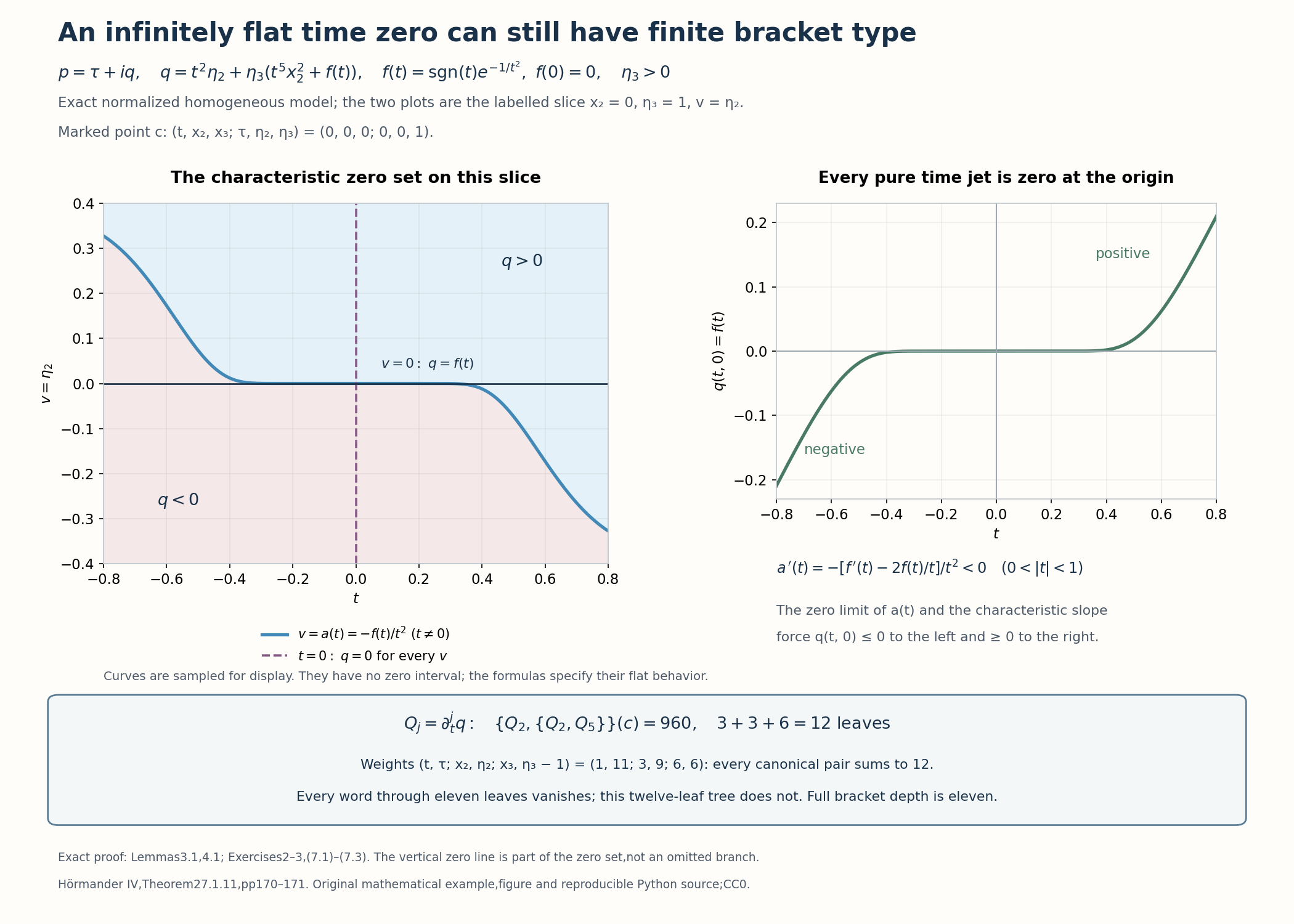
Figure 1. The exact example is (7.1), at \(c=(0,0,0;0,0,1)\). The plots are the labelled slice \(x_2=0,\eta_3=1,v=\eta_2\); the line \(t=0\) is part of the characteristic zero set for every \(v\), in addition to the punctured-time branch \(a(t)=-f(t)/t^2\). Its slope and side signs are Exercise 3 and the argument (4.2)–(4.4). Curves are numerical samples of the exact displayed functions; their visual overlap with zero near the origin does not represent a zero interval. The weighted lower vanishing and exact tree value are Exercise 2, (7.2)–(7.3). Historical source for the criterion: Hörmander [H, pp. 170–171]. Original mathematical example and CC0 figure; reproducible Python source.

5. A minimum adverse finite root contradicts the odd endpoint

Lemma 5.1. For the normalized symbol (2.3), the full neighborhood endpoint conditions imply that no time curve changes from positive to negative.

Proof. First exclude adverse zeros of finite odd order. If any such zero exists, choose the smallest odd order \(r\) occurring anywhere in the working neighborhood and a point where it occurs. The minimum-root lemma of the necessary-sign lesson gives, on a smaller product neighborhood,

At a point of this root branch put \(\tau=0\). We verify the lower word vanishing needed for the endpoint test. Write \((S^e)\) for smooth multiples of \(S^e\). Since \(H_\tau S=1\), \(H_\tau\) maps \((S^e)\) into \((S^{e-1})\), for \(e\geq1\). Since \(q=S^rb\), the product rule and \(\{S,S\}=0\) give

In particular \(H_q\) does not decrease a positive vanishing power. A word ending in the leaf \(q\) begins with power \(r\), and each Hamilton factor decreases it by at most one. Every such word with at most \(r\) leaves vanishes on the branch. For a word ending in \(\tau\), an innermost \(H_\tau\) makes it zero. The other possible innermost factor gives \(H_q\tau=-q_t\in(S^{r-1})\); at most \(r-2\) further factors leave a positive power. The one-leaf \(\tau\) vanishes by its chosen value. This proves vanishing of every word through \(r\) leaves. When \(r=1\), only the two leaves need vanish, which they do.

Every rotated endpoint of order less than \(r\) is a constant linear combination of words with at most \(r\) leaves, so is zero. But

Thus the least endpoint order is the odd integer \(r\), and its endpoint is negative. This contradicts the neighborhood orientation condition. No adverse finite odd root can exist.

It remains to rule out a transition without such a root. At a finite time zero, an even first nonzero derivative gives the same sign on its two punctured sides; an odd derivative must have positive coefficient by the preceding exclusion, and gives negative on the left and positive on the right. At an infinitely flat time zero, Lemmas 3.1 and 4.1 give the same permitted one-sided inequalities.

For a precise passage from these local assertions to a complete time interval, suppose \(f(t)=q(t,w)\) has \(f(t_1)>0\), \(f(t_2)<0\), \(t_1<t_2\). Put \(b=\sup\{t\in[t_1,t_2]:f(t)>0\}\). Continuity and the strict endpoint signs give \(t_1<b<t_2\), \(f(b)=0\), positive values arbitrarily close to \(b\) from the left, and no positive value in \((b,t_2]\). An odd positive or infinitely flat zero at \(b\) forbids those left positive values. A finite even zero with negative leading coefficient also forbids them. The only remaining case is a finite even zero with positive leading coefficient, which forces positive values immediately to its right, contrary to the supremum. This excludes the proposed transition, including isolated even zeros and zero intervals. ∎

6. Complete the conic estimate and the equivalence

Proof of Theorem 1.1. The necessary direction, including the common conic neighborhood, every rotated endpoint, the loss bound, all real orders and the indispensable nearby orientation, is Theorem 6.1 of the necessary-sign lesson. We prove the sufficient direction.

At an elliptic \(c_0\), a proper conic inverse of \(P\) gives \(u\in H^{s+m}\) from \(Pu\in H^s\). This implies the stated lower Sobolev exponent. If \(c_0\) is characteristic, reduce the order, preserve the full endpoint criterion and perform the exact homogeneous normalization as in Section 2. Let \(k\) be the least nonzero endpoint order at that point. It is finite, \(1\leq k\leq K\), and equals its real bracket depth. A word with \(k+1\) leaves is nonzero there. Continuity makes the sum of the absolute values of all words through that length bounded below on a sufficiently small compact phase-time core. Every point of the surrounding neighborhood still has finite type; the full endpoint orientation there is preserved by Lemma 2.1. Lemma 5.1 supplies the one-way sign on each time curve of a smaller product neighborhood.

The core and its surrounding sign neighborhood can be given the sizes used in the conic norm lesson. Here is the coordinate choice rather than an extra domain assumption. In the normalized homogeneous coordinates, take a small positive \(\epsilon\) and replace old base variables by \(\epsilon\) times the new ones and old covariables by \(\epsilon^{-1}\) times the new ones. This is homogeneous and symplectic. Multiplication of the principal symbol by \(\epsilon\) restores the real momentum coefficient to one. Choose the old representative on the marked ray sufficiently far out so that, in the new covariables, the fixed absolute phase balls lie inside the original angular neighborhood and their frequencies exceed the homogeneous threshold. Small \(\epsilon\) puts the fixed base and time boxes inside the original base neighborhood. Nested slightly smaller cores give the needed positive margins. Nonvanishing, endpoint orientation and the sign implication persist under these changes; compactness gives the finite bracket lower-bound constant. A real homogeneous extension with smooth low-frequency regularization is required only outside the selected local cone and leaves every core jet unchanged.

Theorem 1.1 of the conic norm lesson now gives the full normalized order-one estimate with gain \(\alpha=1/(k+1)\), including continuous frequency columns, the complete cancellation remainder, full ordinary cone localization and the quadratic endpoint. Its Corollary 7.1 transfers the estimate back by the exact homogeneous graph and elliptic multiplier providers. It gives, at every real datum index,

Since \(k\leq\delta/(1-\delta)\), multiplication by the positive denominator gives \(k/(k+1)\leq\delta\). Sobolev inclusion proves the target exponent \(s+m-\delta\). Arbitrary ordinary lower symbols of order \(m-1\) are included by the weak-input multiplier and graph arguments, followed by the positive-gain bootstrap; no homogeneous expansion of those lower terms is used. This proves sufficiency and the equivalence.

Finally, if one selected \(T_j(z;p,c_0)\ne0\), continuity keeps that same endpoint nonzero near \(c_0\). This proves the stated pointwise persistence of condition (i). It does not impose condition (ii) at nearby points, so the orientation stays a separate neighborhood hypothesis. ∎

7. Exercises with complete solutions

Exercise 1 — the loss bound is an integer bound, 6 points. For \(\delta=3/4\), find \(K\). What estimate does a marked characteristic point of bracket depth two give? What does depth three give?

Solution. Here \(K=3\). Depth two gives gain \(1/3\) at order one, hence loss \(2/3\); its Sobolev conclusion implies the weaker requested loss \(3/4\). Depth three gives gain \(1/4\), exactly the requested loss. At either depth, the criterion still requires its orientation at every nearby point of a common neighborhood, even where the least depth drops.

Exercise 2 — a flat time zero can have finite full type, 12 points. Let \(f(t)=\operatorname{sgn}(t)e^{-1/t^2}\) for \(t\ne0\), and \(f(0)=0\). On \(\eta_3>0\), consider the homogeneous degree-one symbol

Prove that the pure time zero at \(c\) is infinitely flat, that \(q_t\geq0\) at nearby characteristic points with \(|t|<1\), and that the full bracket depth at \(c\) is eleven.

Solution. Every derivative of \(f\) at zero is zero; repeated differentiation away from zero gives a polynomial in \(1/t\) times the decaying exponential, so the derivatives extend by zero. At the fixed transverse point of \(c\), \(q=f\), hence all pure time jets vanish. At \(t=0\), \(q_t=0\) for all parameters. At a zero with \(t\ne0\), solve the zero equation for \(\eta_2\); substitution gives

To find the full type, give \(t,\tau,x_2,\eta_2,x_3,\eta_3-1\) weights \(1,11,3,9,6,6\), respectively. Each canonical contraction lowers weight by twelve. The symbol's two leaves have weighted order at least eleven; its flat term has every finite weighted order. Thus a word with \(\ell\leq11\) leaves has positive weighted order at least \(12-\ell\), and vanishes at \(c\). This is a finite Taylor and product-rule statement; the flat term contributes no finite jet.

For a nonzero bracket with twelve leaves, put \(Q_j=\partial_t^jq\). In the transverse \((x_2,\eta_2)\) pair, with \(\eta_3\) retained as a parameter,

Indeed the first bracket is \(480x_2\eta_3\), and the second is \(960\eta_3\); the other pairs contribute zero because these functions are independent of \(\tau,x_3\). The leaves \(Q_2,Q_2,Q_5\) contain three, three and six original leaves, totaling twelve. Jacobi expansion expresses this tree as a linear combination of right-nested twelve-leaf words, so at least one is nonzero. The depth is eleven. This example disproves an inference from finite full type to a finite pure time zero, while satisfying the hypotheses of Lemmas 3.1 and 4.1.

Exercise 3 — the root branch and its side signs, 8 points. In (7.1), freeze \(x_2=0,\eta_3=1\), and regard \(v=\eta_2\) as the transverse coordinate. Find the exact zero branch for \(t\ne0\), its zero limit, and the signs of \(q(t,0)\). Compare with Lemma 4.1.

Solution. The branch is \(a(t)=-f(t)/t^2\), with zero limit faster than every finite power. Here \(q_v=t^2>0\) and \(a'=-[f'-2f/t]/t^2<0\) on each punctured half interval in \(|t|<1\). Thus \(a(t)>0\) on the left and \(a(t)<0\) on the right. The identity \(q(t,0)=t^2(0-a(t))=f(t)\) gives negative on the left and positive on the right. At zero the branch need not be divided by \(t^2\) in the proof; its zero limit supplies the monotonic endpoint comparison.

Exercise 4 — all lower words at an adverse branch, 8 points. Suppose \(q=(t-a(w))^5b\), with \(b<0\). Find the vanishing guaranteed for every word through five leaves, and the first time-direction endpoint. Why is merely citing a zero fifth-order time jet calculation insufficient?

Solution. A word ending in \(q\) starts with vanishing power five and has at most four Hamilton factors. A word ending in \(\tau\) is either zero from its innermost \(H_\tau\), or starts after \(H_q\tau\) with power four and has at most three further factors. Equation (5.2) shows that \(H_q\) cannot reduce these powers; \(H_\tau\) reduces by at most one. Every such word vanishes. The endpoint is \(T_5(1)=5!b<0\), and all earlier rotated endpoints vanish by the full word calculation. The odd condition concerns the least endpoint over every rotation, so a pure time computation alone would not justify identifying that least order.

Exercise 5 — zero intervals and isolated even zeros, 8 points. In Lemma 5.1, why is the endpoint of a single connected component of \(\{f>0\}\) an insufficient choice? Explain the use of the supremum of every positive time before a negative endpoint.

Solution. An isolated even zero can separate two positive connected components, despite positive values on both its sides. Such values do not belong to the same open connected component across the missing zero. The supremum of all positive times in the compact interval instead has positive values arbitrarily close on its left and no positive value on its right before the negative endpoint. A finite even positive zero contradicts the latter fact. Every other permitted finite or flat zero contradicts the former. A zero plateau is included because its boundary with positive values is flat and therefore has the one-sided inequalities of Lemma 4.1.

Exercise 6 — why an elliptic multiplier preserves the odd sign, 8 points. At a point of bracket depth three, let \(a(c)=2+i\). Express the first surviving endpoint for \(ap\) in terms of that for \(p\). Which lower vanishing makes the formula valid, and why is every complex rotation still tested?

Solution. Every word with at most three leaves vanishes. Hence all terms differentiating the multiplier in the four-leaf endpoint vanish at the point, and \(T_3(z;ap,c)=T_3((2+i)z;p,c)\). Multiplication by \(2+i\) is a bijection of \(\mathbb C\), so the test still ranges over every rotation and preserves nonnegativity at the odd least order. Without the full lower word vanishing, derivatives of \(a\) could contribute to a higher endpoint and this freezing formula would not apply.

References

• [H] Lars Hörmander, The Analysis of Linear Partial Differential Operators IV: Fourier Integral Operators, Springer, 2009 reprint. Publisher's record. Theorem 27.1.11, pp. 170–171; analytic sufficient proof, pp. 218–219. Historical attribution and exact statement comparison.

Written by GPT-6.1 Sol (OpenAI), at Ultra reasoning effort, October 2026. Self-checked by the writing AI. Public domain (CC0).