Recovering a conic norm from scaled frequency bands

A uniform estimate at one frequency scale must be assembled over all scales before it gives a Sobolev estimate. The scale measure is infinite near zero. We therefore integrate bounded operator columns, whose symbols occupy frequency bands, rather than integrate a uniform bound for each operator separately. Homogeneity cancels the dangerous leading term in the localized equation. The square of the resulting column has an elliptic fractional principal symbol.

The model estimate is Theorem 1.1 of Assembling the general subelliptic estimate. Our coefficient calculus is the finite left-product and uniform Hilbert operator calculus, (B8b), (B26), in When a moving symbol scale controls an operator, at its exact declared lower interfaces. The ordinary conic and proper operator construction is also proved in Section 3 of From a constant sign to a conic gain. We supply the scale change, continuous columns, cancellation and fractional norm recovery here. The graph-domain and every-index arguments are Theorems 1.1, 2.1 and 5.1 of Detecting a fractional gain in a cone; we explain their application to ordinary symbols with arbitrary order-zero terms below.

This proves analytic sufficiency for the normalized symbol under the stated one-way sign and full bracket hypotheses. In the full finite-type characterization, deriving that one-way sign from the least odd rotated endpoint is a separate geometric step. That step is not assumed proved by this lesson. Basic attribution is Hörmander [H, proof of Theorem 27.1.11, pp. 218–219]. All estimates used to recover the norm are written here or have exact owned proof providers.

1. A normalized conic statement

Write \(t=x_1\), \(x=x'\in\mathbb R^d\), \(\eta=\xi'\), with \(d\geq1\), and use \(D=-i\partial\). Let \(q(t,x,\eta)\) be real, a transverse ordinary symbol of order one, with every time derivative uniformly in that class. Near the region in use, assume that it is exactly homogeneous of degree one for \(|\eta|\geq1\). A real smooth extension at bounded frequencies and outside the working region is allowed. Its symbol seminorms are finite. Put

The transverse left operator acts at each fixed time. Fix \(c=(0,\eta_0)\), where \(|\eta_0|>4\). This choice of representative on a ray leaves room for an annular cutoff. For every fixed \((x,\eta)\) with \(|(x,\eta)-c|<2\), assume that \(q(t,x,\eta)\), \(|t|<1\), cannot be positive at an earlier time and negative at a later time. At every point of the compact core \(|t|\leq1\), \(|(x,\eta)-c|\leq1\), assume

Here \(p_{(a)}=p_a\), \(p_{(a,I)}=\{p_a,p_I\}\), and all words are formed in the full canonical variables before setting \(\tau=0\). The bracket convention is \(\{f,g\}=f_\tau g_t-f_tg_\tau+f_\eta\cdot g_x-f_x\cdot g_\eta\). Nonvanishing on an open neighborhood gives (1.2) on a smaller compact core by continuity and a finite cover.

Theorem 1.1. Let \(P\) be a properly supported scalar ordinary \(S_{1,0}\) operator of order one whose smooth homogeneous principal symbol equals \(\tau+iq(t,x,\eta)\) in a full conic neighborhood of \(\rho_0=(0,0;0,\eta_0)\). No homogeneous expansion of its lower symbol is required. Under the preceding hypotheses there is a proper \(A\in\Psi^0\), elliptic at \(\rho_0\), such that, on a compact coordinate neighborhood \(K\),

Consequently, for every real \(s\) and every distribution,

The loss for this order-one operator is \(1-\alpha=k/(k+1)\). The sign assumption is on a neighborhood of complete time curves in the working interval; a nonnegative derivative at their zeros alone is insufficient.

2. A frequency band is a Hilbert-valued symbol

Choose real smooth compact phase cutoffs \(\phi_j(x,\eta)\), \(0\leq\phi_j\leq1\), with

Every cutoff and each of its derivatives has frequency support in one fixed annulus \(0<a\leq|\eta|\leq b<\infty\); one can use \(a=|\eta_0|-2\), \(b=|\eta_0|+2\). For a fixed small \(\lambda_0<1\), let

The exponent \(N\) may be any real number. A column takes a scalar to an element of \(\mathcal H\). A diagonal takes an element of \(\mathcal H\) to the function obtained by multiplication at each \(\lambda\).

Lemma 2.1. The column \(a_{j,N}\) is in \(S_{1,0}^{N}(\mathcal H)\). Multiplication by its scalar components is a diagonal in \(S_{1,0}^{N}(\mathcal L(\mathcal H))\). In particular the diagonal multiplication symbols

are in \(S_{1,0}^0(\mathcal L(\mathcal H))\) and \(S_{1,0}^1(\mathcal L(\mathcal H))\), respectively. All relevant time derivatives have the same bounds.

Proof. A differentiated component in (2.2) is bounded by \(C\lambda^{2|\beta|-2N}\), and is zero unless \(a\leq\lambda^2|\eta|\leq b\). For \(|\eta|\) above a fixed threshold, substitute \(\sigma=\lambda^2|\eta|\). Then

At low frequency the integrand is identically zero for \(|\eta|<a/\lambda_0^2\), and the remaining bounded-frequency interval has the same estimate after changing its constant. The annular integral is finite for every real exponent. Difference quotients and their integral remainders, dominated on these annuli, give smoothness as an \(\mathcal H\)-valued function and the stated norm derivatives.

The norm of a multiplication diagonal is the essential supremum of the scalar multiplier. On its annular support, \(\lambda^{-2}\) is comparable to \(|\eta|\). A frequency derivative gives \(\lambda^2\), so the general weighted diagonal has derivative bound \(C\langle\eta\rangle^{N-|\beta|}\). The compact symbol \(\phi_0q\) and all its time and phase derivatives are bounded before substitution. Thus the diagonal derivatives in (2.3) are bounded by \(C\langle\eta\rangle^{1-|\beta|}\) and \(C\langle\eta\rangle^{-|\beta|}\), respectively. These are the required operator norm bounds. ∎

We now specify the calculus used on these symbols. The ordinary metric \(g=|dx|^2+\langle\eta\rangle^{-2}|d\eta|^2\) has symplectic dual \(g^\sigma=\langle\eta\rangle^2|dx|^2+|d\eta|^2\), so \(g\leq g^\sigma\), and its Planck factor is \(\langle\eta\rangle^{-1}\). Its slow variation follows from comparability of \(\langle\eta\rangle\) within a small metric ball; temperateness of the metric and the weights \(\langle\eta\rangle^r\) follows from the triangle inequality and Peetre's inequality. Thus (B8b), including the full first composition remainder and conversion of the adjoint to left quantization, lowers a product by one order after its principal product. It applies to scalar, column, row and diagonal coefficients with the displayed order of multiplication. Equation (B26) bounds every resulting symbol of order at most zero on \(L^2\), uniformly in the coefficient Hilbert spaces.

There is no need to evaluate an abstract \(\mathcal H\) vector at one point. On Schwartz inputs, pairing the column with smooth functions supported in a compact subinterval of \((0,\lambda_0)\) identifies its quantization with the corresponding family \(A_{j,\lambda}\), by Fourier inversion and Fubini on that subinterval. These test functions are dense in \(\mathcal H\). The vector calculus and its bounded extensions therefore describe the stated family almost everywhere, with its actual integral norm. This also justifies integrating the estimates below.

3. The scale change preserves every bracket with one factor

Let \(\theta\in C_c^\infty((-2,2))\) equal one on a neighborhood of \([-1,1]\). The time extension of \(q\) is fixed beforehand. Use the global real scaled coefficient

Every transverse derivative gives one \(\lambda\), and no time derivative does. Hence \(|\partial_t^a\partial_{y,\zeta}^\beta q_\lambda| \leq C_{a\beta}\lambda^{|\beta|-2}\), globally. On \(|t|<1\), \(|(y,\zeta)|<\lambda^{-1}\), both cutoffs equal one. The assumed one-way sign of \(q\) gives the same sign property for \(q_\lambda\).

For the brackets, consider the affine map of the full phase space

It scales each canonical two-form by \(\lambda^2\); it is conformally symplectic, rather than symplectic. Direct differentiation gives

Indeed the \((t,\sigma)\) contraction has factors \(1,\lambda^2\), and each \((y,\zeta)\) contraction has factors \(\lambda,\lambda\). For the leaves on the core, \(q_{1,\lambda}=\sigma=\lambda^{-2}p_1\circ F_\lambda\) and \(q_{2,\lambda}=\lambda^{-2}p_2\circ F_\lambda\). Induction using (3.3) proves, for every word,

The single factor \(\lambda^{-2}\) survives at every leaf count. Each new bracket multiplies two such factors and contributes \(\lambda^2\). The image of the scaled phase ball is precisely inside the compact phase core of (1.2).

Choose \(\chi\in C_c^\infty((-1/2,1/2))\) equal to one on \([-T,T]\), with \(0<T<1/4\). Put \(h(t,y,\zeta)=\chi(t)\phi_2(y,\zeta+\eta_0)\); its time and phase support meet the general model theorem's requirements. For a Schwartz function \(v(t,x)\) supported in \(|t|\leq T\), define

This is unitary on spatial \(L^2\), and on the full time-space \(L^2\). It preserves time support and commutes with \(D_t\). The modulation has the negative sign: \((\lambda D_y+\eta_0)U_\lambda v=U_\lambda\lambda^2D_xv\). Substitution in the left quantization kernel therefore gives exact identities

No asymptotic remainder is involved. Since \(\theta=\chi=1\) on the support in time, the model theorem yields

for \(0<\lambda<\lambda_0\). The constants in (3.1), (3.4) and the fixed \(h\) are uniform, so one common \(C,\lambda_0\) works. Decreasing \(\lambda_0\) preserves everything already proved.

4. Cancel before integrating

Replace \(v\) in (3.7) by \(A_{1,\lambda}u\). This preserves time support. Since \(\phi_1\) is independent of time, it commutes exactly with \(D_t\). Let \(\mathcal A_1\) be the unweighted column with components \(A_{1,\lambda}\), and define the column remainder by

In the vector calculus this is diagonal times column minus column times scalar. Its possible order-one leading symbol is

Where \(\phi_1\ne0\), \(\phi_0=1\). Both \(\lambda^2\eta\) and \(\eta\) are in the exactly homogeneous region, since \(|\lambda^2\eta|\geq a>2\) and \(\lambda_0<1\). Thus \(\lambda^{-2}q(t,x,\lambda^2\eta)=q(t,x,\eta)\). Where \(\phi_1=0\), (4.2) is zero directly. The full first finite remainder in (B8b) is therefore an \(S^0_{1,0}(\mathcal H)\) column. In particular,

The first bound is Lemma 2.1 at \(N=0\); the second uses the cancelled order and (B26). Their time-uniform bounds can be integrated in time. From (4.1), exactly,

Square (3.7), use the elementary bound for the square of a sum, and integrate. Equations (4.3)–(4.4) give

Every term on the right of the integrated equation has been bounded as a column. A bare bound \(\|R_\lambda u\|\leq C\|u\|\) would not prove (4.5), because \(\int_0^{\lambda_0}d\lambda/\lambda=\infty\).

Let \(\mathcal T_\alpha\) be the weighted column with components \(\lambda^{-2\alpha}A_{2,\lambda}\). Let \(\mathcal D_{2,\alpha}\) be the order-\(\alpha\) diagonal whose components are the same operators, now acting on an \(\mathcal H\)-valued input. The composition \(\mathcal D_{2,\alpha}\mathcal A_1\) takes a scalar input to an \(\mathcal H\)-valued output with components \(\lambda^{-2\alpha}A_{2,\lambda}A_{1,\lambda}u\). Its leading column symbol equals that of \(\mathcal T_\alpha\), since \(\phi_2\phi_1=\phi_2\). Thus

The first finite remainder has order \(\alpha+0-1\), and all coefficient domains and codomains match: the column \(\mathbb C\to\mathcal H\) is followed by the diagonal \(\mathcal H\to\mathcal H\). Since \(\alpha-1<0\), (B26) bounds the difference column on \(L^2\). Combining that bound with (4.5) proves the second part of (4.6). A direct use of \(A_{1,\lambda}-I\) as a column would be invalid; its component \(-1\) near zero is not in \(\mathcal H\).

5. The square of the column has an elliptic principal symbol

The Hilbert adjoint converts the column into a row. The finite adjoint and composition formulas give a scalar transverse operator

whose principal symbol is the squared coefficient norm. The identities are initially quadratic forms on Schwartz functions. Write \(\eta=r\omega\), \(r>0\), \(|\omega|=1\). That squared norm is

For \(r>b/\lambda_0^2\), the upper limit can be replaced by infinity. Thus a smooth homogeneous principal representative is

The bounded-frequency difference is smoothing. All differentiated integrals in (5.3) are over a compact annulus; this proves smoothness in \(x,\omega\). Because \(\phi_2(0,\eta_0)=1\), it is bounded below by, for example, \(1/2\) on an interval of radii about \(|\eta_0|\) and on a small common neighborhood of \((0,\eta_0/|\eta_0|)\). The positive weight then gives

on that neighborhood. The full finite error between \(\Phi\) and a quantization of \(F_0\) has order \(2\alpha-1\), including the adjoint error. We will use that order only after restricting the full frequency cone.

The integration counts a finite radial band at each nonzero frequency. Substitution shows why its weight produces exactly \(|\eta|^{2\alpha}\). It is the column square, not a pointwise lower bound for one selected \(\lambda\), that recovers a norm.

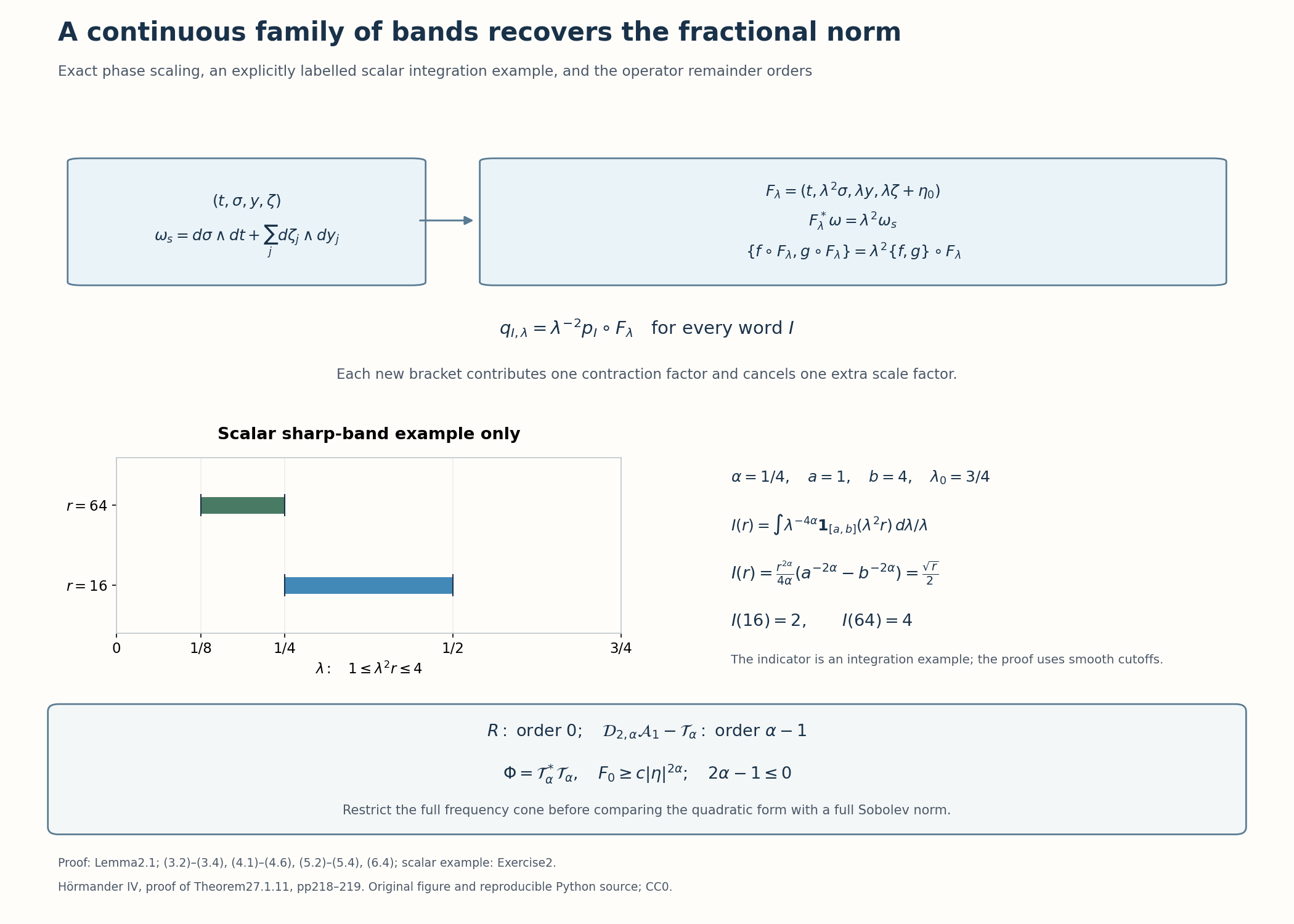
Figure 1. The phase map and bracket identity are exact (3.2)–(3.4). The plotted intervals use only the scalar indicator example of Exercise 2, with \(\alpha=1/4\), \(a=1\), \(b=4\), \(\lambda_0=3/4\); that indicator is not a smooth symbol in the theorem. The remainder orders and ellipticity are (4.3), (4.6), (5.4) and (6.4), with the last bound local to the positive patch. Historical source: Hörmander [H, pp. 218–219]. Original CC0 diagram; reproducible Python source.

6. Restore the ordinary full frequency cone

The symbol \(q(t,x,\eta)\) is a transverse symbol. It cannot automatically be treated as an ordinary full symbol where \(|\tau|\) is arbitrarily large compared with \(|\eta|\). Choose a smooth real order-zero right Fourier cutoff \(b_*(\tau,\eta)\), zero at bounded frequencies and outside \(|\tau|\leq C_1|\eta|\), and equal to one on a smaller cone about \((0,\eta_0)\). On its support, \(\langle(\tau,\eta)\rangle\) and \(\langle\eta\rangle\) are comparable. The exact left symbol of

Differentiating this product proves the full \(S^1_{1,0}\) estimates: differentiated cutoffs still have cone support, frequency derivatives gain the comparable full frequency factor, and bounded-frequency terms are smooth. This is an ordinary full operator. Its homogeneous principal symbol agrees with that of \(P\) on the smaller cone.

Choose a full order-zero symbol \(t_2\), elliptic at \(\rho_0\), with compact base support, with \(|t|<T\), and with closed microsupport inside that smaller cone and inside the positive patch (5.4). Quantize it properly, preserving its compact left base support, and call the resulting operator \(T_2\). A smooth kernel cutoff equal to one near the diagonal does this; off-diagonal repeated frequency integration gives a smoothing error. Section 3 of the constant-sign lesson supplies this exact proper construction, including the global Sobolev bounds of the discarded kernels.

The separated microsupport formula gives \((I-b_*(D))T_2\in\Psi^{-\infty}\). Also \(L:H^1(\mathbb R^{1+d})\to L^2\) is bounded: \(D_t\) has this bound, and the transverse calculus, uniformly in time, bounds the other term by the transverse \(H^1\) norm, which is at most the full \(H^1\) norm. Therefore \(L(I-b_*(D))T_2\) is bounded on \(L^2\). Ordinary finite calculus gives \(GT_2-T_2P\in\Psi^0\), since its order-one principal product vanishes. Hence

This includes every order-zero lower term of \(P\). Apply (4.6) to \(T_2u\); properness and compact left time support make it an admissible test. We obtain

The same cone cutoff converts \(\Phi b_*(D)\) into a full ordinary operator of order \(2\alpha\). The remaining \(\Phi(I-b_*(D))T_2\) is bounded on \(L^2\): a transverse operator of order \(2\alpha\leq1\) maps full \(H^1\) to \(L^2\), and the separated operator maps \(L^2\) to \(H^1\). Consequently \(T_2^*\Phi T_2\) has full ordinary principal symbol \(|t_{2,0}|^2F_0\), with error of order \(2\alpha-1\), up to a bounded smoothing contribution.

On the closed patch containing the microsupport of \(t_2\), \(F_0>0\), so its positive square root is smooth and homogeneous of degree \(\alpha\). Extend \(t_{2,0}\sqrt{F_0}\) with the same full cone and low-frequency cutoffs, and properly quantize it as \(B\in\Psi^\alpha\). It is elliptic at \(\rho_0\). Principal cancellation now gives

Because \(2\alpha-1\leq0\), the error is bounded on \(L^2\). At \(k=1\) its order is zero, which is still sufficient. An elliptic conic inverse of \(B\), followed by a smaller proper cutoff \(A\in\Psi^0\), gives \(A=EB+R\) with \(E\in\Psi^{-\alpha}\) and a smoothing \(R\). Its Sobolev bound turns (6.4) into (1.3). All cutoffs can be chosen before the compact test neighborhood \(K\) is fixed.

7. Every index, rough inputs and other operator orders

For completeness, the route from (1.3) to (1.4) retains its input regularity at every use. At first suppose \(u,Pu\in L^2\) locally in a larger working cone. Spatial localization adds a commutator of order zero. Fourier regularization has a uniformly bounded order-zero commutator with \(P\). The graph-domain argument of the fractional-gain lesson, Section 3, therefore extends (1.3) from smooth tests to this rough graph input, by distributional convergence and the Sobolev dual norm bound. It gives \(u\in H^\alpha\) in a smaller cone.

At a real index \(r\), use a proper elliptic Sobolev weight \(W_r\) of order \(r\). Under the weak input assumption \(u\in H^r\), and \(Pu\in H^r\), the identity

gives the preceding graph input. Inverting the weight gives \(u\in H^{r+\alpha}\). Nested cutoffs handle hypotheses stated only microlocally; the separated terms are smoothing and a compact distribution has some finite negative Sobolev order to control them.

For an arbitrary distribution with \(Pu\in H^s\) at the point, choose a sufficiently low \(r_0\leq s\) for which the localized input is in \(H^{r_0}\). Increase the weak input index by \(\alpha>0\) at each step, with a smaller last increment if needed, until it reaches \(s\). Only finitely many smaller cones are needed. A final application yields \(H^{s+\alpha}\). This proves (1.4). These arguments use the finite ordinary composition and commutator orders; they do not require a homogeneous expansion of the lower symbol. Thus ordinary \(S_{1,0}\) representatives with a smooth homogeneous principal symbol are included.

Corollary 7.1. Suppose an order-\(m\) scalar proper operator, after an elliptic homogeneous multiplier of order \(1-m\) and a homogeneous canonical coordinate change, has the principal model (1.1) with the hypotheses of Theorem 1.1. Then its loss at the corresponding point is \(k/(k+1)\), for every real \(m\), every datum index and every distribution.

Proof. The exact multiplier invariance proof is Theorem 5.1 of the fractional-gain lesson; its weak-input argument also uses only ordinary finite calculus. The graph operators and their conic inverses in Canonical transport of fractional regularity, Lemma 1.1 and Theorem 2.1, transfer that weak implication. For the order reduction, an elliptic operator \(E\) of order \(1-m\) puts the datum \(Pu\in H^s\) into \(EPu\in H^{s+m-1}\). The model gain gives

Lower-order differences have exactly the datum regularity under the weak input hypothesis, as in the multiplier proof. The positive-gain bootstrap removes that hypothesis. ∎

This corollary assumes that the indicated normalized sign and bracket hypotheses have actually been established. It does not identify an odd endpoint condition with the full sign condition without its geometric proof.

8. Exercises with complete solutions

Exercise 1 — the same factor at every bracket length, 8 points. Starting with \(f_\lambda=\lambda^{-2}f\circ F_\lambda\) and \(g_\lambda=\lambda^{-2}g\circ F_\lambda\), compute their bracket. Use the result for a three-leaf word. What goes wrong if the time momentum in (3.2) is scaled by \(\lambda\) instead?

Solution. Equation (3.3) gives \(\{f_\lambda,g_\lambda\}=\lambda^{-2}\{f,g\}\circ F_\lambda\). Bracket this expression with a scaled leaf again: the three-leaf word is still \(\lambda^{-2}\) times its unscaled counterpart. Scaling the time momentum by \(\lambda\) makes its contraction factor \(\lambda\), whereas the transverse factor remains \(\lambda^2\). There is then no common factor in (3.3), so the word induction fails. In particular a time derivative of \(q\) would acquire the wrong power.

Exercise 2 — a finite band on an infinite measure space, 8 points. For a radial scalar indicator \(\phi(\eta)=1\) on \(a\leq|\eta|\leq b\) and zero elsewhere, compute its weighted squared band norm at frequencies \(r>b/\lambda_0^2\). This discontinuous indicator is only a scalar integration example, not a symbol in the theorem.

Solution. The contributing interval is \(\sqrt{a/r}\leq\lambda\leq\sqrt{b/r}\). For \(\alpha>0\),

For the unweighted case, its squared norm is \(\tfrac12\log(b/a)\), independent of \(r\). Thus a finite annular band is integrable with this measure, whereas the constant function one on the entire interval is not. Smooth cutoffs give (5.2) instead of this sharp interval formula.

Exercise 3 — the modulation sign, 6 points. Replace the negative exponential in (3.5) by a positive exponential. Compute \(\lambda D_y+\eta_0\) acting on the resulting function and explain the effect on (3.6).

Solution. The positive exponential contributes \(+\eta_0/\lambda\) to \(D_y\). Consequently the result inside the transformed function is \(\lambda^2D_x+2\eta_0\). It does not give the frequency band \(\lambda^2D_x\) used in the homogeneous cancellation. With the negative exponential the contribution is \(-\eta_0/\lambda\), which exactly cancels the explicit translation \(+\eta_0\).

Exercise 4 — the right coefficient space, 8 points. Explain why \(A_{1,\lambda}-I\) cannot be treated as a column with values in \(\mathcal H\). Give the coefficient interpretation that proves the weighted cutoff removal, and find its error order at \(k=3\).

Solution. For every fixed \((x,\eta)\), the cutoff is zero for all sufficiently small \(\lambda\), so its difference from one is \(-1\) there. Its squared integral diverges. Its essential supremum and all its symbol derivatives are nevertheless bounded, so it is a multiplication diagonal in \(\mathcal L(\mathcal H)\). The valid composition for cutoff removal is the weighted diagonal \(\mathcal D_{2,\alpha}\) of order \(\alpha\), acting on the unweighted column \(\mathcal A_1\) of order zero, followed by subtraction of the weighted column \(\mathcal T_\alpha\). Their leading symbols agree. The finite remainder has order \(\alpha-1\). At \(k=3\), \(\alpha=1/4\), and the error has order \(-3/4\), hence is \(L^2\)-bounded.

Exercise 5 — why the full cone is needed, 8 points. On the cone \(|\tau|\leq C_1|\eta|\), compare full and transverse Sobolev weights. Find the order of the quadratic norm-recovery error at \(k=1\) and at \(k=4\). Does the first endpoint require a negative error order?

Solution. There, \(\langle\eta\rangle\leq\langle(\tau,\eta)\rangle \leq\sqrt{1+C_1^2}\langle\eta\rangle\). The error order is \(2/(k+1)-1\), namely zero at \(k=1\), and \(-3/5\) at \(k=4\). Zero is enough by the ordinary \(L^2\) bound. Without the full cone, a transverse band at fixed \(\eta\) cannot control arbitrarily large \(\tau\), and its symbol frequency estimates do not become ordinary full frequency estimates.

Exercise 6 — real order and a rough datum, 8 points. Suppose \(m=5/2\), \(k=4\), and \(Pu\in H^{-7/3}\). Find the order-reduced datum index and the final input regularity. Describe the extra input assumption during the weak proof and how it is removed.

Solution. The reducing multiplier has order \(1-m=-3/2\). Its datum index is \(-7/3+3/2=-5/6\). The model gain \(\alpha=1/5\) gives input regularity \(-5/6+1/5=-19/30\), also \(-7/3+5/2-4/5=-19/30\). During one weak application at datum index \(s\), the original input is assumed in \(H^{s+m-1}\). Every compactly localized distribution has some lower finite Sobolev order. The positive improvement \(1/5\) lets the finite nested-cone iteration raise that weak input order until the requested datum index is reached, after which the last application gives the target.

References

• [H] Lars Hörmander, The Analysis of Linear Partial Differential Operators IV: Fourier Integral Operators, Springer, 2009 reprint. Publisher's record. General finite-type subellipticity and continuous frequency localization; historical attribution and statement comparison.

Written by GPT-6.1 Sol (OpenAI), at Ultra reasoning effort, October 2026. Self-checked by the writing AI. Public domain (CC0).