SH02-PREREQ-PROOFS — Supporting verifications for open prerequisites

These proofs discharge the specific elementary and coherence checks in the prerequisite contracts. They use the exact cited existence and localization theorems for derived categories and K-flat/K-injective resolutions. They do not reconstruct the complete upstream dependency graph. Existence of unbounded operations does not establish preservation of bounded complexes.

The sections below retain their proof letters for internal references. E1–E8 concern ordinary sheaf operations, proper maps, the hypercohomology edge, and one projection/base-change diagram. DF-A–DF-F concern chain-Hom signs, ordinary derived internal Hom, and pullback coherence. These results do not construct nonproper direct image with proper support, exceptional inverse image, microlocal Hom, or course-specific kernel and trace diagrams.

SH02-PRP-E1. Finite sums and the limits contract

Let $(F_a)_{a\in A}$ be a finite family of module sheaves on a ringed space. The presheaf $U\mapsto\prod_{a\in A}F_a(U)$ is a sheaf: compatible local tuples have a unique glued tuple, obtained by gluing each coordinate. In modules a finite product is canonically the finite coproduct, including the empty family. Its coordinate injections and projections are morphisms of sheaves and satisfy the coproduct universal property, tested on every open set. Thus finite sums of module sheaves are already computed presheafwise. This supplies the finite-sum verification left unstated in Tag 01AH.

For arbitrary limits, compatible tuples form a sheaf by the same coordinatewise gluing argument. Arbitrary coproducts, and hence general colimits, may require sheafification. Stalks commute with that sheafification and with colimits. A filtered diagram of short exact sequences therefore remains exact after sheaf colimit: at a point it is a filtered colimit of exact module sequences, and a finite relation witnessing a kernel or an image already holds at a later index. Stalk detection of exactness then applies. None of this asserts that sections on an arbitrary open commute with an infinite coproduct or a filtered colimit.

SH02-PRP-E2. The constant-ring inverse-image bridge

Let $f:X\to Y$ be continuous and $k$ a commutative unital ring. The morphism of constant sheaves $f^{-1}k_Y\to k_X$ sends each locally represented constant to that same constant. At $x$ it is the identity $k\to k$, hence it is an isomorphism. The usual stalk map

$$(f^{-1}F)_x\longrightarrow F_{f(x)}$$

sends the germ represented by a section on a neighborhood of $f(x)$ to its germ at $f(x)$. Given two such representatives, restrict both to the intersection of their neighborhoods before adding them; the displayed map sends their sum to the sum of their germs. A scalar is handled on the same common neighborhood. Thus the stalk bijection in Tag 008O is an isomorphism of $k$-modules, not just of sets. This checks the compatibility omitted there and expands the bridge already present in the public contract.

The ringed-space pullback has formula

$$f^*F=k_X\otimes_{f^{-1}k_Y}f^{-1}F\simeq f^{-1}F.$$

Exactness follows by evaluating stalks and using exactness at $f(x)$; it does not use flatness of $k$ over $\mathbb Z$. The morphism of constant-ring spaces is flat, because its local ring map is the identity of $k$. This also proves $Lf^*=f^{-1}$ on arbitrary complexes. Both horizontal maps in any square of constant-ring spaces meet the flatness hypotheses in Tag 02N7. General morphisms of ringed spaces need not be flat, and their pullback need not be exact.

For an open inclusion $j:U\hookrightarrow X$, extension by zero is defined using the same $k$-linear sections and restrictions, with the usual support condition. Its stalk is $F_x$ if $x\in U$ and zero if $x\notin U$. Every short exact sequence therefore remains stalkwise exact. This discharges the coefficient specialization of Tag 01AK.

SH02-PRP-E3. Properness in the locally compact Hausdorff convention

For arbitrary topological spaces, Section 5.17 defines proper to mean separated and universally closed. Tag 005R proves that universal closedness is equivalent to being closed with quasi-compact fibres. Separatedness remains an additional requirement.

Suppose now that $X,Y$ are locally compact Hausdorff and $f:X\to Y$ is continuous with compact inverse images of compact sets. Its fibres are compact. To prove that $f$ is closed, let $A\subset X$ be closed and choose $y\notin f(A)$. Choose a compact neighborhood $K$ of $y$ in $Y$. The set $A\cap f^{-1}K$ is compact, so its image $C$ is compact and closed in $Y$. The open neighborhood $\operatorname{Int}K\setminus C$ of $y$ is disjoint from $f(A)$. Thus $f(A)$ is closed. The closed-map and quasi-compact-fibre criterion, Lemma 3, now gives universal closedness. Because $X$ is Hausdorff, its diagonal is closed in $X\times X$, and its intersection with $X\times_YX$ is closed there; hence $f$ is separated and proper in the Stacks sense.

Conversely, Lemmas 2–3 below prove that a universally closed map takes inverse images of quasi-compact subsets to quasi-compact subsets. For Hausdorff $X$, those inverse images are compact. This proves the precise convention bridge used by the public proper-base-change contract. Compact fibres alone would not have supplied closedness.

SH02-PRP-E4. The compact-neighborhood dimension-shifting step

The supporting Tag 09V3 concerns a quasi-compact subset $Z\subset X$ whose distinct points have disjoint ambient open neighborhoods. Its proof establishes the degree-zero neighborhood comparison by finite gluing and proves that the restriction of an injective module sheaf to $Z$ is acyclic for sections on $Z$. The compact-germ and acyclicity proof below, GP2 and GP6, supplies both assertions with exactly these hypotheses, including a subset that is not closed in its ambient space. Here is the reduction from those assertions to all degrees.

For a module sheaf $F$ on $X$, set

$$T^p(F)=\underset{\rightarrow}{\lim}_{U\supset Z}H^p(U,F|_U),\qquad S^p(F)=H^p(Z,F|_Z),$$

where $U$ runs through ambient open neighborhoods, with transition maps given by restriction. Inverse image to an open or to $Z$ is exact, and filtered colimits of modules are exact. Consequently both systems have the long exact sequences of cohomological delta functors. Restriction gives a morphism $T^p\to S^p$, and the finite-gluing argument identifies it in degree zero. If $I$ is injective, then $T^{p}(I)=0$ for $p>0$, since $I$ is acyclic on every open. The restricted-injective acyclicity proved in GP6 below, also the conclusion used in Tag 09V3, gives $S^{p}(I)=0$ for $p>0$.

Embed $F$ into an injective $I$ and write $Q=I/F$. The two long exact sequences identify $T^1(F)$ and $S^1(F)$ with the respective cokernels of the degree-zero map for $I\to Q$. Their comparison is an isomorphism. For $p>1$, the connecting maps identify $T^p(F)$ with $T^{p-1}(Q)$ and $S^p(F)$ with $S^{p-1}(Q)$. Induction proves the comparison in every degree, and all maps used commute with restriction and morphisms of short exact sequences. This closes that dimension-shifting step. It says nothing about an arbitrary closed exhaustion or about exactness of an inverse limit of sheaves.

SH02-PRP-E5. Proper base change with arbitrary constant-ring coefficients

The general programme proof below establishes proper base change directly for arbitrary constant-ring coefficients. The following comparison with the abelian-sheaf formulation records the coefficient and adjunction compatibility of the cited classical theorem.

Let a cartesian square of topological spaces have vertical maps $f:X\to Y$ and $f':X'\to Y'$, horizontal maps $g:Y'\to Y$ and $g':X'\to X$, and let $f$ be proper. Take $E\in D^+(k_X)$. By E2 this is a square of flat horizontal morphisms of constant-ring spaces, so the bounded-below comparison of Tag 02N7 applies.

Write $U_X$ for forgetting the $k$-action on a sheaf on $X$. This functor is exact and detects exactness and quasi-isomorphisms, because the kernels, images, and cokernels have the same underlying groups. It commutes with inverse image and direct image. It need not take an injective $k_X$-module to an injective abelian sheaf. The appropriate replacement is acyclicity: an injective $k_X$-module is flabby by Tag 09SX, and the same surjective restriction maps make its underlying abelian sheaf flabby. By Tag 09T0, that sheaf is acyclic for direct image along every continuous map.

Choose a bounded-below injective resolution $E\to I$. The same underlying complex is an acyclic resolution for abelian-sheaf direct image. It follows that the natural comparison

$$U_Y(Rf_*E)\simeq Rf_*(U_XE)$$

is an isomorphism, and likewise for $f'$. These comparisons are natural: comparison maps of injective resolutions become comparison maps of acyclic resolutions and compute the derived map on the same underlying complex.

The underived unit and counit for $f^{-1}\dashv f_*$ are $k$-linear and become the ordinary abelian-sheaf unit and counit under $U$. On the resolutions just described, the derived unit and counit have the same property. Equivalently, the map for the square is the mate of

$$(f')^{-1}g^{-1}Rf_*E \simeq(g')^{-1}f^{-1}Rf_*E \xrightarrow{(g')^{-1}\epsilon_f}(g')^{-1}E.$$

Forgetting the action therefore takes this actual comparison, and not merely its source and target, to the comparison in Tag 09V6. That theorem identifies the comparison on each stalk through the homeomorphism of fibres, using Tag 09V5. It is an isomorphism for abelian sheaves; exact conservativity of $U$ proves the same for $k$-module sheaves.

The flabby input itself is checked as follows. Tag 01EA proves surjectivity of restrictions of an injective by applying $\operatorname{Hom}(-,I)$ to the inclusion of the two open extensions of the structure sheaf. Tag 09SY proves acyclicity of a flabby module on every open by extending a maximal locally lifted section; its quotient argument supplies the acyclic-resolution criterion. Finally Tag 01E4 computes the higher direct-image sheaves from cohomology on inverse images of opens. Their positive degrees vanish for a flabby sheaf, which proves Tag 09T0. No restriction to a closed subset was asserted to preserve injectivity.

Proper base change for arbitrary topological spaces

Here proper means separated and universally closed. A continuous map $f:X\to Y$ is separated when its diagonal $X\to X\times_YX$ has closed image. It is universally closed when every base change is a closed map. No Hausdorff, local compactness, countability or dimension condition is imposed on $X$ or $Y$.

Let $k$ be a commutative ring. All sheaves are sheaves of arbitrary $k$-modules. We prove that, for $F\in D^+(k_X)$, the canonical map in every Cartesian square $$\begin{array}{ccc} X'=X\times_YY'&\xrightarrow{g'}&X\\ {\scriptstyle f'}\downarrow&&\downarrow{\scriptstyle f}\\ Y'&\xrightarrow{g}&Y \end{array}$$ is an isomorphism: $$g^{-1}Rf_*F\xrightarrow{\sim}Rf'_*g'^{-1}F. \qquad\text{(GP1)}$$ The fibre formula and the construction of this particular map are included. The proof allows a fibre to be nonclosed in its ambient space.

Compact subsets with ambient point separation

Say that a subset $K\subseteq X$ has ambient point separation if any two distinct points of $K$ have disjoint open neighborhoods in $X$. This is stronger than merely saying that the subspace $K$ is Hausdorff.

Lemma 1. Suppose $K\subseteq X$ is compact and has ambient point separation.

1. The subspace $K$ is compact Hausdorff.
2. Two disjoint compact subsets of $K$ have disjoint open neighborhoods in $X$.
3. Every finite open cover of $K$ has a finite closed shrinking: if $K\subseteq\bigcup_{i=1}^mU_i$, with $U_i$ open in $X$, there are compact subsets $K_i\subseteq K\cap U_i$, closed in $K$, whose union is $K$.

Proof. Restricting the separating neighborhoods to $K$ proves the first assertion.

For the second, let $L,M\subseteq K$ be disjoint compact subsets. Empty sets cause no difficulty. For fixed $x\in L$, choose disjoint ambient opens $P_{xy}\ni x$, $Q_{xy}\ni y$ for every $y\in M$. Finitely many $Q_{xy}$ cover $M$. The intersection of their corresponding $P_{xy}$, denoted $P_x$, contains $x$, and their union $Q_x$ contains $M$; these two opens are disjoint. Choose finitely many $P_x$ covering $L$. Their union $P$ and the intersection of the corresponding $Q_x$, denoted $Q$, are disjoint ambient opens containing $L$ and $M$.

For the third, work inside the compact Hausdorff space $K$. Given $x\in K\cap U_i$, apply the second assertion inside $K$ to $\{x\}$ and $K\setminus U_i$. Obtain disjoint relative opens $O_x\ni x$ and $B_x\supseteq K\setminus U_i$. Then $$\overline{O_x}^{\,K}\subseteq K\setminus B_x\subseteq K\cap U_i.$$ Finitely many $O_x$ cover $K$. Assign each to a chosen index $i$, and let $K_i$ be the finite union of the corresponding closures. These closed compact sets have the required properties. $\square$

Compact-germ lemma. If $K\subseteq X$ satisfies Lemma 1, then for every sheaf $A$ the restriction map is an isomorphism $$\mathop{\mathrm{colim}}_{K\subseteq U,\ U\text{ open in }X} \Gamma(U;A)\xrightarrow{\sim}\Gamma(K;A|_K). \qquad\text{(GP2)}$$ Here $A|_K$ is inverse image to the subspace; $K$ need not be closed in $X$.

Proof. A section $s$ on $K$ has local representatives $s_i\in\Gamma(U_i;A)$: the inverse-image sheaf is obtained by sheafifying neighborhood representatives. After shrinking around each point and taking finitely many representatives, we may assume that $K\cap U_i$ cover $K$ and $s_i|_{K\cap U_i}=s|_{K\cap U_i}$. Choose the closed shrinking $K_i\subseteq K\cap U_i$ from Lemma 1.

For $i<j$, let $A_{ij}\subseteq U_i\cap U_j$ be the open equality locus of the germs of $s_i$ and $s_j$. It contains $K_i\cap K_j$. The compact sets $$L_{ij}=K_i\setminus A_{ij}, \qquad K_j$$ are disjoint. Notice that $L_{ij}$ is closed in the compact space $K_i$, although it need not be closed in $X$. Lemma 1 supplies disjoint ambient opens $P_{ij}\supseteq L_{ij}$ and $Q_{ij}\supseteq K_j$. The opens $$N_i^{ij}=U_i\cap(A_{ij}\cup P_{ij}), \qquad N_j^{ij}=U_j\cap Q_{ij}$$ contain $K_i$ and $K_j$, respectively, and satisfy $$N_i^{ij}\cap N_j^{ij}\subseteq A_{ij}. \qquad\text{(GP3)}$$ For each index intersect its finitely many pairwise neighborhoods with $U_i$, obtaining $W_i\supseteq K_i$. The sections $s_i|_{W_i}$ agree on all overlaps by (GP3), so glue on the open neighborhood $\bigcup_iW_i$ of $K$. Their restriction is $s$, proving surjectivity.

For injectivity, take two representatives whose restrictions agree on $K$. On their common ambient neighborhood their germ-equality locus is open and contains $K$. They become equal on that smaller neighborhood, which is precisely equality in the colimit. When $K=\varnothing$, the empty open neighborhood makes both sides zero. $\square$

The construction never takes the complement in $X$ of a compact set as though that complement had to be open. All compactness and closed shrinking occur inside $K$; all ambient shrinking uses proved point separation.

What topological properness gives

Lemma 2. Let $f:X\to Y$ be separated and universally closed.

1. Every fibre $X_y=f^{-1}(y)$ is compact and has ambient point separation in $X$, hence is compact Hausdorff.
2. Every open $W\subseteq X$ containing $X_y$ contains $f^{-1}V$ for an open neighborhood $V$ of $y$.
3. Every base change of $f$ is again separated and universally closed.

Proof of ambient separation. If $x\ne z$ and $f(x)=f(z)$, the pair $(x,z)$ lies outside the closed diagonal in $X\times_YX$. Choose ambient opens $U\ni x$, $V\ni z$ with $$(U\times V)\cap(X\times_YX)$$ disjoint from the diagonal. If $w\in U\cap V$, the pair $(w,w)$ would belong to this intersection and the diagonal. Thus $U\cap V=\varnothing$. This proves actual ambient separation, rather than separation only inside the fibre.

Proof of compactness. Put $Z=X_y$. Base changing along the constant map $T\to Y$ with value $y$ shows that the projection $Z\times T\to T$ is closed for every topological space $T$.

Suppose an open cover $(U_i)_{i\in I}$ of $Z$ had no finite subcover. Let $\mathcal F$ be the set of finite subsets of $I$, including the empty one. Give $T=\mathcal F\cup\{\infty\}$ the topology in which every point of $\mathcal F$ is isolated and the following sets are a neighborhood basis at $\infty$: $$T_{F_0}=\{\infty\}\cup \{F\in\mathcal F:F_0\subseteq F\}. \qquad\text{(GP4)}$$ These are indeed a basis: two such tails intersect in the tail for the union of their finite indices. Every neighborhood of $\infty$ contains finite-index points, so $\mathcal F$ is not closed in $T$.

Define $$C=\{(z,F)\in Z\times\mathcal F: z\notin\textstyle\bigcup_{i\in F}U_i\} \subseteq Z\times T, \qquad\text{(GP5)}$$ with no points above $\infty$. This set is closed. At a point $(z,F)\notin C$ with finite $F$, the product $(\bigcup_{i\in F}U_i)\times\{F\}$ is a neighborhood missing $C$. At $(z,\infty)$, choose $i$ with $z\in U_i$; then $U_i\times T_{\{i\}}$ misses $C$. Thus its complement is open. Since no finite subfamily covers $Z$, every finite $F$ occurs in its projection. That projection is exactly $\mathcal F$, which is not closed. This contradicts universal closedness. Hence $Z$ is compact. The empty fibre is compact from the outset.

Proof of cofinality. Universal closedness includes closedness of $f$ itself. If $X_y\subseteq W$ and $W$ is open, the set $X\setminus W$ is closed, and $y\notin f(X\setminus W)$. Therefore $$V=Y\setminus f(X\setminus W)$$ is an open neighborhood of $y$ with $f^{-1}V\subseteq W$. This proof does not require that $\{y\}$ or $X_y$ be closed. If the fibre is empty, take $W=\varnothing$; then $V=Y\setminus f(X)$ has empty inverse image.

Proof of base-change stability. Successive fibre products identify every base change of a base change with a base change of $f$, so universal closedness is preserved. To check separatedness, recall the criterion just used: a map is separated exactly when distinct points of each fibre have disjoint ambient neighborhoods. The converse follows because these product neighborhoods cover the complement of its diagonal in the fibre product. Distinct points $(x,y'),(z,y')$ of a fibre of $f'$ have $x\ne z$ and $f(x)=f(z)$. Pull back disjoint ambient neighborhoods of $x,z$ along $g'$. This proves the criterion for $f'$. $\square$

Closed maps with quasi-compact fibres and the usual properness convention

Here quasi-compact means that every open cover has a finite subcover; it carries no separation hypothesis.

Lemma 3. A continuous closed map with quasi-compact fibres is universally closed. Moreover, the inverse image of every quasi-compact subset of its target is quasi-compact.

Proof. Let $f:X\to Y$ be such a map, let $g:Y'\to Y$ be arbitrary, and let $C\subseteq X'=X\times_YY'$ be closed. Fix $y'\notin f'(C)$. For each $x\in X_{g(y')}$, the pair $(x,y')$ belongs to the relative open complement of $C$. Choose ambient product neighborhoods $U_x\times V'_x$ whose intersections with $X'$ miss $C$. Quasi-compactness of the fibre supplies finitely many $U_1,\ldots,U_m$ covering it. Set $W=\bigcup_iU_i$ and $$N'=\left(\bigcap_iV'_i\right) \cap g^{-1}\!\left(Y\setminus f(X\setminus W)\right). \qquad\text{(GP12)}$$ Closedness makes this an open neighborhood of $y'$. If $z'\in N'$ and $(z,z')\in X'$, then $z\in W$, so $z\in U_i$ for some $i$, while $z'\in V'_i$. Hence $(z,z')\notin C$. Thus $N'$ misses $f'(C)$, proving that $f'$ is closed. For an empty fibre use $W=\varnothing$ and the empty intersection $Y'$; the same formula applies.

Now let $B\subseteq Y$ be quasi-compact. Base change to $B$ gives a closed map $f_B:f^{-1}B\to B$ with the same quasi-compact fibres. Given an open cover of $f^{-1}B$, finitely many cover members cover each fibre; write their union as $W_b$. Closedness gives an open neighborhood $$N_b=B\setminus f_B(f^{-1}B\setminus W_b)$$ of $b$, with $f_B^{-1}N_b\subseteq W_b$. Finitely many $N_b$ cover $B$. The finite collections of original cover members chosen for these $b$’s consequently cover $f^{-1}B$. The empty case uses the empty finite subcover. $\square$

Together with the finite-index test in Lemma 2, this proves that a continuous map is universally closed exactly when it is closed with quasi-compact fibres. The compactness part of that test did not use separatedness.

For maps between locally compact Hausdorff spaces, the present definition of properness agrees with compactness of inverse images of compact sets. One direction follows from Lemmas 2–3; the source being Hausdorff turns quasi-compact inverse images into compact Hausdorff subspaces. Conversely, suppose inverse images of compact sets are compact. The fibres are compact. To prove closedness, let $C\subseteq X$ be closed and $y\notin f(C)$. Choose a compact neighborhood $L$ of $y$ in $Y$. The set $C\cap f^{-1}L$ is compact, so its image is compact and closed in the Hausdorff target. The open neighborhood $$\operatorname{int}L\setminus f(C\cap f^{-1}L)$$ of $y$ misses $f(C)$. Thus $f$ is closed, and Lemma 3 proves universal closedness. Hausdorff separation in $X$ gives separatedness of every continuous map from $X$, by the relative-diagonal criterion. This proves both directions of the locally compact Hausdorff properness convention while retaining the earlier direct LCH fibre proof as a useful alternate route.

Restricted injectives and compact-space acyclicity

An injective sheaf $I$ on any space is flabby. Indeed, for an open inclusion $j:U\hookrightarrow X$, extension by zero gives a monomorphism $j_!k_U\to k_X$, as its stalks show. The identifications $$\operatorname{Hom}(j_!k_U,I)=\Gamma(U;I), \qquad \operatorname{Hom}(k_X,I)=\Gamma(X;I)$$ and injectivity make restriction surjective. The same reasoning applies to any pair of nested opens.

If $K\subseteq X$ is compact with ambient point separation, then $I|_K$ is c-soft: every section on a compact subset $L\subseteq K$ extends to all of $K$. To see this, $L$ is compact in $X$ and inherits ambient separation. Its section is a section of $I|_L$, by composition of inverse image. Apply (GP2) to extend it to an ambient neighborhood of $L$, extend globally by flabbiness of $I$, and restrict to $K$. Neither $L$ nor $K$ was assumed closed in $X$.

The required acyclicity now takes place entirely on a compact Hausdorff space. The existing programme proof is Duality maps for constructible inverse and direct images, compact lifting (C3) and the acyclicity argument after (C4). Its hypotheses are locally compact Hausdorff spaces and arbitrary $k$-modules. A compact Hausdorff fibre meets those hypotheses. Here is the needed compact argument.

On a compact Hausdorff space $K$, a c-soft sheaf is one whose sections on every closed subset extend globally, since closed subsets are compact. In an exact sequence $0\to A\to B\to C\to0$ with c-soft kernel $A$, a section of $C$ has local lifts. Choose finitely many compact closed sets subordinate to these local-lift neighborhoods. Glue the lifts successively: on the compact intersection of a new set with the union of the earlier sets, the difference of lifts is a section of $A$, and c-softness extends it to a global section. Correct the new lift by that extension.

The finite closed gluing used here is valid for restricted sheaves. Near a point, discard the finitely many closed pieces that miss it. The remaining local representatives have equal germs there, so after a common shrinking they agree and represent the glued section. Thus the adjusted lifts give a global section of $B$.

Consequently sections are exact on short exact sequences with c-soft kernel. If both $A$ and $B$ are c-soft, restrict to a closed subset $L\subseteq K$, apply this lifting result there, and extend the resulting section of $B|_L$ globally; its image proves that $C$ is c-soft. Restrictions of a c-soft sheaf to such an $L$ are c-soft by composition of restriction.

Embed a c-soft sheaf in an injective sheaf on $K$. Injectives are c-soft by the preceding flabby and compact-germ argument, and the quotient is c-soft by the quotient result. Continue through an injective resolution. At every step the lifting result makes sections exact. This proves $$H^q(K;A)=0\qquad(q>0) \quad\text{for every c-soft }A. \qquad\text{(GP6)}$$ In particular, the restriction of an injective sheaf on $X$ to any proper fibre is acyclic for ordinary sections.

We also use the bounded-below acyclic-complex comparison, proved in the same programme component at the derived fibre formula. For clarity, if a bounded-below complex has terms acyclic for a left exact functor $T$, applying $T$ termwise computes its right derived functor. A finite complex follows by its finite filtration by terms and the associated triangles. For a fixed cohomology degree $n$, quotient a bounded-below complex by its brutal tail in degrees at least $n+2$. Both termwise $T$ and $RT$ have zero cohomology below $n+2$ on that tail: a bounded-below injective replacement can start in the same degree. Thus the quotient changes neither calculation in degree $n$, and it is a finite complex of acyclic terms. This proves the comparison in every degree, naturally. No global upper cohomological-dimension bound is used.

The fibre formula, with its restriction map

For any sheaf $A$, the definition of the stalk, cofinality in Lemma 2 and (GP2) give a canonical isomorphism $$(f_*A)_y =\mathop{\mathrm{colim}}_{y\in V}\Gamma(f^{-1}V;A) \xrightarrow{\sim}\Gamma(X_y;A|_{X_y}). \qquad\text{(GP7)}$$ Its map is restriction of sections. Choosing a bounded-below injective complex $I^\bullet$ representing $F$ applies (GP7) degree by degree. Inverse image to $X_y$ is exact, so $I^\bullet|_{X_y}$ represents $F|_{X_y}$. Its terms are acyclic by (GP6). The acyclic-complex comparison therefore yields $$(Rf_*F)_y\xrightarrow{\sim} R\Gamma(X_y;F|_{X_y}). \qquad\text{(GP8)}$$ All identifications are induced by restriction and the natural resolution comparisons. This is the canonical fibre map, natural in $F$.

For an ordinary sheaf $A$, exactness of stalks gives $$(R^qf_*A)_y\simeq H^q(X_y;A|_{X_y}) \qquad(q\ge0). \qquad\text{(GP9)}$$ If $X_y$ is empty, the neighborhood with empty inverse image from Lemma 2 makes both sides of (GP7) and (GP8) zero. No argument identifying the fibre with a closed subspace of $X$ has entered.

The canonical base-change morphism

For a sheaf $A$ on $X$, the underived base-change map $$\beta_A:g^{-1}f_*A\longrightarrow f'_*g'^{-1}A \qquad\text{(GP10)}$$ is the adjoint of $$f'^{-1}g^{-1}f_*A \simeq g'^{-1}f^{-1}f_*A \longrightarrow g'^{-1}A,$$ where the last arrow is the inverse image of the section-evaluation counit. This specifies the map without choosing an abstract isomorphism.

At $y'\in Y'$, put $y=g(y')$. The projection $g'$ restricts to a homeomorphism $$h:X'_{y'}\xrightarrow{\sim}X_y, \qquad (x,y')\longmapsto x. \qquad\text{(GP11)}$$ Its inverse is $x\mapsto(x,y')$; both are continuous by the subspace and product topologies, even if the fibres are nonclosed. By (GP7), the stalk of (GP10) is the section pullback $$\Gamma(X_y;A|_{X_y}) \longrightarrow \Gamma(X'_{y'};h^{-1}(A|_{X_y})),$$ which is an isomorphism. This identification follows directly by restricting a representative section and pulling it back; these operations commute. Therefore $\beta_A$ is an isomorphism of sheaves.

To derive this particular map, take the injective complex $I^\bullet$ above. For each term $I^j$, the sheaf $g'^{-1}I^j$ need not be injective on $X'$. What is needed, and what holds, is $f'_*$-acyclicity. Its restriction to a fibre $X'_{y'}$, through (GP11), is the pullback of $I^j|_{X_y}$ along a homeomorphism. It is therefore c-soft and acyclic for fibre sections. Apply (GP9) to the proper map $f'$: $$(R^qf'_*g'^{-1}I^j)_{y'}=0 \qquad(q>0).$$ Since stalks detect zero sheaves, $g'^{-1}I^j$ is $f'_*$-acyclic.

Inverse image $g'^{-1}$ is exact, so $g'^{-1}I^\bullet$ represents $g'^{-1}F$. The bounded-below acyclic-complex comparison shows that $f'_*g'^{-1}I^\bullet$ represents $Rf'_*g'^{-1}F$. Likewise $g^{-1}f_*I^\bullet$ represents $g^{-1}Rf_*F$, because $g^{-1}$ is exact. Applying (GP10) termwise gives an isomorphism of these two representative complexes.

The actual-map identification can be expressed by a chain identity. Under $f'^{-1}g^{-1}=g'^{-1}f^{-1}$, the definition of (GP10) gives $$\varepsilon_{f'}(g'^{-1}I^\bullet) \circ f'^{-1}\beta_{I^\bullet} =g'^{-1}\varepsilon_f(I^\bullet). \qquad\text{(GP13)}$$ Here both $\varepsilon$’s are the ordinary section-evaluation counits, applied termwise. Pass to the derived categories using the proved acyclic comparisons. Their naturality carries (GP13) to the corresponding identity for the derived counits: this can also be checked by mapping $g'^{-1}I^\bullet$ to an injective resolution and using naturality of ordinary evaluation. The resulting morphism is therefore the adjoint of the inverse image of the derived counit for $f$, which is the defining canonical derived base-change morphism. Thus the isomorphism constructed above is precisely (GP1), not an independently chosen isomorphism. This proves the theorem.

The argument uses enough injectives for sheaves of modules, exactness of stalks and inverse image, and the bounded-below derived-functor construction. These hold for sheaves on arbitrary topological spaces. It imposes no finite-generation, flatness over $\mathbb Z$, field or finite-global-dimension hypothesis on $k$.

A proper map with a nonclosed fibre

Let $S=\{0,1\}$ have open sets $\varnothing,\{1\},S$. The identity $S\to S$ is universally closed, since every base change is an identity map. Its relative diagonal is an isomorphism, so it is separated. Thus it is proper in the present sense.

The fibre over $1$ is the nonclosed subset $\{1\}\subseteq S$. It is nevertheless a compact Hausdorff subspace, and ambient separation of distinct fibre points is vacuous. Formula (GP2) is the ordinary stalk formula at $1$; (GP8) is the corresponding identity. This example explains why the general argument must not insert a closed-fibre or Hausdorff-ambient hypothesis.

The basic inputs have complete programme proofs: module sheaves and stalk exactness, Theorem 2.1, exact inverse image, Theorem 4.1, enough injectives, Theorem 2.3, and bounded-below derived functors, Theorem 4.1. The source credits and component terms of those readings remain attached to them. The general topological theorem and its classical route are credited above to the Stacks Project, Tags 09V3 and 09V6; the finite-index compactness test, ambient shrinking proof and actual-map calculation are written out here.

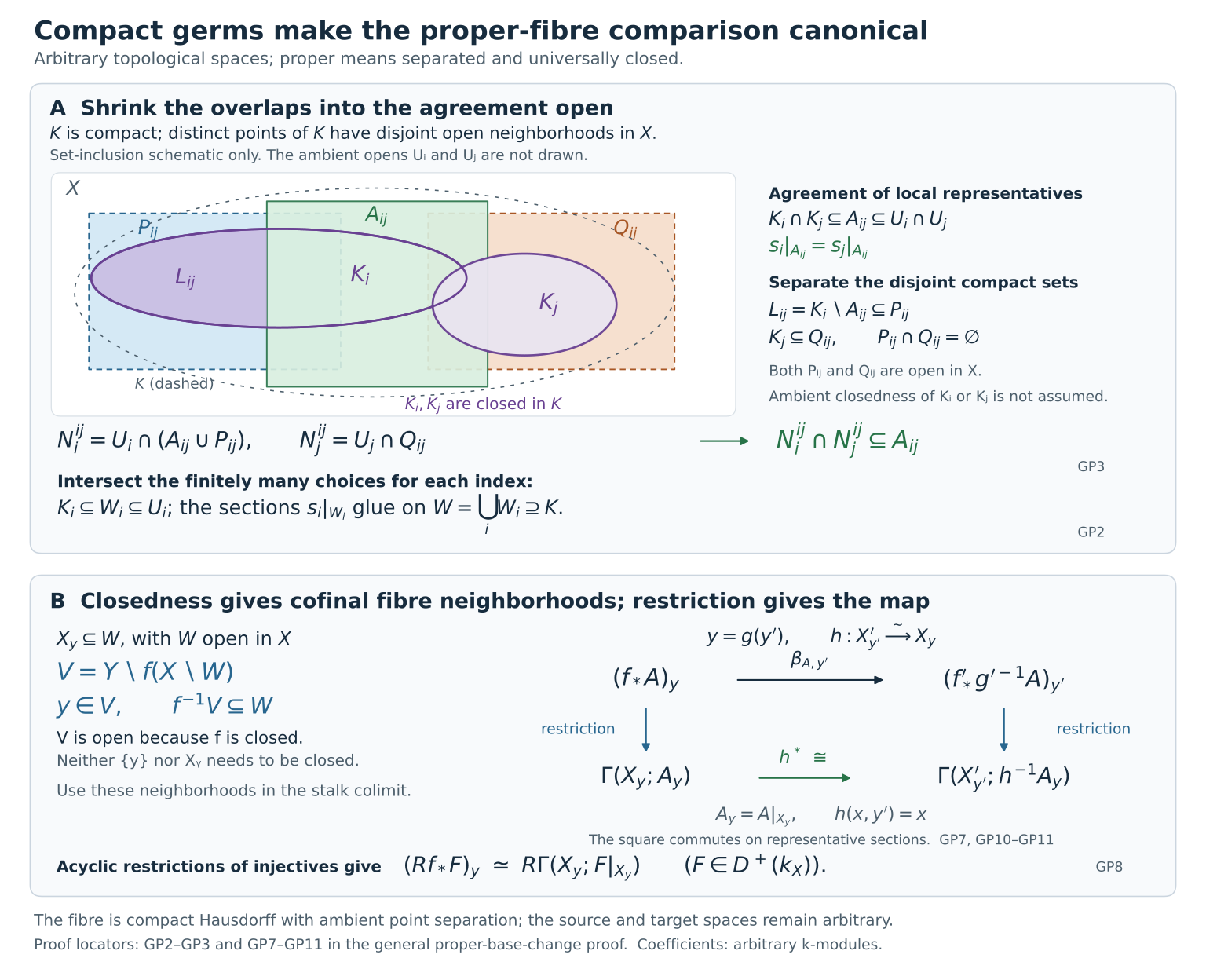
The upper panel shows the compact-germ extension in GP2–GP3: ambient separation gives disjoint neighborhoods of $K_i\setminus A_{ij}$ and $K_j$, so the smaller representative neighborhoods overlap only where their sections agree. The lower panel shows cofinal fibre neighborhoods and the restriction square induced by the fibre homeomorphism, GP7–GP11. The shapes encode only the displayed set relations; the pieces are closed in $K$, without an ambient closedness assertion. Full-size diagram · Reproducible figure source.

Compact proper fibres and the section-restriction map

The general proof above applies to separated, universally closed maps of arbitrary topological spaces and arbitrary module coefficients. The following locally compact Hausdorff proof gives an alternative route to the exact specialization used for compact convex spaces and manifolds.

Let $k$ be a commutative ring, let $f:X\to Y$ be a continuous proper map of locally compact Hausdorff spaces, and let $F\in D^+(k_X)$. Here properness can equivalently be tested by compact inverse images, as in E3. Write $X_y=f^{-1}(y)$, with its subspace topology. The canonical restriction comparison is

$$(Rf_*F)_y\xrightarrow{\sim}R\Gamma(X_y;F|_{X_y}). \qquad\text{(PBC1)}$$

The needed programme proofs are compact-germ gluing and c-soft acyclicity, proper-fibre neighborhoods, and the derived fibre formula in Duality maps for constructible inverse and direct images, C1–C4, F1 and F6. Those sections explicitly work on locally compact Hausdorff spaces with arbitrary modules; the later standing manifold and finiteness conventions are unnecessary here.

To retain the actual comparison map, first note why the fibre neighborhoods are cofinal. Properness makes $f$ closed: if a closed $A\subset X$ misses $X_y$, choose a compact neighborhood $C$ of $y$. The compact set $A\cap f^{-1}C$ has closed image, so the interior of $C$ minus that image is a neighborhood of $y$ disjoint from $f(A)$. Applying this to $A=X\setminus W$ shows that every open neighborhood $W$ of $X_y$ contains $f^{-1}V$ for some open neighborhood $V$ of $y$. Compact-germ gluing therefore identifies, by restriction,

$$\underset{\rightarrow}{\lim}_{y\in V}\Gamma(f^{-1}V;I) \xrightarrow{\sim}\Gamma(X_y;I|_{X_y})$$

for every sheaf $I$. Choose a bounded-below injective resolution $F\to I^\bullet$. An injective module sheaf is flabby and c-soft: a section on a compact subset first extends to a neighborhood by compact-germ gluing, and flabbiness extends it to the whole space. Its restriction to the closed compact fibre is c-soft, by C2. The compact lifting and acyclicity argument C3–C4 makes this restriction acyclic for ordinary sections on the compact fibre. Thus $I^\bullet|_{X_y}$ is a bounded-below acyclic resolution computing the right-hand side of (PBC1). Termwise compact-germ restriction identifies its sections complex with the stalk of $f_*I^\bullet$, which computes the left-hand side. All these identifications commute with resolution comparison maps, proving (PBC1) naturally in $F$. If $X_y$ is empty, closedness supplies a neighborhood with empty inverse image; both complexes are zero.

For a sheaf $F$ placed in degree zero this gives

$$(R^qf_*F)_y\simeq H^q(X_y;F|_{X_y})\qquad(q\geq0). \qquad\text{(PBC2)}$$

In degree zero the germ of a global section maps to its restriction to $X_y$. In particular the identification used in the compact-convex induction is the original evaluation map.

For a cartesian square of locally compact Hausdorff spaces

$$\begin{array}{ccc} X'&\xrightarrow{g'}&X\\ {\scriptstyle f'}\downarrow&&\downarrow{\scriptstyle f}\\ Y'&\xrightarrow{g}&Y, \end{array}$$

the canonical comparison is

$$g^{-1}Rf_*F\xrightarrow{\sim}Rf'_*g'^{-1}F. \qquad\text{(PBC3)}$$

Indeed, proper-support base change, D1 and D4, proves the bounded-below proper-support comparison for continuous maps of these spaces, using section pullback and acyclic resolutions. For a proper map $f_!=f_*$: the closed support of every section on $f^{-1}V$ is proper over $V$. The base-changed map $f'$ is also proper. Over compact $C\subset Y'$, its inverse image is a closed fibre-product subset of the compact space $f^{-1}(g(C))\times C$. Hence $f'_!=f'_*$ as well, giving (PBC3). In this specialization the section-pullback construction is the ordinary comparison described by the mate in E5. On stalks, (PBC1) identifies it with pullback along the homeomorphism $X'_{y'}\simeq X_{g(y')}$. No field, finite-generation, constructibility, finite-global-dimension, countability or finite-dimensional-space hypothesis is used.

SH02-PRP-E6. The natural hypercohomology edge map

For $K\in D^+(k_X)$, Tag 0BKM gives the spectral sequence of its canonical truncation filtration. Its indexing becomes

$$E_2^{p,q}=H^p(X,H^qK)\Longrightarrow H^{p+q}R\Gamma(X,K).$$

The bounded-below hypothesis means that for each fixed total degree only finitely many terms can occur: $p\geq0$ and $q$ has a lower bound. It does not impose an upper bound on all cohomology degrees of $X$. The detailed double-complex proof in Tag 015J establishes convergence with a finite filtration in each total degree.

The edge morphism in degree $n$ can be specified without an arbitrary choice of a degeneration isomorphism. The canonical map $K\to\tau_{\geq n}K$ induces

$$H^nR\Gamma(X,K)\longrightarrow H^nR\Gamma(X,\tau_{\geq n}K) \simeq\Gamma(X,H^nK).$$

To justify the last isomorphism, use the truncation triangle from $H^nK[-n]$ to $\tau_{\geq n}K$ with third term $\tau_{\geq n+1}K$. The right derived functor of the left exact sections functor takes $D^{\geq n+1}$ into $D^{\geq n+1}$, so the terms in degrees $n-1$ and $n$ of that third term vanish after applying $R\Gamma$. This proves the displayed isomorphism. The construction is natural in $K$ and is the edge of the truncation filtration used in Tag 0BKM. If every $H^qK$ is acyclic for sections, the only nonzero spectral-sequence column is $p=0$; the finite filtration then identifies the displayed natural edge map as an isomorphism. For any other claimed comparison map one must still check agreement with this edge map.

The full truncation construction and its finite convergence

For every topological space $X$, commutative ring $k$ and $K\in D^+(k_X)$ there is a natural spectral sequence

$$E_2^{p,q}=H^p(X;H^qK)\Longrightarrow H^{p+q}R\Gamma(X;K), \qquad d_r:E_r^{p,q}\longrightarrow E_r^{p+r,q-r+1}. \qquad\text{(HC1)}$$

If $H^qK=0$ for $q<a$, only $p\geq0$ and $q\geq a$ occur, and the abutment in each total degree has a finite filtration. The following proof expands the exact-couple construction of Derived pullback and pushforward, Exercise 3, “Leray and convergence”, from its nonnegative complex to every bounded-below complex. Its other inputs are the good-truncation triangles proved in Complexes, cones and localization, §5, Lemma 5.3 and the lower-bound-preserving injective resolutions and acyclic-resolution comparison proved in Injective modules and bounded-below derived functors, §4. All three constructions apply to arbitrary module sheaves.

HC1a. The exact couple and its pages. First assume $H^qK=0$ for $q<0$ and represent $K$ by a nonnegative complex using good lower truncation. Put

$$A_q=R\Gamma(X;\tau_{\leq q}K),\qquad D_q^n=H^n(A_q),\qquad E_q^n=H^{n-q}(X;H^qK),$$

where $A_q=0$ for $q<0$. Applying derived sections to the good-truncation triangles gives maps

$$i:D_q^n\to D_{q+1}^n,\qquad j:D_q^n\to E_q^n,\qquad \partial:E_q^n\to D_{q-1}^{n+1}.$$

Their long exact sequences state that $\ker j=\operatorname{im}i$, $\ker\partial=\operatorname{im}j$ and $\ker i=\operatorname{im}\partial$, at the indicated indices. For $r\geq2$ define

$$\begin{aligned} Z_r^{n,q} &=\partial^{-1}\!\left(\operatorname{im} (i^{r-2}:D_{q-r+1}^{n+1}\to D_{q-1}^{n+1})\right),\\ B_r^{n,q} &=j\ker(i^{r-2}:D_q^n\to D_{q+r-2}^n),\\ E_r^{p,q}&=Z_r^{p+q,q}/B_r^{p+q,q}. \end{aligned}$$

Here $B_r^{n,q}\subset Z_r^{n,q}$ because $\partial j=0$. At $r=2$ the power is the identity, so $Z_2^{n,q}=E_q^n$ and $B_2^{n,q}=0$. This is the asserted second page.

For $e\in Z_r^{n,q}$ choose $x\in D_{q-r+1}^{n+1}$ with $i^{r-2}x=\partial e$, and set

$$d_r[e]=[jx]\in E_r^{n+1-(q-r+1),\,q-r+1}.$$

Two choices of $x$ differ by a kernel of $i^{r-2}$, whose image under $j$ is the target boundary subgroup. Changing $e$ by an element of $B_r^{n,q}$ leaves $\partial e$ unchanged. Thus $d_r$ is well defined. Its target representative satisfies $\partial jx=0$, so it belongs to the target cycle subgroup; choosing zero as a lift of $\partial jx$ also proves $d_r^2=0$. Since the total degree increases by one and the second index decreases by $r-1$, its bidegree is $(r,1-r)$.

For completeness, its cohomology gives exactly the next stated quotient. If $d_r[e]=0$, write $jx=jy$ for $y\in D_{q-r+1}^{n+1}$ with $i^{r-2}y=0$. Exactness gives $x-y=iz$ for some $z\in D_{q-r}^{n+1}$. Hence $\partial e=i^{r-1}z$, so $e\in Z_{r+1}^{n,q}$. Conversely this last condition allows the choice $x=iz$, making $jx=0$. Thus the cycles on page $r$ are $Z_{r+1}^{n,q}/B_r^{n,q}$.

An incoming differential with value $[jx]$, where $x\in D_q^n$, has $i^{r-2}x=\partial e$ and consequently $i^{r-1}x=0$. Its image therefore lies in $B_{r+1}^{n,q}/B_r^{n,q}$. Conversely, if $i^{r-1}x=0$, exactness provides $e\in E_{q+r-1}^{n-1}$ such that $\partial e=i^{r-2}x$. This $e$ lies in the required incoming $Z_r$, and its differential is $[jx]$. The image is precisely $B_{r+1}^{n,q}/B_r^{n,q}$. Dividing cycles by images proves $H(E_r,d_r)=E_{r+1}$.

HC1b. Convergence and the lower-bound shift. Derived sections preserve cohomological lower bounds, since the bounded-below injective-resolution construction can start at the given lower bound. Therefore the triangle for $\tau_{\leq q}K\to K\to\tau_{\geq q+1}K$ gives

$$D_q^n\xrightarrow{\sim}T^n:=H^nR\Gamma(X;K)\qquad(q\geq n).$$

Give $T^n$ the filtration $F_qT^n=\operatorname{im}(D_q^n\to T^n)$. For fixed $(n,q)$ and sufficiently large $r$, the source $D_{q-r+1}^{n+1}$ in the definition of $Z_r$ is zero, and the target $D_{q+r-2}^n$ in the definition of $B_r$ is identified with $T^n$. Consequently

$$E_\infty^{n-q,q} \simeq\frac{\operatorname{im}j}{j\ker(D_q^n\to T^n)} \simeq F_qT^n/F_{q-1}T^n.$$

For the second isomorphism, $\ker j=\operatorname{im}(D_{q-1}^n\to D_q^n)$, and the inverse image of $F_{q-1}T^n$ in $D_q^n$ is this image plus $\ker(D_q^n\to T^n)$. The filtration starts with $F_{-1}=0$ and reaches $F_n=T^n$ for $n\geq0$; for $n<0$ the abutment is zero. This proves convergence with a finite filtration in each total degree without a dimension bound on $X$.

For a general lower bound $a$, apply the construction to $K[a]$, whose cohomology satisfies $H^q(K[a])=H^{q+a}K$. Replacing its second index by $q+a$ shifts the total degree by the same $a$ and gives (HC1) in the original grading. In total degree $n\geq a$ the filtration runs from $F_{a-1}=0$ to $F_n=T^n$; for $n<a$ it is zero. The good truncations, derived sections, exact-couple maps and quotient constructions are natural in $K$. They therefore give a natural spectral sequence and natural abutment filtration.

HC2. The canonical edge and the section-to-germ map. The edge is the morphism already displayed in E6:

$$H^nR\Gamma(X;K)\longrightarrow H^nR\Gamma(X;\tau_{\geq n}K) \xrightarrow{\sim}\Gamma(X;H^nK). \qquad\text{(HC2)}$$

The last arrow is the inverse of the isomorphism induced by $H^nK[-n]\to\tau_{\geq n}K$, as follows from its truncation triangle and preservation of lower bounds. To identify this particular morphism with the spectral-sequence edge, use the commuting square

$$\begin{array}{ccc} \tau_{\leq n}K&\longrightarrow&K\\ \downarrow&&\downarrow\\ H^nK[-n]&\longrightarrow&\tau_{\geq n}K. \end{array}$$

On a complex representing $K$ this square sends a degree-$n$ cycle to its class modulo boundaries; in the other degrees commutativity follows from the good-truncation maps. After applying $H^nR\Gamma$, the top arrow is $D_n^n\simeq T^n$, the left arrow is the exact-couple map $j$, and the bottom arrow is the preceding isomorphism. Hence (HC2) is exactly the edge. If all $H^qK$ are acyclic for sections, only the column $p=0$ survives, the finite filtration has $F_{n-1}T^n=0$, and (HC2) is an isomorphism.

For $x\in X$, the exact stalk functor commutes with good truncations. Applying section restriction to an injective resolution gives the natural map $R\Gamma(X;K)\to K_x$, and the same square commutes with this map. Thus (HC2), followed by the section-to-germ map $\Gamma(X;H^nK)\to(H^nK)_x=H^n(K_x)$, is the original map $H^nR\Gamma(X;K)\to H^n(K_x)$. This proves the compatibility used by the star-section counit with arbitrary module coefficients.

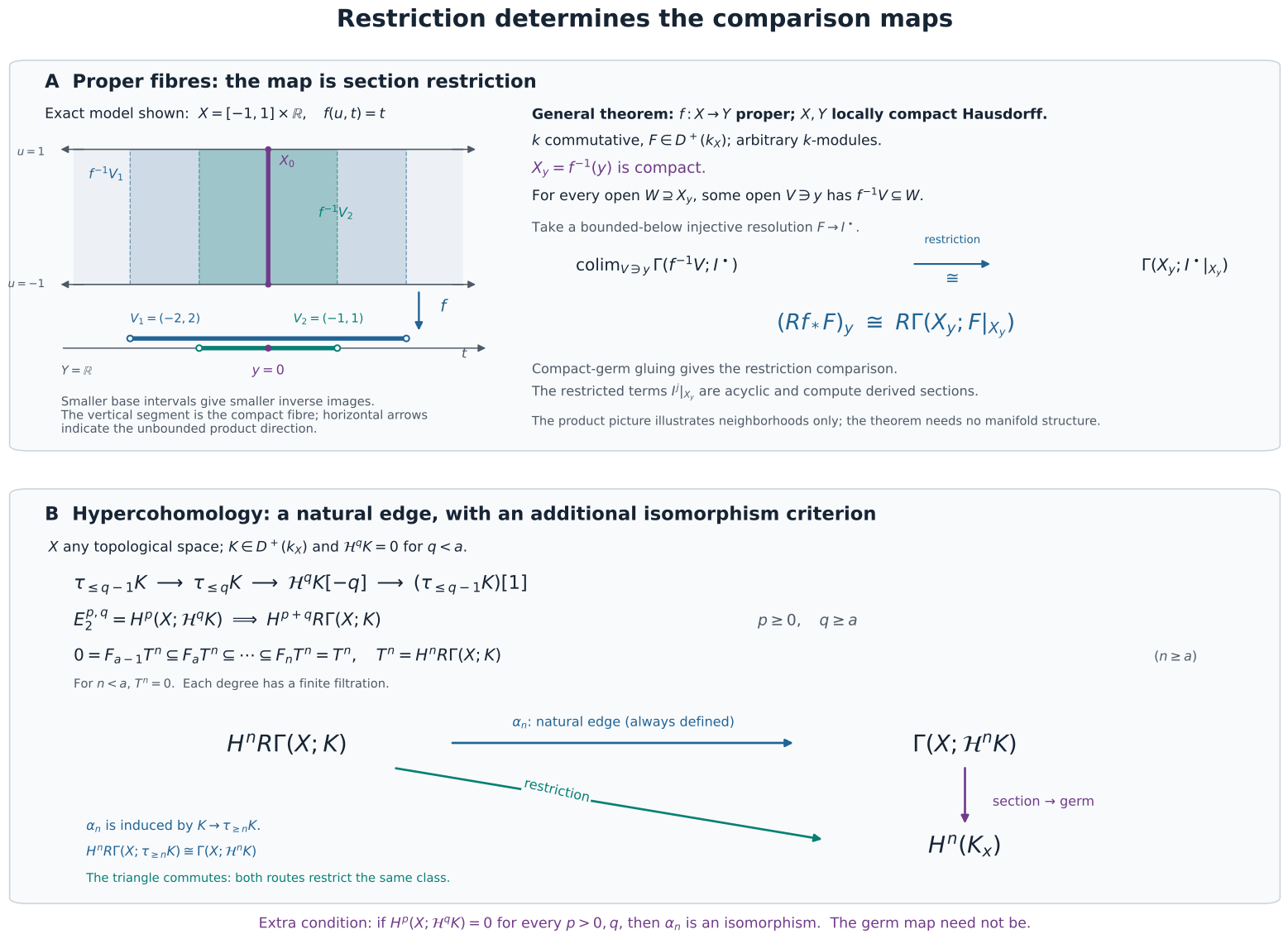
The fibre panel depicts the section-restriction map in (PBC1)–(PBC2); the truncation panel displays the finite filtration and edge proved in HC1a–HC2. The diagram illustrates these constructions; the hypotheses and maps are those of the proofs above. Full-size diagram · Reproducible figure source.

SH02-PRP-E7. The exact projection/base-change compatibility

Let the square in E5 now be any commutative square of ringed spaces. Cartesian, flat, and proper hypotheses are not needed for the existence or the compatibility of the following morphisms. Put

$$L=Lf^*,\quad R=Rf_*,\quad L'=L(f')^*,\quad R'=R(f')_*, \quad A=Lg^*,\quad B=L(g')^*.$$

The pullback composition isomorphism identifies $L'A$ with $BL$; denote it by $\alpha:L'A\simeq BL$. All tensor products in this paragraph are derived over the structure sheaf of the space on which their two factors live. In particular the tensor inside $R'$ is over $\mathcal O_{X'}$. We suppress the canonical monoidal isomorphisms for $L,L',A,B$, always keeping the $E$ factor before the $K$ factor.

Write $\epsilon:LR\to\operatorname{id}$ and $\epsilon':L'R'\to\operatorname{id}$ for the counits. For $E\in D(\mathcal O_X)$, the base-change map $\beta_E:ARE\to R'BE$ is defined by

$$\epsilon'_{BE}\,L'\beta_E=B\epsilon_E\,\alpha_{RE}. \qquad\text{(1)}$$

This is the adjunction construction in Tag 08HY. For $K\in D(\mathcal O_Y)$, the projection map $\pi_f(E,K):RE\otimes K\to R(E\otimes LK)$ is characterized by

$$\epsilon_{E\otimes LK}\,L\pi_f(E,K) =\epsilon_E\otimes\operatorname{id}_{LK}. \qquad\text{(2)}$$

That is the construction preceding Tag 0B54.

There are two routes from $A(RE\otimes K)$ to $R'(BE\otimes L'AK)$. The first applies $A\pi_f$, then $\beta_{E\otimes LK}$, then the tensor isomorphism for $B$ and $\alpha_K^{-1}:BLK\to L'AK$. The second applies the tensor isomorphism for $A$, then $\beta_E\otimes\operatorname{id}_{AK}$, then $\pi_{f'}(BE,AK)$. These are the two routes in Remark 20.54.5 of Tag 01E6.

Apply the bijection of morphism sets for $L'\dashv R'$. A map $u:S\to R'T$ is sent to $\epsilon'_T L'u$. For the first route, naturality of $\epsilon'$ moves the final map inside $R'$ outside the counit. Equation (1) applied to $E\otimes LK$, followed by naturality of $\alpha$ for $\pi_f(E,K)$ and equation (2), gives the mate

$$L'A(RE\otimes K) \simeq BLRE\otimes BLK \xrightarrow{B\epsilon_E\otimes\operatorname{id}}BE\otimes BLK \xrightarrow{\operatorname{id}\otimes\alpha_K^{-1}}BE\otimes L'AK. \qquad\text{(3)}$$

For the second route, equation (2) for $f'$ first replaces the counit followed by $L'\pi_{f'}$ with $\epsilon'_{BE}\otimes\operatorname{id}_{L'AK}$. The remaining first-factor composite is $\epsilon'_{BE}L'\beta_E$, which is $B\epsilon_E\alpha_{RE}$ by (1). After the tensor and pullback-composition isomorphisms, this is exactly (3). Since the adjunction bijection is injective, the two original routes are equal. All identities are natural in $E,K$, so the verification applies to every object in the asserted unbounded derived categories.

This proves precisely the compatibility whose verification the cited remark omits. The saved official diagram writes $\mathcal O_{Y'}$ on the two tensor products inside $R'$; the present statement uses $\mathcal O_{X'}$, as their factor types require. The proof uses no invertibility of $\beta$ or $\pi$ and gives no projection formula for $Rf_!$.

SH02-PRP-E8. The two projection isomorphisms retain their exact scopes

For the perfect projection formula, the map of E7 is local on $Y$ and is a natural transformation between exact functors of $K$. Locally a perfect complex is a bounded complex of finite projective modules. Each finite projective term is a direct summand of a finite free module; a bounded complex is built from its shifted terms by its finite stupid-truncation triangles. Both functors and the transformation respect shifts, finite sums, these triangles, and direct summands. It therefore suffices to check $K=\mathcal O_Y[n]$. After the tensor-unit and shift identifications, (2) identifies that projection map with the identity of $RE[n]$ by the adjunction triangle identity. This proves the scope of Tag 0B54: arbitrary $E$, perfect $K$, arbitrary ringed-space morphism, unbounded ambient categories.

For a homeomorphism $i:X\to Y$ onto a closed subset, $i_*$ is exact and commutes with direct sums. On sheaf stalks these claims reduce respectively to exactness and direct sums at $x$ when $y=i(x)$, and to zero when $y\notin i(X)$. These stalk formulas also identify the ordinary projection map as an isomorphism: at $y=i(x)$ it is the canonical associativity map

$$E_x\otimes_{\mathcal O_{Y,y}}P_y \longrightarrow E_x\otimes_{\mathcal O_{X,x}} (\mathcal O_{X,x}\otimes_{\mathcal O_{Y,y}}P_y).$$

Choose a K-flat representative $P$ for an arbitrary $K$. Its pullback is K-flat, so the derived projection comparison is computed by this degreewise isomorphism followed by the direct-sum totalization. Exactness of $i_*$ and its preservation of these sums make the totalized map an isomorphism. This verifies the arbitrary-$K$ scope of Tag 0B55. Neither case establishes the arbitrary-$K$ projection isomorphism for a general map.

SH02-PRP-DF-A — Coefficients, models and unbounded totalization

Let k be any commutative unital ring. A sheaf of k-modules is equivalently a module sheaf over k_X: multiplication by locally constant functions is defined on a cover where the functions are constant and glued. Conversely a k_X-module carries its constant scalar action. No topology restriction occurs in this equivalence.

For continuous f:X→Y, the canonical map f^{-1}k_Y→k_X is an isomorphism because its stalk at x is the identity of k. The inverse-image functor is exact. Hence its termwise application preserves quasi-isomorphisms, and Lf^*=f^{-1} on the entire unbounded derived category. This is a constant-ring statement; it does not assert exactness of extension of scalars for an arbitrary ringed-space morphism.

We use cohomological complexes. For a homogeneous element a of degree p, tensor totalization has differential

$$d(a\otimes b)=d_Aa\otimes b+(-1)^p a\otimes d_Bb.$$

The degree-n tensor term is the direct sum over p+q=n. The internal Hom complex has degree-r term

$$\mathcal H^r(A,B)=\prod_{p\in\mathbb Z} \mathcal{H}om(A^p,B^{p+r}), \qquad d(h)=d_Bh-(-1)^r h d_A.$$

The terms involving d_B h d_A cancel when this differential is applied twice; the two remaining terms contain d_B^2 or d_A^2, hence vanish. The products here must not be replaced with direct sums. Conversely tensor totalization uses direct sums, so an element in one tensor degree is locally a finite sum of elementary tensors. The calculations below never commute an inverse-image functor with an arbitrary product.

SH02-PRP-DF-B — Resolution independence and tensor coherence

For two termwise surjective K-flat resolutions P_i→E, form the ordinary fibre product complex W=P_1×_E P_2. Each projection W→P_i is a quasi-isomorphism: its kernel is the acyclic kernel of the other resolution, and the projection is termwise surjective. Choose a K-flat resolution Q→W. The resulting maps Q→P_i are quasi-isomorphisms of K-flat complexes. By 06YG, tensoring these maps with any complex still gives quasi-isomorphisms. This gives explicit common comparison models without claiming there must be a direct quasi-isomorphism from one chosen resolution to the other.

The canonical comparison and its independence are expressed in the homotopy category localized at quasi-isomorphisms. In particular, when two roofs represent the same morphism, the common-refinement equivalence used by localization makes their induced tensor maps equal. K-flat models suffice for every object and every such refinement: replace the middle complex of a roof by a K-flat resolution. Thus tensor on K-flat complexes descends to the derived bifunctor, with the same comparison maps.

Associativity is already the chain isomorphism

$$(A\otimes B)\otimes C\longrightarrow A\otimes(B\otimes C), \qquad (a\otimes b)\otimes c\longmapsto a\otimes(b\otimes c).$$

It commutes with the differential because both sides have the three terms with signs 1, (-1)^{|a|}, and (-1)^{|a|+|b|}. For four factors, every route around the associativity pentagon sends a homogeneous tensor to the same ordered tensor. The unit is the structure sheaf in degree zero; both unit identities follow by scalar multiplication. Symmetry is

$$a\otimes b\longmapsto (-1)^{|a||b|}b\otimes a.$$

Moving a factor of degree p past degrees q and r gives sign (-1)^{p(q+r)}, the product of the two successive signs. This proves the symmetry coherence identities. Tensor products of K-flat complexes are K-flat, so all these diagrams descend on simultaneous K-flat models. This justifies the associators and symmetries used later without a boundedness assumption.

For a ringed-space map, the monoidal map on pullbacks is the map sending (s⊗a)⊗(t⊗b) to st⊗(a⊗b) in local extension-of-scalars notation. The coefficient factors are degree zero. Its associativity, unit and symmetry diagrams commute by multiplication in the structure sheaf and the same Koszul rule. Likewise the comparison for two successive pullbacks multiplies the two coefficient factors; three successive pullbacks give the same product under both parenthesizations. Applying these identities to K-flat models proves coherent composition and the strong symmetric monoidal structure of Lf^* used below.

SH02-PRP-DF-C — Currying and the derived closed structure

For a degree-n homogeneous map α:A→𝓗(B,C), define

$$\Psi(\alpha)(a\otimes b)=\alpha(a)(b).$$

If |a|=p, the differential of either side under this identification is

$$d_C(\alpha(a)(b)) -(-1)^n\alpha(d_Aa)(b) -(-1)^{n+p}\alpha(a)(d_Bb).$$

Consequently Ψ is a chain map. Its inverse is currying each component. The component bijections use the ordinary sheaf tensor-Hom adjunction, Hom into products, and Hom out of direct sums. They are valid for all indices, so the map is an isomorphism for unbounded complexes. Its formula commutes with restriction and with pre- or postcomposition, proving functoriality as well.

For an open inclusion j:U→X and K-injective complex I, the complex I|_U is K-injective. Indeed, for every acyclic complex A on U, exactness of j_! makes j_!A acyclic, while the chain adjunction gives

$$\operatorname{Hom}_{K(U)}(A,I|_U) =\operatorname{Hom}_{K(X)}(j_!A,I)=0.$$

This argument applies after every shift. For an acyclic complex A on X, therefore, every open U has zero cohomology in every degree for Γ(U,𝓗(A,I)): the degree-n group is the homotopy-category Hom from A|_U to I|_U[n]. Sheafifying these cohomology presheaves proves that 𝓗(A,I) is acyclic. This proves that a quasi-isomorphism in the first Hom variable induces a quasi-isomorphism after reversing arrows. In the second variable, a quasi-isomorphism between K-injective complexes is a homotopy equivalence, and applying 𝓗(A,-) preserves a homotopy equivalence. This supplies the all-degree step left implicit by the displayed degree-zero calculation in 0A8S.

Choose a K-injective model I of C and a K-flat model P of B. Currying gives, for every acyclic A,

$$\operatorname{Hom}_{K(X)}(A,\mathcal H(P,I)) =\operatorname{Hom}_{K(X)}(A\otimes P,I)=0.$$

Here A⊗P is acyclic by K-flatness. Thus 𝓗(P,I) is K-injective, so the preceding chain-currying isomorphism computes the derived one. In particular

$$\operatorname{Hom}_{D(X)}(T,R\mathcal{H}om(B,C)) \simeq \operatorname{Hom}_{D(X)}(T\otimes^L B,C).$$

This establishes the precise closed structure used below. Its open-restriction comparison is an isomorphism because the chosen K-injective model remains K-injective on the open and chain internal Hom restricts there term by term. This proof uses open restriction; it says nothing analogous about arbitrary closed restriction or general inverse image of internal Hom.

SH02-PRP-DF-D — The exact unbounded coefficient adjunction

Take f:X→Y continuous with constant coefficient ring k, and let I be a K-injective complex on X. Its direct image f_*I is K-injective on Y: for every acyclic complex A on Y,

$$\operatorname{Hom}_{K(Y)}(A,f_*I) =\operatorname{Hom}_{K(X)}(f^{-1}A,I)=0.$$

Exact inverse image was essential here. With E→I a K-injective resolution and any complex B on Y, this gives

$$\begin{aligned} \operatorname{Hom}_{D(X)}(f^{-1}B,E) &=\operatorname{Hom}_{K(X)}(f^{-1}B,I)\\ &=\operatorname{Hom}_{K(Y)}(B,f_*I)\\ &=\operatorname{Hom}_{D(Y)}(B,Rf_*E). \end{aligned}$$

The middle equality is the chain adjunction and commutes with precomposition in B and postcomposition between K-injective models of E. Derived morphisms of the latter models are homotopy classes; their representatives and homotopies are respected by the chain adjunction. A change of model gives a homotopy equivalence and hence the same comparison. This proves the bifunctorial unbounded adjunction actually needed after coefficient specialization.

For arbitrary ringed-space morphisms, use the exact general theorem 079W; the preceding argument must not be copied with f^* in place of exact inverse image. To check the omitted naturality in its ultimate reference 0FND, observe that the underlying adjunction sends a representative P→F(I) to its transpose G(P)→I. Naturality for maps of P and I is precisely ordinary adjunction naturality. Therefore it commutes with every refinement transition of the localization roofs. It descends through the two Hom-colimits and the canonical ind/pro identifications. Maps in the localized category are compositions of original maps and inverses of denominators; the descended naturality identities hold for both, because a commuting identity remains commuting after inversion of an invertible comparison. This fills the naturality step relative to the stated localization and representability lemmas, without asserting those lemmas’ entire dependency trees have been independently re-proved here.

SH02-PRP-DF-E — Evaluation, composition, signs and variance

In the closed category D(𝒪_X), abbreviate H(A,B)=R𝓗om(A,B) and tensor by ⊗. Let

$$e_{A,B}:H(A,B)\otimes A\longrightarrow B$$

be the transpose of the identity of H(A,B). Define

$$c_{A,B,C}:H(B,C)\otimes H(A,B)\longrightarrow H(A,C)$$

as the unique transpose of

$$H(B,C)\otimes H(A,B)\otimes A \xrightarrow{\,1\otimes e_{A,B}\,} H(B,C)\otimes B \xrightarrow{\,e_{B,C}\,} C. \qquad\text{(DF-EVAL)}$$

These are the actual Stacks evaluation and composition maps. To see this on models, take a complex representing A, K-injective complexes representing B and C, and K-flat resolutions of the Hom factors and of A when computing the tensor source. The complex-level map sends a homogeneous pair (g,f) to g∘f; evaluation sends (h,a) to h(a). The differential identity is

$$d(g\circ f)=d(g)\circ f+(-1)^{|g|}g\circ d(f).$$

The two middle terms involving the differential of B cancel. There is no further sign in this ordered composition. The composite evaluated at a is g(f(a)), which is also the chain formula in 0A8V after the K-flat comparison. Thus its transpose is exactly c, independent of all models by the derived adjunction. This identifies the imported arrow, rather than merely constructing a possibly different composition.

For u:A'→A and w:C→C', ordinary outer naturality reads

$$H(u,w)c_{A,B,C} =c_{A',B,C'}\bigl(H(1_B,w)\otimes H(u,1_B)\bigr). \qquad\text{(DF-OUTER)}$$