Covector tests of normal limits

Independently expressed programme text is dedicated under CC0 1.0 Universal. This lesson constructs microlocalization, its directional tests, recovery maps and operation comparisons. The source account below compares these arguments with Kashiwara and Schapira, Microlocal Study of Sheaves, Astérisque 128 (1985), and identifies the separate orientation and adjunction calculations used here. The exact identification of the two transformed vertical arrows is proved in Following the microlocal comparison maps, SH02-MEP-SUPPORT and SH02-MEP-TRACE. The stated prerequisite boundaries remain part of the mathematical claims.

SH02-MIC-SOURCES — Tests, recovery maps and operation squares

The classical construction is compared with Kashiwara and Schapira, Microlocal Study of Sheaves, Astérisque 128 (1985), §§2.2–2.3, printed pp. 43–48. Definition 2.3.1 takes the Fourier–Sato transform of specialization. Proposition 2.3.2 gives the conic object, its two zero-section recoveries, its stalk and convex-cone tests; Corollary 2.3.3 gives the boundary triangle. The source obtains these from specialization and Fourier formulas. The present text follows that mechanism, with the negative closed pairing cut written as a tensor kernel and positive deformation parameter fixed throughout. Its bounded arbitrary-module setting uses the finite-dimensional manifold and coefficient hypotheses stated below; the source’s bounded-below statements are not a substitute for those amplitude proofs.

SH02-MIC-OPEN-TESTS makes the base of each test part of its condition: a cone over an open base is tested in the restricted normal bundle, while the supporting set is closed in the ambient manifold. The stalk argument treats strict positivity away from the zero section, compact unit directions and the zero-covector case separately. The supported-cone argument keeps the orientation line inside supported cohomology before using its self-duality, and uses interior in the total normal bundle. These details specify how the classical test formulas are used; the normal-cone neighborhood and Fourier section theorems remain named prerequisites.

The recovery proof REC1–REC20 is a map calculation beyond the object identifications in Proposition 2.3.2. It compares the original exceptional-inverse Fourier exchange with the raw supported-section Hom map, using the full paired adjunction identities. REC8 measures their parity and REC16 normalizes compact recovery. REC18–REC20 then identify support forgetting with the right-ordered relative trace and transport the connecting arrow of the entire triangle. The rank-one test detects the sign but does not prove the general map identity. Neither that exact parity recipe nor the course’s raw unit and counit normalizations are attributed to the source. The diagram below depicts this programme calculation.

For operations, Propositions 2.2.2–2.2.3 construct the specialization comparisons and their trace square by deformation-space base change; Propositions 2.3.4–2.3.5, p. 48, apply Fourier exchange to obtain the direct comparison and inverse-image square. The source’s Fourier section §2.1, including Propositions 2.1.5–2.1.6 on p. 41, records those exchanges without proofs. Here the normal derivative is factored into a bundle map and a base change, all four orientation-corrected endpoints are kept, and their actual adjunction mates are supplied by the named Fourier and endpoint proofs. The proper-direct result retains each support-properness condition; transversality only supplies the normal geometric condition. The inverse result distinguishes a normal-bundle isomorphism from the stronger submersion conditions that make the full comparison an isomorphism.

The order here is directional tests, map-normalized recovery, the two functorial squares, adjunction compatibility, and tensor operations. It reorganizes and expands the classical construction, with additional explicit endpoint and sign calculations. The external tensor comparison requires independent conicity, and the internal comparison uses the diagonal and its positive-transpose addition map; neither is promoted to an unconditional isomorphism. The five solved problems retain the same mathematical scope as the body. Human mathematical antecedents are credited without copying or relicensing their expression.

SH02-MIC-SETUP — Normal and conormal variables

Fix a commutative ring $k$ of finite global dimension. All manifolds are finite dimensional, Hausdorff, and countable at infinity. Maps and submanifolds are $C^\infty$; the real analytic setting is included. In the sheaf-operation statements below, a smooth map means a submersion, not merely a $C^\infty$ map. We work with bounded complexes of arbitrary sheaves of $k$-modules. Neither constructibility nor finite generation, perfectness, a field of coefficients, compactness, or orientability is assumed.

Let $i:M\hookrightarrow X$ be a closed embedded submanifold of codimension $c$. For a locally closed submanifold, restrict first to an open ambient neighborhood in which it is closed; restriction compatibility makes the construction independent of that neighborhood. Set $$E=N_MX=TX|_M/TM,\qquad E^*=N_M^*X, \qquad \tau:E\to M,\quad \pi:E^*\to M.$$ Write $e:M\hookrightarrow E$ and $s:M\hookrightarrow E^*$ for zero sections. A dot removes the zero section; thus $\dot\pi:\dot E^*\to M$. If a map to $X$ is intended, it is explicitly $i\pi$.

For a map $f:Y\to X$, the invertible relative orientation complex is $$\omega_f=\omega_Y\otimes f^{-1}\omega_X^{\otimes-1}, \qquad \omega_X=\operatorname{or}_X[\dim X].$$ In particular $\omega_i=\operatorname{or}_{M/X}[-c]$. The unshifted line $\operatorname{or}_{M/X}$ is the orientation line of the normal bundle, with its self-duality supplied by the sign representation. Tensor products are derived. Orientation evaluation and the Koszul symmetry of shifted factors are part of every displayed cancellation.

The following contracts are needed, at the stated generality.

The labels in this table are local dependency aliases; unresolved aliases remain explicit dependencies. No unbounded version is asserted.

SH02-MIC-DEFINITION — The transform after specialization

The normal specialization $\nu_MF$ is the positive deformation limit on $E$. For $p:E\times_M E^*\to E$, $q:E\times_M E^*\to E^*$, use the Fourier convention $$T_EA=Rq_!\bigl(p^{-1}A\otimes k_{\{\langle v,\xi\rangle\leq0\}}\bigr).$$ The tensor factor is extension of the constant sheaf from the indicated closed set. It is not the functor of sections with support. Define $$\mu_MF=T_E\nu_MF. \qquad\text{(MIC1)}$$ Bounded specialization is conic; the Fourier functor preserves conicity and has finite cohomological amplitude in fixed finite rank. Consequently $$\mu_M:D^b(k_X)\longrightarrow D^b_{\mathbb R_{>0}}(k_{E^*})$$ is well defined. These amplitude bounds use the manifold and coefficient hypotheses in the prerequisite contracts. Fibrewise conicity includes the zero section and does not mean that nonzero directions determine the object at zero.

SH02-MIC-OPEN-TESTS — Testing an open set of covectors

If $V\subset E^*$ is open and fibrewise convex conic, put $B=\pi(V)$. The polar is $$V^\circ=\{v\in E|_B:\langle v,\xi\rangle\geq0 \text{ for every }\xi\in V_{\tau(v)}\}.$$ It is closed in $E|_B$, and need not be closed in $E$. Empty fibres outside $B$ are excluded from this definition. For every integer $r$, $$H^r(V;\mu_MF) \simeq\underset{\rightarrow}{\lim}_{U,Z}H^r_{Z\cap U}(U;F), \qquad\text{(MIC2)}$$ where $U\subset X$ is open with $U\cap M=B$, $Z\subset X$ is closed, and $$C_M(Z)|_B\subset V^\circ. \qquad\text{(MIC3)}$$ Equivalently one may work in any open ambient neighborhood whose intersection with $M$ is $B$, and take closed supports in that neighborhood. The condition is relative to $B$; it does not prohibit support outside that base. Neighborhood restriction and enlargement of support supply the transition maps. Intersections of neighborhoods and unions of finitely many supports give common refinements, because the normal cone of a finite union is the union of its normal cones.

Proof. Fourier testing on an open convex cone gives $$R\Gamma(V;T_E\nu_MF) \simeq R\Gamma_{V^\circ}(E|_B;\nu_MF|_{E|_B}).$$ Choose an open $O\subset X$ with $O\cap M=B$; such an $O$ exists because $B$ is open in $M$. Specialization is local in the ambient space, so the last complex uses specialization of $F|_O$ along $B$. The closed-conic support formula for specialization, applied in $O$, identifies its degree $r$ cohomology with the colimit of $H^r_{Z'\cap U}(U;F)$ over neighborhoods $U$ of $B$ in $O$ and closed $Z'\subset O$ with $C_B(Z')\subset V^\circ$.

A support $Z'$ closed in $O$ is the intersection with $O$ of its closure $Z$ in $X$. At every point of $B$, both sets have the same germ; therefore their normal cones over $B$ agree. Conversely a closed $Z\subset X$ satisfying MIC3 restricts to an allowable support in $O$. Any $U$ with $U\cap M=B$ has a common refinement with $O$, namely $U\cap O$. These two observations identify the indexing systems, with the same restriction and support morphisms. Filtered colimits of modules are exact, so the degreewise specialization formula yields MIC2. This argument also proves independence of $O$. $\square$

The base qualification is essential. If $X=M=\mathbb R$, $F=k_X$, and $V=(0,1)$ in the rank-zero conormal bundle, MIC2 is $H^0((0,1);k)=k$. Imposing instead the global condition $C_M(Z)\subset V$ forces a globally closed $Z\subset(0,1)$. A constant section on the connected interval supported on such a proper subset must vanish, so every corresponding $H^0_Z((0,1);k)$ is zero. This demonstrates why the local-base interpretation cannot be omitted.

SH02-MIC-STALKS — One covector and strict positivity

For $p\in E^*$, let $x=\pi(p)$. Then $$H^r(\mu_MF)_p \simeq\underset{\rightarrow}{\lim}_Z H^r(R\Gamma_ZF)_x, \qquad C_M(Z)_x\subset\{v:\langle v,p\rangle>0\}\cup\{0\}, \qquad\text{(MIC4)}$$ where closed supports are taken locally near $x$, or extended by closure to $X$.

Proof. Open convex conic neighborhoods are cofinal for computing stalks of a conic complex. For a nonzero $p$, choose convex angular neighborhoods and saturate by positive scaling; interval contraction identifies their derived sections with those of sufficiently small ordinary convex neighborhoods. At zero, a conic open neighborhood contains the entire fibre over a sufficiently small base neighborhood, and radial contraction gives the same statement. Thus take the colimit of MIC2 over these $V$.

Suppose $C_M(Z)|_{\pi(V)}\subset V^\circ$ and $p\in V$. If a nonzero $v\in C_M(Z)_x$ had $\langle v,p\rangle=0$, a sufficiently small perturbation of $p$ in $V_x$ would pair negatively with $v$. This is impossible. Hence every such support satisfies the strict condition in MIC4.

Conversely assume that strict condition. Trivialize $E$ near $x$, choose a fibre norm, and intersect the closed cone $C_M(Z)$ with the unit-sphere bundle. Its fibre at $x$ is compact. If nonempty, the pairing with $p$ has a positive minimum on it. Compactness and closedness imply that this lower bound, weakened by a factor of two, persists for covectors in a neighborhood of $p$ and cone directions over a sufficiently small base neighborhood. Indeed a contrary sequence has a convergent unit-direction subsequence producing a forbidden direction over $x$. If the unit fibre is empty, properness of the local sphere projection shows that it stays empty after shrinking the base. In either case choose a convex conic neighborhood $V$ of $p$ small enough that all these pairings are nonnegative. Then MIC3 holds over its base. This proves cofinality of the supports. The remaining neighborhood colimit in MIC2 is exactly the stalk of $R\Gamma_ZF$; taking cohomology commutes with these filtered colimits. $\square$

At $p=0$, strict positivity allows only $C_M(Z)_x\subset\{0\}$. This case is included in the compactness argument; it is not obtained by dividing by $\|p\|$.

SH02-MIC-CLOSED-TESTS — Supports in a proper cone

Let $D\subset E^*$ be closed, fibrewise convex and conic, contain the whole zero section, and contain no line in any fibre. Let $a(v)=-v$. For every $r$, $$H_D^r(E^*;\mu_MF\otimes\pi^{-1}\operatorname{or}_{M/X}) \simeq\underset{\rightarrow}{\lim}_U H^{r-c}(U;F), \qquad\text{(MIC5)}$$ where $U\subset X$ is open and $$C_M(X\setminus U)\cap\operatorname{Int}((D^\circ)^a)=\varnothing.$$ Interior means interior in the total normal bundle. It cannot be replaced without proof by a fibrewise interior when the cone changes with the base.

Proof. The supported Fourier formula applied to $A=\nu_MF$ is $$R\Gamma_D(E^*;T_EA) \simeq R\Gamma(\operatorname{Int}((D^\circ)^a); A\otimes\tau^{-1}\operatorname{or}_{M/X})[-c].$$ Replace the Fourier input $A$ by $A\otimes\tau^{-1}\operatorname{or}_{M/X}$. The projection formula moves this locally free rank-one line to the corresponding line on $E^*$, exactly as on the left of MIC5. Its second copy on the right cancels the displayed line, using the fixed self-duality. The result is $R\Gamma(\operatorname{Int}((D^\circ)^a);\nu_MF)[-c]$. Apply the open-conic neighborhood formula for specialization and take degree $r$. The shift changes the degree to $r-c$. The orientation line remains inside sections until this cancellation; it is not a fixed global coefficient module on a nonorientable bundle. $\square$

SH02-MIC-ZERO — Two recoveries and their boundary triangle

There are natural isomorphisms $$s^{-1}\mu_MF\simeq R\pi_*\mu_MF\simeq i^!F, \qquad s^!\mu_MF\simeq R\pi_!\mu_MF \simeq i^{-1}F\otimes\omega_i. \qquad\text{(MIC6)}$$ The ordinary recovery is the no-cut Fourier base change followed by the specified specialization counit. For the compact recovery, use $(-1)^c$ times the specific zero-cone FS14 recovery, followed by the inverse specialization restriction unit. This normalization is part of MIC6. The proof below shows that original R4 has exactly this normalization; the unmodified FS14 map has the codimension-parity discrepancy REC8.

For $j:\dot E^*\hookrightarrow E^*$, the resulting distinguished triangle is $$i^{-1}F\otimes\omega_i \xrightarrow{\theta_i(F)\sigma_{i^{-1}F,\omega_i}}i^!F \longrightarrow R\dot\pi_*(j^{-1}\mu_MF)\xrightarrow{+1}. \qquad\text{(MIC7)}$$ All three arrows are transported from the zero-section localization triangle by the selected recoveries. In particular the displayed first arrow is the right-ordered relative trace, and the last arrow uses the same first-term normalization.

Proof. We specify and compare the maps in six steps.

Objects and exact suppliers.

Let the coefficient ring be commutative, unital, and of finite global dimension. Let the manifolds be finite dimensional, Hausdorff, and countable at infinity. Let $i:M\hookrightarrow X$ be a closed smooth embedded submanifold of codimension $c$, and let $F\in D^b(k_X)$ be arbitrary. The locally closed case is obtained by first restricting to an ambient open set in which the submanifold is closed. All maps constructed below commute with those restrictions.

Put $E=N_MX$, with projection $\tau$ and zero section $e$, and put $E^*=N_M^*X$, with projection $\pi$ and zero section $s$. Write $$A=\nu_MF,\qquad H=T_EA=\mu_MF,\qquad W=\operatorname{or}_{E}[c],\qquad \Omega=\omega_e\simeq\omega_i,\qquad \varepsilon=(-1)^c. \qquad\text{(REC1)}$$ The line $\Omega$ is identified with the inverse of $W$ by the specific counit-normalized map $$d:\Omega\otimes W\longrightarrow k_M \qquad\text{(REC2)}$$ of FF3a. The comparison $\omega_e\simeq\omega_i$ is MEP5/O13, with positive time direction, tangent directions before normal directions, and every shifted-line symmetry retained. A tensor permutation below means the Koszul symmetry, not an unsigned permutation.

No field, finite-stalk, constructibility, orientability, compactness, noncharacteristic, or properness condition on an input is imposed. All amplitudes are the bounded microlocalization amplitudes already required for $A,H$. The intermediate linear calculation holds on conic $D^+$ with a single global lower bound over a locally compact Hausdorff base, in finite bundle rank. Locally constant ranks may be treated componentwise only with the same required global bounds.

The exact cut consists of SH02-SP-ZERO, SH02-SP-DIRECT, SH02-SP-INVERSE, SH02-SP-ADJUNCTION and the rank-zero specialization identification; conic ordinary and proper contraction with their support counits; FS2 and the zero-cone instance of FS14; FF3a, FF4 and the original R2/R4 of FF8; LFT30 and the already proved full natural-transformation equations LFT-P0/P2; MEP5, O13/O14 and MEP14; and the six-operation base-change, projection-formula, module, adjunction and transitivity maps used by those suppliers.

The actual endpoints on the normal zero section.

Let $$u_F:i^{-1}F\longrightarrow e^{-1}A, \qquad c_F:e^!A\longrightarrow i^!F \qquad\text{(REC3)}$$ be exactly the restriction unit and boundary/counit maps proved invertible in SH02-SP-ZERO. Consider the map of pairs $i:(M,M)\to(X,M)$. Its normal map is $e:0_M\to E$; specialization along the whole source is the identity, using the positive-interval identification. The two inverse specialization comparisons become $$\alpha_F:e^{-1}A\longrightarrow i^{-1}F, \qquad \beta_F:i^!F\longrightarrow e^!A.$$ Then $$\alpha_F=u_F^{-1},\qquad \beta_F=c_F^{-1}. \qquad\text{(REC4)}$$

For the first identity, substitute the positive-square ordinary base-change definition of $\alpha$. Precomposing by the restricted unit defining $u_F$ gives the restriction unit for the rank-zero deformation $M\times\mathbb R$. Its further positive-interval restriction and contraction is the identity. This is naturality of the ordinary unit followed by the unit/counit triangle; it proves $\alpha_Fu_F=1$. Since $u_F$ is invertible, it proves the assertion with the specified map.

For the second identity use the exact exceptional-mate formula SH02-SP-SHRIEK-MATE. At this map of pairs the proper direct comparison is $e_*L\to\nu_Mi_*L$. The zero-normal axis in the deformation is a closed embedding, hence proper. On that axis the comparison is base change for this closed embedding followed by the restriction counit for the positive interval. Its central restriction is therefore the canonical identification $e_*L\simeq\nu_Mi_*L$ used in the proof of SH02-SP-ZERO; the endpoint class and positive time shift cancel there with coefficient one. Taking its $e_*\dashv e^!$ mate and composing with the specialized support counit gives exactly the map denoted $\sigma$ at the end of that proof. That proof established $c_F\sigma=1$ by reducing naturally to $F=i_*L$. Thus $\beta_F=\sigma=c_F^{-1}$. This uses neither a purity assertion for arbitrary $F$ nor a choice of a new orientation map.

Original R2 is the ordinary recovery inverse.

Temporarily let $A$ be any conic input in the linear domain. Denote the contraction maps by $$k_\tau^!:e^!A\longrightarrow R\tau_!A, \qquad k_\pi^*:R\pi_*T_EA\longrightarrow s^{-1}T_EA.$$ Let $z_A:s^{-1}T_EA\to R\tau_!A$ be proper base change at the zero covector. The cut $\langle x,0\rangle\leq0$ is the whole normal bundle, so this is the actual no-cut base-change map. If $E_e$ denotes original R2, then $$z_A k_\pi^*E_e(A)=k_\tau^!. \qquad\text{(REC5)}$$

Indeed, R2 is the right mate of the primitive kernel map $A_e:\pi^{-1}L\to T_Ee_*L$. Its ordinary adjunct at $A$ is $$\pi^{-1}e^!A\xrightarrow{A_e}T_Ee_*e^!A \xrightarrow{T_E(\epsilon_e)}T_EA.$$ Restrict to $s$ and apply $z_A$. Kernel base-change pasting turns this into $R\tau_!$ of $e_*e^!A\to A$, which is precisely $k_\tau^!$. The equality of adjuncts proves REC5. Consequently the ordinary MIC6 recovery is exactly $$r_F^*=c_FE_e(A)^{-1}:R\pi_*H\longrightarrow i^!F. \qquad\text{(REC6)}$$

The original R4 and the FS14 choice.

Let $$Z_A:R\pi_!T_EA\longrightarrow e^{-1}A\otimes\Omega \qquad\text{(REC7)}$$ mean the compact recovery obtained by the specific zero-cone FS14 proof: apply the fully faithful inverse of the raw FS2 adjunction to derived Hom, use the zero-section test coefficient, then conic contraction. This specifies a map, not just an object isomorphism.

Let $D_e:T_0(\Omega\otimes e^{-1}A)\to R\pi_!T_EA$ be original R4. Since $T_0=1$, its source is $\Omega\otimes e^{-1}A$. The exact relation is $$Z_AD_e(A)=\varepsilon\,\sigma_{\Omega,e^{-1}A}. \qquad\text{(REC8)}$$

Here is the complete map calculation. Use the already fixed linear notation $$P=T_{E^*},\quad M=a_{E^*}^{-1}(-)\otimes W, \quad V=MT_E,\quad Q=V_{E^*}.$$ Let $v:PV\to1$ be the counit of $P\dashv V$, let $\alpha:1\to PV$ be the transported unit of $V\dashv P$, and let $b:PM\to Q$ be the actual input-antipode exchange LFT-P1. The full, already proved equations LFT-P0/P2 are $$v\alpha=\varepsilon\,1,\qquad b_{T_E}\alpha=\eta, \qquad\text{(REC9)}$$ where $\eta:1\to QT_E$ is the raw FS2 unit in the specified inverse presentation. In particular $b_{T_E}v^{-1}=\varepsilon\eta$. This equation holds on every conic input; the present proof does not extrapolate it from a scalar test.

For an output $K$, let $$J_K:e^{-1}QK\xrightarrow{\sim}R\pi_!K\otimes W \qquad\text{(REC10)}$$ be no-cut base change in $Q=a_E^{-1}P(-)\otimes W$. Its output antipode fixes the zero section. By contrast the exchange $b$ moves an input antipode through the integration variable; that action is already retained in REC9.

At $e:0\to E$, LFT30 has rank-zero outer Fourier unit and counit, both identities. Hence original R1 is $$C_e=A_\pi(VA)\,e^{-1}(v_A^{-1}). \qquad\text{(REC11)}$$ The map $A_\pi:e^{-1}P(-)\to R\pi_!(-)$ is the no-cut primitive base-change map FF6. Let $\chi:R\pi_!M(T_EA)\to R\pi_!T_EA\otimes W$ be the actual antipode exchange and right-line projection formula used to rewrite R1 as R4. Base-change pasting and the definition of $b$ give $$\chi A_\pi(VA)=J_{T_EA}\,e^{-1}b_{T_EA}. \qquad\text{(REC12)}$$ This is an equality of the coordinate-change maps, including the input antipode; no orientation degree has been suppressed.

Set $U=e^{-1}A$. The precise R4 source rewrite is $$\lambda_U:U\xrightarrow{1\otimes d^{-1}}U\otimes\Omega\otimes W \xrightarrow{\sigma_{U,\Omega}\otimes1}\Omega\otimes U\otimes W. \qquad\text{(REC13)}$$ Equations REC9–REC12 and that defining rewrite give $$(D_e(A)\otimes1_W)\lambda_U =\varepsilon J_{T_EA}\,e^{-1}\eta_A. \qquad\text{(REC14)}$$

For completeness the FS14 side of the comparison can also be characterized without a chosen generator. For any base test complex $B$, the raw inverse identifies $Q(s_*B)=\tau^{-1}(B\otimes W)$. This agrees as a map with the raw inverse $S_E$ in FS2: the coefficient $q^!s_*B$ is supported on the zero covector, contained in both pairing cuts, and the projection of that support to $E$ is the identity. Thus every restriction and supported-to-unrestricted arrow in the specified comparison $Q\to S_E$ is the identity on that coefficient, including the right-hand orientation line. The Hom operation in FS14 takes $s_*B\to T_EA$ to $Q(s_*B)\to A$ by applying $Q$, then $\eta_A^{-1}$. Ordinary contraction on $E$ and right-tensor adjunction therefore identify the inverse of the right-$W$ transpose of $Z_A$ with $J_{T_EA}e^{-1}\eta_A$. Equivalently, $$(1_U\otimes d)(Z_A\otimes1_W) =\bigl(J_{T_EA}e^{-1}\eta_A\bigr)^{-1}. \qquad\text{(REC15)}$$ To check the contraction in this assertion, apply $Q$ to the support counit $s_*s^!K\to K$, restrict to $e$, and use REC10. It becomes proper contraction $s^!K\to R\pi_!K$, right tensored by $W$; its inverse is precisely the contraction used in REC7. Thus the Hom argument includes the actual support map.

Combine REC14 and REC15, then cancel faithful right tensoring by $W$. The inserted $d^{-1}$ and $d$ cancel, leaving exactly the displayed symmetry in REC13. This proves REC8. In particular the remaining scalar is not another Koszul braid: that braid is already present in REC8.

The corrected recovery square.

Define the compact recovery to be $$r_F^!=\varepsilon\,(u_F^{-1}\otimes1_\Omega)Z_A: R\pi_!H\longrightarrow i^{-1}F\otimes\omega_i. \qquad\text{(REC16)}$$ This differs from the unmodified zero-cone FS14 choice by exactly $\varepsilon$. REC8 gives the map identity $$\sigma_{i^{-1}F,\omega_i}r_F^! =(1_{\omega_i}\otimes\alpha_F)D_e(A)^{-1}. \qquad\text{(REC17)}$$ The right side is precisely the top horizontal map of MIC13 for $i:(M,M)\to(X,M)$, with MEP10b’s original R4 endpoint. The bottom horizontal map is $E_e(A)\beta_F$, and REC4–REC6 identify its inverse with $r_F^*$. The base change in this map of pairs is the identity, its transpose is $\pi:E^*\to M$, and its base trace is the identity. MEP14 therefore specializes to the actual square $$\begin{array}{ccc} R\pi_!H&\xrightarrow{\ \sigma r_F^!\ }&\omega_i\otimes i^{-1}F\\ \nu_\pi\downarrow&&\downarrow\theta_i(F)\\ R\pi_*H&\xleftarrow{\ (r_F^*)^{-1}\ }&i^!F . \end{array} \qquad\text{(REC18)}$$ Consequently $$r_F^*\,\nu_\pi\,(r_F^!)^{-1} =\theta_i(F)\sigma_{i^{-1}F,\omega_i}. \qquad\text{(REC19)}$$ This is the required right-ordered relative trace. It is proved with the selected recoveries and counits. In the uncorrected FS14 recovery the corresponding arrow is $\varepsilon$ times REC19. In odd codimension over $\mathbb Z$ that distinction cannot be omitted; in codimension zero and in characteristic two the same formulas give scalar one.

A useful diagnostic is the linear input $A=k_E$. Its Fourier transform is supported on the dual zero section, with fibre the compactly supported normal cohomology and its positive orientation trace. The support-forgetting map is therefore the identity. The trace $\theta_e(k_E):\omega_e\to e^!k_E$ is also the identity by the definition of $\omega_e$. Original R2 and R4 consequently agree in this calibration, by their already proved trace equation FTE34. REC5 identifies R2 with the positive ordinary recovery. It follows that the particular inverse-equivalence Hom map $Z_A$ of FS14 itself has the parity $\varepsilon$ relative to the positive compact orientation trace in this calibration. There is no defect of original R4 being repaired here. MIC6 previously described two object-isomorphism routes without making this normalization difference explicit; REC16 selects a trace-normalized compact map and states its exact relation to the literal FS14 route.

For $j:\dot E^*\hookrightarrow E^*$, apply $R\pi_*$ to the localization triangle $s_*s^!H\to H\to Rj_*j^{-1}H\to$. Proper conic contraction identifies its first map with $\nu_\pi$. Using the recoveries REC6/REC16 gives the triangle $$i^{-1}F\otimes\omega_i \xrightarrow{\theta_i\sigma}i^!F \longrightarrow R\dot\pi_*j^{-1}H\xrightarrow{+1}. \qquad\text{(REC20)}$$ The last arrow is transported by the same first-term normalization. We do not change the first term’s identification while retaining an independently chosen connecting arrow. The triangle is the localization triangle with all three maps transported, so no arbitrary cone choice enters.

The trace used in CHE25.

Let $f:Y\to X$, let $p:X\times Y\to X$, and let $i_\Gamma:Y\hookrightarrow X\times Y$ be its closed graph. Its codimension is $\dim X$. Use REC16 for this codimension and $K=p^!F\simeq F\boxtimes\omega_Y$. Then ordinary recovery is $i_\Gamma^!p^!F\simeq f^!F$. Compact recovery is $i_\Gamma^{-1}p^!F\otimes\omega_{i_\Gamma}\simeq f^{-1}F\otimes\omega_f$, using the ordered, counit-normalized exceptional-transitivity identification. The lines are $\omega_p=q^{-1}\omega_Y$ and $\omega_{i_\Gamma}=f^{-1}\omega_X^{-1}$, so their shifts are $\dim Y$ and $-\dim X$, respectively. The needed permutation is the declared Koszul symmetry.

Under these identifications REC19 is the right-ordered $\theta_f$. To verify the map, first use the smooth trace isomorphism for the submersion $p$, then the trace for $i_\Gamma$. The exceptional adjunct of this composite is projection formula followed first by the counit for $i_\Gamma$ and then by the counit for $p$. This is exactly the composite counit for $f=p i_\Gamma$. Adjunction uniqueness proves equality with $\theta_f$, including the stated orientation transitivity. This proves the zero-section trace identification in CHE25.

The same embedding theorem applies to the graph Hom kernels when their stated boundedness contracts hold. It does not itself prove the separate internal-Hom recovery identifications, their constructibility-dependent compact formula, or compatibility of a multi-kernel composition with independently normalized product recoveries. Those distinct obligations remain separate.

Normal geometry and the recovery sign.

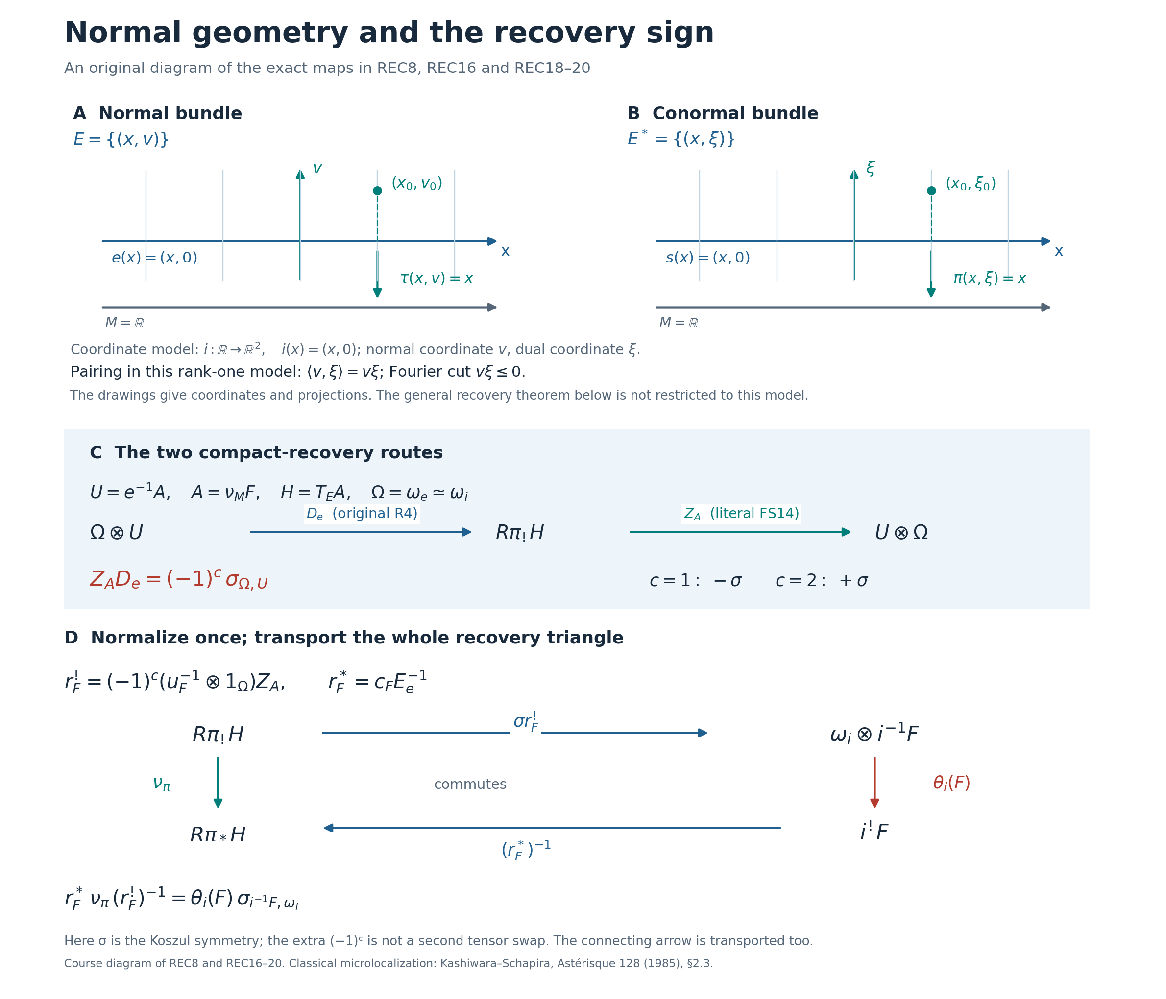
Panels A and B are the coordinate model $i:\mathbb R\hookrightarrow\mathbb R^2$, $i(x)=(x,0)$. The coordinates $v$ and $\xi$ lie in the normal and conormal fibers, with pairing $v\xi$. The blue lines are the zero sections $e$ and $s$; the projections $\tau(x,v)=x$ and $\pi(x,\xi)=x$ land in the separately drawn base $M$. These panels specify coordinates and maps; they assert no metric or numerical bound.

Panels C and D state the general codimension-$c$ comparison proved above, not a restriction to the illustrated rank-one bundle. REC8 gives $Z_AD_e=(-1)^c\sigma_{\Omega,U}$; this parity is additional to the displayed Koszul symmetry. REC16 selects the compact recovery $r_F^!=(-1)^c(u_F^{-1}\otimes1_\Omega)Z_A$. Together with ordinary recovery $r_F^*=c_FE_e^{-1}$, it gives the exact REC18 square. Its lower arrow points left and is $(r_F^*)^{-1}$. REC19 identifies support forgetting with the right-ordered relative trace, and REC20 transports the connecting map with the same normalization.

The diagram uses the assumptions and prerequisite boundary of SH02-MIC-ZERO: arbitrary bounded coefficient complexes over the stated commutative ring of finite global dimension. It adds no field, constructibility, orientability, compactness or noncharacteristic assumption. The locally closed embedding case is obtained by the restriction described above.

This programme diagram depicts REC1–REC20, including the explicit parity comparison proved above. The classical recoveries and boundary triangle are compared with Kashiwara and Schapira, Microlocal Study of Sheaves, Astérisque 128 (1985), §2.3, Proposition 2.3.2 and Corollary 2.3.3, pp. 46–47. That source is credited for the mathematics, not as the source of the diagram or of the course’s parity recipe. A vector copy of the diagram retains the same labels and arrows.

SH02-MIC-CORRESPONDENCE — A map gives two covector arrows

Let $f:Y\to X$, and let $j:N\hookrightarrow Y$ be a closed submanifold with $f(N)\subset M$. Write $g=f|_N:N\to M$. Put $$E_Y=N_NY,\quad E_X=N_MX,\quad C=N\times_M E_X^*.$$ The normal derivative $q:E_Y\to E_X$ factors as $$E_Y\xrightarrow{h}N\times_M E_X\xrightarrow{b}E_X, \qquad h(n,v)=(n,\overline{df}_n v).$$ Its covector correspondence is $$E_Y^*\xleftarrow{r}C\xrightarrow{s}E_X^*, \qquad r(n,\xi)=(n,\overline{df}_n^*\xi), \quad s(n,\xi)=(g(n),\xi). \qquad\text{(MIC8)}$$ Thus $r$ is the transpose of the fibre map $h$, and $s$ changes the base. Both carry the displayed positive transpose; no antipodal map is hidden in MIC8.

For comparison, the ambient correspondence is $$T^*Y\xleftarrow{\rho_f}Y\times_XT^*X\xrightarrow{\varpi_f}T^*X, \qquad \rho_f(y,\xi)=(y,df_y^*\xi).$$ The subset killed by $\rho_f$ is $K_f=\{(y,\xi):df_y^*\xi=0\}$; it is the inverse image of the zero section. Restricting to $N$ and to covectors annihilating $TM$ gives MIC8 because $df(TN)\subset TM$. This direct verification ensures that the maps are correctly typed even if $N\ne f^{-1}M$. Different names for $\rho_f$ and $\varpi_f$ in the literature designate these same two explicit maps.

Let $u:C\to N$ be the base projection and put $$\ell=j^{-1}\omega_f\otimes\omega_g^{\otimes-1}, \qquad L=u^{-1}\ell. \qquad\text{(MIC9)}$$ If the normal ranks are $c_Y,c_X$, then the shift of $\ell$ is $c_Y-c_X$. The tangent exact sequences of $N\subset Y$ and $M\subset X$ identify $$\omega_h=\tau_Y^{-1}\ell,\qquad \omega_r=L^{\otimes-1},\qquad \omega_s=u^{-1}\omega_g. \qquad\text{(MIC10)}$$ Here $\omega_h$ is computed over the identity of $N$. To check MIC10, the orientation of a vector-bundle total space is base orientation times fibre orientation. The base factors cancel for $h$ and $r$. The fibre orientation ratio for $r$ is the dual-bundle ratio in the reverse order; positive dual-orientation identification changes it into the inverse ratio for $h$. The rank differences change sign as well. For $s$, the two normal-fibre factors cancel and leave precisely the orientation of $g$. This proof uses neither injectivity nor constant rank of the normal derivative. The maps of shifted lines are fixed by the unique right-tensor extraction of counit-normalized exceptional transitivity, as in FF3a and MEP3–MEP6. SH02-MEP-NORMAL-COUNITS checks the normal-deformation identification using the time-submersion counits. The coherent inverse pairing and the left-tensor internal-Hom counit are distinguished explicitly; their forward-ordered contractions cannot be substituted for one another in odd relative rank.

SH02-MIC-EXCHANGE — Four Fourier identities for the correspondence

For a conic bounded complex $A$ on $E_Y$ and $H$ on $E_X$, Fourier exchange gives $$\begin{aligned} T_{E_X}Rq_!A&\simeq Rs_!r^{-1}T_{E_Y}A,\\ T_{E_Y}q^!H&\simeq Rr_*s^!T_{E_X}H,\\ T_{E_Y}q^{-1}H&\simeq Rr_!\bigl(L^{-1}\otimes s^{-1}T_{E_X}H\bigr),\\ T_{E_X}Rq_*A&\simeq Rs_*\bigl(r^!T_{E_Y}A\otimes L\bigr). \end{aligned} \qquad\text{(MIC11)}$$ The notation $L^{-1}$ means the tensor inverse complex, including its opposite shift.

Derivation with morphisms fixed. Factor $q=bh$. Fourier commutes with base inverse image and base proper direct image by the Cartesian bundle squares and proper-support base change. For the fibre map $h$, the equality $\langle h(v),\xi\rangle=\langle v,r(\xi)\rangle$ identifies the two closed halfspace kernels. Proper-support composition and projection formula therefore identify $T_{E_X}Rq_!$ with $Rs_!r^{-1}T_{E_Y}$. This is the first isomorphism, with its specified natural map.

Transport this isomorphism across the coherent Fourier equivalences and take its right adjoint mate. The right adjoint of $Rs_!r^{-1}$ is $Rr_*s^!$, yielding the second identity. Applying the same halfspace construction to the transpose and using the Fourier inverse formula with its orientation trace gives $T_{E_Y}(\omega_h\otimes h^{-1}H')\simeq Rr_!T_{N\times_M E_X}H'$. Substitute $H'=b^{-1}H$, commute the invertible base line with the operations, and use MIC10. This yields the third identity, with $L^{-1}$. Its right adjoint is the fourth: the right adjoint of $Rr_!(L^{-1}\otimes s^{-1}(-))$ is $Rs_*(r^!(-)\otimes L)$. These steps are the bundle Fourier comparison proofs in the cited contracts, applied to the displayed maps; they also explain every factor in MIC11.

All four identities use the specified raw Fourier equivalence and its adjunction maps. For precision, the third row is original R4 untwisted by the right-ordered tensor–Hom transpose and then the symmetry putting the line on the left, exactly MEP18. Its right mate is the fourth row: MEP16–MEP20 prove that its contracted endpoint is the inverse of the braided support endpoint FTC13a. Bare uncontracted L3 differs from its right-ordered R4 mate by the relative-rank parity, so an unsigned identification of those two maps is not used. The first and second rows use the primitive proper kernel map and its exceptional mate. The base exchanges then paste as in MEP9–MEP10b. No ordinary direct image is replaced by a proper direct image for a nonproper map.

SH02-MIC-TRACE-EXCHANGE — The two exact comparison identities

For the next two squares with their indicated trace verticals, the following exact compatibilities hold with the completed MIC11 endpoints:

1. Under MIC11, the transform of $Rq_!A\to Rq_*A$ agrees with $$Rs_!r^{-1}T_{E_Y}A \longrightarrow Rs_!(r^!T_{E_Y}A\otimes L) \longrightarrow Rs_*(r^!T_{E_Y}A\otimes L),$$ where the first arrow uses the relative-trace comparison for $r$, tensored by $L=\omega_r^{-1}$, and the second forgets proper support.

2. Under MIC11 and $\omega_q=\tau_Y^{-1}j^{-1}\omega_f$, the transform of $\omega_q\otimes q^{-1}H\to q^!H$ agrees with $$Rr_!(u^{-1}\omega_g\otimes s^{-1}T_{E_X}H) \longrightarrow Rr_!s^!T_{E_X}H \longrightarrow Rr_*s^!T_{E_X}H,$$ where the first arrow is the relative-trace comparison for $s$ and the second forgets proper support.

These are equalities of particular natural transformations. MEP11 proves the first by the complete FGC support equation and support-compatible base exchange; MEP20 identifies its endpoint with the actual ordinary adjoint mate. MEP14 proves the second by the original R2/R4 trace equation FTE34, the base trace counit square, and the exact composite trace formula. MEP5 and SH02-MEP-NORMAL-COUNITS identify the actual normal orientation maps, while MEP10a–MEP10b give both full input and output comparisons. These proofs retain the original arrows and every orientation factor. They are relative to the finite operation and specialization inputs stated in SH02-MEP-SCOPE.

SH02-MIC-DIRECT — Pushing forward a normal limit

For $G\in D^b(k_Y)$, there is a commuting square $$\begin{array}{ccc} Rs_!r^{-1}\mu_NG&\xrightarrow{a_G}&\mu_M(Rf_!G)\\ \downarrow&&\downarrow\\ Rs_*(r^!\mu_NG\otimes L)&\xleftarrow{d_G}&\mu_M(Rf_*G). \end{array} \qquad\text{(MIC12)}$$ The right vertical map forgets proper support. For the left vertical map, the trace comparison $r^{-1}A\otimes\omega_r\to r^!A$, tensored by $L=\omega_r^{-1}$, gives $r^{-1}A\to r^!A\otimes L$. Apply $Rs_!$, then forget proper support. This description specifies the arrow even when it is not invertible.

Proof. Apply $T_{E_X}$ to the specialization square $$\begin{array}{ccc} Rq_!\nu_NG&\longrightarrow&\nu_MRf_!G\\ \downarrow&&\downarrow\\ Rq_*\nu_NG&\longleftarrow&\nu_MRf_*G. \end{array}$$ Substitute the first and fourth identities of MIC11. This produces a commuting square with the transported left vertical arrow. Part 1 of SH02-MIC-TRACE-EXCHANGE is proved by MEP11 with the actual mate endpoint MEP20. It identifies the transported arrow with the displayed relative-trace and support-forgetting composite. $\square$

All four arrows of MIC12 are isomorphisms under the following three support conditions, where support means closed support:

1. $f:\operatorname{supp}(G)\to X$ is proper.
2. $q:C_N(\operatorname{supp}G)\to E_X$ is proper.
3. $\operatorname{supp}(G)\cap f^{-1}(M)\subset N$.

Indeed these are exactly the three conditions under which all arrows of the specialization square are isomorphisms; applying an equivalence and the isomorphisms MIC11 preserves this property. None of the conditions is discarded merely because $f$ is proper. In particular, if $N=f^{-1}M$, $f$ is clean with respect to $M$, and $f$ is proper on $\operatorname{supp}(G)$, the normal-geometry properness lemma supplies condition 2 and the other two are immediate. Clean means that $N$ is a submanifold and its normal derivative into the pulled-back normal bundle is injective.

SH02-MIC-INVERSE — Pullback has two comparison directions

For $F\in D^b(k_X)$, there is a commuting square $$\begin{array}{ccc} Rr_!(u^{-1}\omega_g\otimes s^{-1}\mu_MF) &\xrightarrow{c_F}&\mu_N(\omega_f\otimes f^{-1}F)\\ \downarrow&&\downarrow\\ Rr_*s^!\mu_MF&\xleftarrow{b_F}&\mu_N(f^!F). \end{array} \qquad\text{(MIC13)}$$ The right vertical map is $\mu_N$ applied to the trace comparison $\omega_f\otimes f^{-1}F\to f^!F$. The left vertical map first uses $s^{-1}H\otimes\omega_s\to s^!H$, where $\omega_s=u^{-1}\omega_g$, and then the morphism $Rr_!\to Rr_*$.

Proof. The normal deformation orientation comparison gives $\omega_q=\tau_Y^{-1}j^{-1}\omega_f$. Specialization has a commuting square from its ordinary inverse comparison $q^{-1}\nu_MF\to\nu_Nf^{-1}F$, its exceptional inverse comparison $\nu_Nf^!F\to q^!\nu_MF$, and the two trace comparisons. Apply $T_{E_Y}$. The second identity of MIC11 gives the lower row of MIC13. For the upper left object, the third identity gives $$T_{E_Y}(\omega_q\otimes q^{-1}\nu_MF) \simeq Rr_!(u^{-1}j^{-1}\omega_f\otimes L^{-1} \otimes s^{-1}\mu_MF) \simeq Rr_!(u^{-1}\omega_g\otimes s^{-1}\mu_MF).$$ The last cancellation is MIC9. A locally constant orientation complex commutes with specialization, by local trivialization and the projection formula, so the upper right object is the one displayed. The transformed specialization square commutes with its transported vertical arrow. Part 2 of SH02-MIC-TRACE-EXCHANGE is MEP14: the exact composite uses the trace for $s$ inside $Rr_!$, then forgets proper support. Its input and output comparisons are the original R4 and R2 maps in MEP10b. Thus the claimed square commutes with this explicit trace vertical. $\square$

SH02-MIC-SMOOTH — When both maps of manifolds are smooth

If $f:Y\to X$ and $g:N\to M$ are smooth, all four maps of MIC13 are isomorphisms. To see the geometry, surjectivity of $df$ makes the normal fibre map $h$ surjective, and $g$ is a submersion on the base. Thus $q$ is smooth. The specialization inverse comparisons are isomorphisms on the smooth locus of $q$, which here is its entire domain. Moreover $r$ is a closed vector-bundle embedding, so $Rr_!=Rr_*$; the trace comparison for the smooth base map $s$ and that for $f$ are isomorphisms. Either this argument or the whole transformed specialization square proves the assertion.

The ambient transpose $\rho_f$ identifies $Y\times_XT^*X$ with a vector subbundle of $T^*Y$. Its intersection over $N$ with $E_Y^*$ corresponds exactly to $C=N\times_ME_X^*$. Indeed $df_y^*\xi$ annihilates $T_yN$ if and only if $\xi$ annihilates $df_y(T_yN)$. Smoothness of $g$ makes this image $T_{f(y)}M$. Hence the condition is precisely $\xi\in E_X^*$. This also identifies the conormal map $s$ in the ambient correspondence.

SH02-MIC-TRANSVERSE — The transverse ordinary inverse map

Suppose $f$ is transverse to $M$ and $N=f^{-1}M$. Then the normal fibre map $h$ is an isomorphism. Consequently $r$ is an isomorphism and MIC9 identifies $j^{-1}\omega_f\simeq\omega_g$. Cancel this invertible coefficient complex in the upper row of MIC13. The result is a natural morphism $$Rr_*s^{-1}\mu_MF\longrightarrow\mu_N(f^{-1}F). \qquad\text{(MIC14)}$$ Here $Rr_!=Rr_*$ because $r$ is an isomorphism. Transversality alone has not made this morphism an isomorphism: $f$ need not be smooth. Additional microlocal criteria for invertibility belong to later microsupport estimates.

SH02-MIC-ADJUNCTIONS — Checking the actual comparison maps

The next two identities express the compatibility of MIC12 and MIC13 with adjunction. They are useful because agreement of the four objects in a square does not establish agreement of its arrows.

Set $$\mathcal A=Rs_!r^{-1},\qquad \mathcal B=Rr_*s^!, \qquad \mathcal D=Rr_!(L^{-1}\otimes s^{-1}(-)),\qquad \mathcal C=Rs_*(r^!(-)\otimes L).$$ These are adjoint pairs $\mathcal A\dashv\mathcal B$ and $\mathcal D\dashv\mathcal C$. Canceling the orientation in the upper row of MIC13 gives a map $\widetilde c_F:\mathcal D\mu_MF\to\mu_Nf^{-1}F$. The lower inverse map $b$ is the mate of the upper direct map $a$. The lower direct map $d$ is the mate of $\widetilde c$.

For clarity, the first of these assertions means the explicit equality $$b_F: \mu_Nf^!F\xrightarrow{\eta_{\mathcal A}} \mathcal B\mathcal A\mu_Nf^!F \xrightarrow{\mathcal B a_{f^!F}} \mathcal B\mu_M Rf_!f^!F \xrightarrow{\mathcal B\mu_M\varepsilon_f} \mathcal B\mu_MF. \qquad\text{(MIC15)}$$ The second means $$d_G: \mu_MRf_*G\xrightarrow{\eta_{\mathcal D}} \mathcal C\mathcal D\mu_MRf_*G \xrightarrow{\mathcal C\widetilde c_{Rf_*G}} \mathcal C\mu_Nf^{-1}Rf_*G \xrightarrow{\mathcal C\mu_N\varepsilon_f'} \mathcal C\mu_NG. \qquad\text{(MIC16)}$$ Here $\eta$ denotes the indicated unit; $\varepsilon_f$ and $\varepsilon_f'$ are the counits of $Rf_!\dashv f^!$ and $f^{-1}\dashv Rf_*$, respectively.

Why these are the maps already constructed. On the normal deformation spaces, specialization’s exceptional inverse comparison is obtained by inserting the $Rq_!\dashv q^!$ unit, then its direct comparison, then the $Rf_!\dashv f^!$ counit. Its ordinary direct comparison is obtained by inserting the $q^{-1}\dashv Rq_*$ unit, then its inverse comparison, then the $f^{-1}\dashv Rf_*$ counit. These descriptions can equally be checked by moving their deformation base-change squares across the corresponding adjunctions: proper base change and its exceptional mate insert exactly those units and counits. Fourier exchange in MIC11 uses those same mates. MEP16–MEP20 check the full orientation extraction in the ordinary pair, so this statement does not assume the false unsigned identification of bare L3 with the right-ordered R4 mate. Transporting the two composites therefore gives MIC15 and MIC16, including their order and orientation evaluations. This is the place where coherent mate constructions, rather than arbitrary isomorphisms from inversion, are required.

Now let $\varphi:G\to f^!F$ and let $\overline\varphi:Rf_!G\to F$ be its adjoint. Then the square $$\begin{array}{ccc} \mathcal A\mu_NG&\xrightarrow{a_G}&\mu_MRf_!G\\ \mathcal A\mu_N(\varphi)\downarrow&&\downarrow\mu_M(\overline\varphi)\\ \mathcal A\mu_Nf^!F&\xrightarrow{\varepsilon_{\mathcal A}\circ\mathcal A b_F}&\mu_MF \end{array} \qquad\text{(MIC17)}$$ commutes. To prove it, substitute MIC15 into the lower horizontal map. Naturality permits moving the counit past $\mathcal A\mathcal B a$; the triangular identity $\varepsilon_{\mathcal A}\circ\mathcal A\eta_{\mathcal A}=1_{\mathcal A}$ then cancels the inserted unit. The lower map becomes $\mu_M\varepsilon_f\circ a_{f^!F}$. Naturality of $a$ with respect to $\varphi$ makes its composite with the left side equal to $\mu_M(\varepsilon_f\circ Rf_!\varphi)\circ a_G$, which is the right-hand route because the expression in parentheses is $\overline\varphi$.

Similarly, for $\psi:F\to Rf_*G$ with adjoint $\overline\psi:f^{-1}F\to G$, let $c'_F=\mathcal C\widetilde c_F\circ\eta_{\mathcal D}:\mu_MF\to\mathcal C\mu_Nf^{-1}F$. Then $$\begin{array}{ccc} \mu_MF&\xrightarrow{c'_F}&\mathcal C\mu_Nf^{-1}F\\ \mu_M(\psi)\downarrow&&\downarrow\mathcal C\mu_N(\overline\psi)\\ \mu_MRf_*G&\xrightarrow{d_G}&\mathcal C\mu_NG \end{array} \qquad\text{(MIC18)}$$ commutes. Substitute MIC16. Naturality of the unit and of $\widetilde c$ moves $\psi$ through the first two arrows. The remaining composite is $\varepsilon_f'\circ f^{-1}\psi=\overline\psi$, giving the other route. This proves both adjunction identities for arbitrary bounded inputs, without a constructibility or properness assumption.

SH02-MIC-EXTERNAL — Independent variables and external tensor products

Let $M\subset X$, $N\subset Y$ be closed submanifolds and let $F\in D^b(k_X)$, $G\in D^b(k_Y)$. There is a natural morphism $$\mu_MF\boxtimes^L\mu_NG \longrightarrow\mu_{M\times N}(F\boxtimes^LG) \qquad\text{(MIC19)}$$ on $N_M^*X\times N_N^*Y$.

Proof. The normal bundle of the product embedding is $N_MX\times N_NY$. The specialization product comparison is $\nu_MF\boxtimes^L\nu_NG\to\nu_{M\times N}(F\boxtimes^LG)$. Each factor is conic in its own normal variable, so their external product is invariant under the two independent positive scalings. The Fourier product theorem identifies the transform of its left side with $\mu_MF\boxtimes^L\mu_NG$. Apply Fourier to the comparison and compose with that isomorphism. This constructs MIC19 and proves its naturality. The use of independent conicity is necessary for the Fourier product theorem; it follows here from the two separate specializations. The specialization comparison is not asserted to be invertible in general, so neither is MIC19. $\square$

SH02-MIC-CONVOLUTION — Addition of covectors tests a tensor product

For one embedding $M\subset X$, let $\gamma:E^*\times_M E^*\to E^*$, $\gamma(\xi,\eta)=\xi+\eta$. For complexes on bundles over the same base, $A\boxtimes_M^LB$ means the tensor product of their two inverse images to the fibre product. There is a natural morphism $$R\gamma_!(\mu_MF\boxtimes_M^L\mu_MG) \longrightarrow\mu_M(F\otimes^LG)\otimes\pi^{-1}\omega_i. \qquad\text{(MIC20)}$$ In particular the proper direct image, the positive sum, and the codimension shift in $\omega_i$ are part of the formula.

Proof. Let $\delta:E\hookrightarrow E\times_M E$ be the diagonal. Its transpose is the positive sum $\gamma$, since $\langle(v,v),(\xi,\eta)\rangle=\langle v,\xi+\eta\rangle$. The normal bundle of $\delta$ is identified with $E$ by the difference of the second coordinate and the first. Consequently $\omega_\delta=\tau^{-1}\operatorname{or}_{M/X}[-c]=\tau^{-1}\omega_i$, with this ordered orientation convention.

Apply the oriented Fourier inverse-image identity to $\delta$, then the product identity to $A=\nu_MF$, $B=\nu_MG$. It gives $$\begin{aligned} R\gamma_!(\mu_MF\boxtimes_M^L\mu_MG) &\simeq T_E\bigl(\omega_\delta\otimes \delta^{-1}(A\boxtimes_M^LB)\bigr)\\ &\simeq T_E(A\otimes^LB)\otimes\pi^{-1}\omega_i. \end{aligned}$$ The specialization tensor map $A\otimes^LB\to\nu_M(F\otimes^LG)$, obtained by its external comparison and the ordinary inverse comparison along the diagonal, now gives MIC20 after applying $T_E$. All tensor products remain in the bounded range because the coefficient ring has finite global dimension. Neither tensor comparison has been replaced by an isomorphism. $\square$

SH02-MIC-EXAMPLES — Three checks with arbitrary coefficient modules

Let $A$ be any bounded complex of $k$-modules. The examples apply to torsion and infinitely generated coefficients as well as to free ones.

A locally constant ambient complex. If $F$ is locally constant on a neighborhood of $M$, then $$\mu_MF\simeq s_*(i^{-1}F\otimes\omega_i).$$ In normal coordinates its specialization is $\tau^{-1}i^{-1}F$. For a nonzero covector, the negative Fourier slice is a closed halfspace of a positive-dimensional vector space; its compactly supported cohomology vanishes. At the zero covector it is the entire normal fibre, whose orientation trace is $\operatorname{or}_{M/X}[-c]$. Restriction to the closed zero section constructs the isomorphism, and the local orientation traces glue. Thus the third term of MIC7 is zero, as it must be when the two zero-direction recoveries agree by the local orientation calculation.

A complex supported on the submanifold. If $F=i_*A_M$, where $A_M\in D^b(k_M)$ is arbitrary, then $$\nu_M(i_*A_M)=e_*A_M,\qquad \mu_M(i_*A_M)=\pi^{-1}A_M.$$ In a deformation chart the positive lift of the support is exactly the zero normal vector at each positive parameter. Its closure meets the central fibre in the zero section, and the interval limit of its base-pulled coefficient is $A_M$. This proves the first formula, including its extension by zero. In the Fourier kernel the pairing at the zero normal vector is always zero; the projection of this supported correspondence to $E^*$ is the identity over $M$. Proper base change therefore gives the second formula with no shift. The two checks are $R\pi_*\pi^{-1}A_M=A_M$ and $R\pi_!\pi^{-1}A_M=A_M\otimes\operatorname{or}_{M/X}[-c]$, precisely MIC6.

Changing whether a boundary is included. Take $X=\mathbb R$, $M=\{0\}$, with its usual orientation. For constant-extension sheaves on rays, $$\mu_0(k_{[0,\infty)}\otimes^LA)=k_{(0,\infty)}\otimes^LA, \qquad \mu_0(k_{(0,\infty)}\otimes^LA)=k_{(-\infty,0]}\otimes^LA[-1].$$ Both inputs are already conic and identify with their normal specializations: the deformation of a vector space along zero has coordinates $(v,t)$ with $p(v,t)=tv$; on $t>0$, scalar transport identifies $p^{-1}F$ with the pullback of $F$ from $v$. The boundary limit is then $F$, by interval cohomology. In the first case a positive covector leaves only the point zero in the negative-pairing slice, while a nonpositive covector leaves the closed ray, with vanishing compactly supported cohomology. In the second case a positive covector leaves an empty slice and a nonpositive covector leaves the open ray, whose compactly supported trace is $k[-1]$. The canonical cone-transform maps give the stated open or closed extensions, including their stalk maps at zero. This is why changing an endpoint changes both the side and the shift.

SH02-MIC-PROBLEMS — Exercises with complete solutions

Problem 1. In codimension zero, identify $\mu_M$, where $M$ is an open and closed component of $X$, and evaluate MIC7.

Solution. The normal bundle has rank zero and is $M$ itself. Specialization is ordinary restriction to that component, and the rank-zero Fourier kernel is the identity. Thus $\mu_MF=i^{-1}F=i^!F$. The orientation complex $\omega_i$ is $k_M$, the punctured bundle is empty, and MIC7 is $i^{-1}F\xrightarrow{1}i^{-1}F\to0\to$. The unit and counit of restriction to an open and closed component identify its first arrow with the identity.

Problem 2. Test the orientation in MIC20 with $X=\mathbb R^d$, $M=\{0\}$, and $F=G=k_{\{0\}}$. What goes wrong if $R\gamma_!$ is replaced by $R\gamma_*$?

Solution. Both microlocalizations are $k_{(\mathbb R^d)^*}$. The fibre of addition is an affine $d$-space, with compactly supported cohomology $k[-d]$ after choosing the usual orientation. Hence the left side is $k_{(\mathbb R^d)^*}[-d]$. The right side has the same shift because $F\otimes G=k_{\{0\}}$ and $\omega_i=k[-d]$. The map is the fibre orientation trace in this model and is an isomorphism. Ordinary direct image instead gives $k$ in degree zero along each fibre. For $d>0$ it therefore fails this equality by exactly $d$ degrees.

Problem 3. Suppose $p=0_x$. Explain why MIC4 cannot use the condition $\langle v,p\rangle\geq0$ in place of strict positivity away from zero.

Solution. A weak inequality at $p=0$ admits every closed support, including $Z=X$. With support enlargement, this last support is terminal, so the resulting colimit is $H^r(F)_x$. The actual zero-direction object is $i^!F$. For $X=\mathbb R$, $M=\{0\}$, and $F=k_X$, it is $k[-1]$, whereas the weakened test gives $k$. Strict positivity excludes every nonzero normal vector and restores the exceptional, rather than ordinary, restriction.

Problem 4. Let $f:Y\to X$ and $g:N\to M$ be smooth. Prove directly that the transpose normal map $r$ in MIC8 is a closed embedding, and identify the two reasons the left vertical arrow in MIC13 is invertible.

Solution. For any class in $T_{f(n)}X/T_{f(n)}M$, choose a representative in $T_{f(n)}X$ and lift it through the surjective map $df_n$. Its class in $T_nY/T_nN$ maps to the desired normal class. Thus $h$ is fibrewise surjective. A smooth surjective map of vector bundles has a locally split kernel and its transpose is an injective map onto a subbundle, which is closed in each local trivialization and hence globally closed. This proves $r$ is a closed embedding, so $Rr_!=Rr_*$. Also $s$ is the base change of the smooth map $g$, so $s^{-1}H\otimes\omega_s\to s^!H$ is an isomorphism. These are exactly the two constituents of the left vertical map.

Problem 5. Give the map $\mu_MF\to\mathcal C\mu_Nf^{-1}F$ without saying merely that it is obtained by adjunction, and verify its compatibility with a map $F\to Rf_*G$.

Solution. The map is $\mu_MF\xrightarrow{\eta_{\mathcal D}}\mathcal C\mathcal D\mu_MF \xrightarrow{\mathcal C\widetilde c_F}\mathcal C\mu_Nf^{-1}F$. For $\psi:F\to Rf_*G$, naturality of $\eta_{\mathcal D}$ moves $\psi$ past the first arrow and naturality of $\widetilde c$ moves it past the second. Following by $\mathcal C\mu_N\varepsilon_f'$ then produces $\mathcal C\mu_N(\varepsilon_f'\circ f^{-1}\psi)$, the adjoint of $\psi$. This is exactly MIC18. There is no scalar or unspecified isomorphism left to choose.