Causal kernels, initial data, and short-time geometry
A wave kernel has two useful descriptions. In frequency space it solves an ordinary differential equation with prescribed initial data. In physical space its singularities sit on a cone. The frequency description fixes constants and initial traces; the cone description explains which parts of a local geometric construction can influence a short time interval. We develop both descriptions before introducing variable coefficients.
The spatial dimension is any integer . The variable-coefficient construction also permits complex matrix lower-order coefficients, without diagonalizing them. Its principal symbol must be a positive scalar quadratic form times the identity. A general system with several characteristic speeds is a different problem.
1. Conventions and the causal distribution problem
For spatial Fourier transformation use The same convention applies in time. Set Distributions supported in will be called causal. Reflection means ; for the radial kernels below it equals .
The Fourier inversion and distribution extension inputs are proved in Sections1–2 of Fourier transforms, finite spectra and convex separation. The elementary integrations, gamma and beta identities, dominated holomorphic derivatives and identity theorem have their complete proof locators CX1–CX11 and CX29–CX40 in Sections16.1–16.10 of Singularities along a submanifold and smooth boundary passage. The finite-pole rectangle case of the residue theorem used here, including its contour orientation and deformation, is proved in Section4.1 from those circle and triangle proofs. The added contour pieces are estimated there after testing, and Section5 supplies the Gaussian spatial regularization. The beta and gamma normalizations used here are displayed in the proof. The distributional inputs are distributional derivatives, multiplication by smooth functions, changes of variables by diffeomorphisms, compact-support distribution estimates, and the wavefront pullback theorem for a submersion with its converse in product coordinates. For wavefront sets we additionally use the exact constant-coefficient microlocal ellipticity implication where is the principal symbol, and the parameter theorem that absence of covectors normal to the parameter fibers gives smooth distribution-valued dependence. The coordinate, submersion and parameter-smoothness statements are proved in Sections18.3–18.6, WF5–WF17, of Detecting regularity without choosing coordinates. Its Sections18.7–18.8, WF18–WF34, prove the full differential elliptic regularity statement and its independent odd-wave receiving comparison. No propagation theorem or global wave existence theorem is needed.
The jointly smooth exponential chart, radial distance identity and full transformed drift are proved in Sections17.8–17.10, NG0–NG7, of Detecting regularity without choosing coordinates. Section9 below proves their precise wave receiving comparison and the complete ordered matrix transport independently. All estimates for the causal distributions themselves are proved below. The later elliptic and reflected constructions are comparison targets, rather than prerequisites for this proof.
When a time distribution is viewed as a function of a spatial parameter, continuity into distributions of order at most means the following local statement: it acts on compactly supported tests, the pairings are continuous in the parameter, and on compact parameter sets they obey a common -seminorm bound. This weak finite-order continuity does not assert operator-norm continuity on the dual of .
2. A Laplace calculation that constructs the whole family
There is an entire distribution family , supported in , whose Fourier–Laplace transform is The integral denotes distributional pairing, equivalently the Fourier transform of the exponentially damped distribution. The power is determined by continuation from positive and . The family satisfies
Proof. We first justify the gamma normalization for complex parameters. For , let , using the real logarithm for positive . For an integer , repeated integration by parts in the beta integral gives For the rational identity, one integration replaces the integral by times the integral with parameters ; the final integral is . No gamma division is used. For the limit put . On a compact subset of the right half-plane choose . The resulting integrands are bounded in absolute value by , since for . Pointwise convergence is uniform for in that compact set, and the integrable bound makes the integral convergence locally uniform.
Define . The numbers decrease and are bounded below: the decrease follows from , and comparison with the integral of gives the lower bound. Write their limit as . The exact reciprocal of the scaled beta expression in (W4a) is the entire finite product Its limit exists locally uniformly on the whole plane. Indeed, on choose an integer . For , use the logarithm defined by its power series at one; then Thus the sum of these tail logarithms converges uniformly on this disk. The derivative of each tail logarithm is , uniformly ; uniform convergence of this derivative series also proves that the tail sum is holomorphic. Exponentiating it, and retaining the first factors as polynomials times exponentials, proves local uniform convergence to an entire function The exponential of the tail sum never vanishes. Consequently the finite initial factors show that the only zeros are , each simple: near any of these points precisely one polynomial factor has a simple zero and all the others are nonzero. This argument uses logarithms only for the tail factors close to one, including when the disk contains zeros of the full product.
For , the product of and is exactly one. Passing to the two locally uniform limits gives ; in particular the gamma integral has no zero there. This identifies as the entire reciprocal of the meromorphic continuation of gamma, with the constant fixed by the original integral, rather than only up to a nonzero factor. Explicitly , so . Integration by parts in the gamma integral gives in the right half-plane. It follows that there, hence everywhere by the identity theorem. Iterating at , for an integer , gives For this derivative, differentiate at and use ; its reciprocal has the stated residue. These facts justify both complex gamma normalizations below and the pole cancellation in Section 3.
Initially suppose . The locally integrable function has locally integrable cone boundary because the exponent is greater than . At the vertex, radial integration in gives a power , which is integrable by the other inequality. On compact subsets of this half-plane the same estimates hold after inserting any fixed power of . Thus (W6) is holomorphic as a distribution there.
At , put . The elementary ball integral, obtained by polar coordinates and , is For the two half-intervals give the same formula. The time integral is . Their product with the constant in (W6) is , because The full beta and Gaussian calculation CX36–CX38 in the earlier conormal lesson proves (W7) and (W8), retaining their original substitutions, sphere densities and all factors of two and pi. Section2.1 records the exact receiving domains and continuation.
To retain the spatial frequency, first replace by a real vector with . The integral with weight is absolutely convergent. Rotate onto the first spatial axis, and in the -plane make a real linear change preserving , the future cone, and determinant one. Explicitly its coefficients are and . It transforms the linear form into . The preceding evaluation is therefore . Both sides are holomorphic for complex with . Successive one-variable identity theorems extend their equality from a real neighborhood to that tube. Taking proves (W4) in the initial range.
For larger real part, ordinary distributional differentiation, including the boundary where the function and the necessary traces vanish, gives Indeed , , , and the difference of the squared gradients is . The gamma functional equation makes the constants in (W6) satisfy . The identity then holds throughout the initial half-plane by holomorphic continuation. For arbitrary , choose an integer so that is in that half-plane and define The recursion shows that different choices give the same result. This constructs an entire family, since it constructs it holomorphically on successively larger half-planes. Its support remains in . Its members are tempered: (W6) has polynomial growth, and (W10) applies only finitely many derivatives. On the cone, exponential damping makes their transforms meaningful; differentiation proves (W4) for (W10). Fourier injectivity then proves . Homogeneity follows by scaling (W6), then applying (W10); the degree decreases by two at each application of . This also checks the vertex in (W5), not merely points with positive time.
For every integer , define If , (W4), with the time frequency on the line , gives the contour formula The right side is a distributional inverse Fourier–Laplace transform. It is not an absolutely convergent integral at arbitrary dimension. For fixed , the denominator is nowhere zero on the real integration variables and its inverse and derivatives have polynomial growth, so the inverse transform exists. Formula (W4) identifies it with (W11) for every , proving independence of the contour height. In particular the support is the full causal cone condition , including its vertex, rather than merely .
2.1. The full damping, branch and continuation maps
The integration and complex analysis used above have complete earlier proofs: Singularities along a submanifold and smooth boundary passage, CX1–CX11 proves the circle formula, identity theorem and every dominated complex derivative; CX29–CX40 proves the gamma product, beta substitution, duplication, sphere density and Laplace branch. In particular CX36 retains the substitution and its Jacobian . CX37 evaluates by and then , giving exactly (W8); CX38 gives exactly (W7), including dimension one. These are proof inputs with specified receiving formulas, rather than citations offered in place of those calculations.
Here are the additional analytic details needed for the distribution construction. On a compact set of complex parameters choose one integer so that every is in the original convergence region. Write . On its compact parameter set and , with positive margins. In the integral (W6) use . Its absolute spatial integral, with a bounded test inserted, is bounded by a constant times . The constants are uniform on that compact parameter set: the positive power margin bounds the integral at the sphere boundary, and the reciprocal gamma factors are bounded there. For use the smallest exponent, and for the largest. Choosing a Schwartz decay exponent larger than the latter exponent plus one proves a fixed Schwartz seminorm estimate. For (W10), apply that estimate to the full derivative , retaining its finite expansion and all coefficients. This proves temperedness and locally uniform finite-order bounds for the entire family. Logarithmic parameter derivatives have the same estimates after reducing those positive margins; for every fixed integer , is bounded on . The dominated holomorphic integral proof just cited therefore applies to every compact parameter set and every Schwartz test.
In (W9) one may initially take . The cone expression, extended by zero, is then away from the vertex, with its first two boundary jets zero. At the vertex its derivatives of order at most two are bounded by constants times , times bounded annular derivatives, and the corresponding lower-order bounds prove their actual derivatives there by difference quotients. Thus it is there as well. Ordinary differentiation consequently gives the distributional recursion with no boundary or vertex term in this region. Holomorphic continuation of each tested identity supplies the recursion in the original half-plane and makes the definitions (W10) agree on every overlap. Derivatives preserve support; applying this to every test outside proves the complete causal support claim for every parameter.
Exponential damping is an actual Schwartz multiplier after a harmless extension off the support. Choose a smooth scalar cutoff equal to one for and zero for . For , and all its derivatives are bounded, and multiplication preserves every Schwartz seminorm by the full product rule. Its value and all derivatives coincide with on a neighborhood of , so the damped distribution is independent of this cutoff. This defines the damping of every derivative in (W10), without treating an exponentially growing function on negative time as a Schwartz multiplier.
The boost calculation also fixes the complex branch. Write , where are real and . Then
Thus the power in that tube is the holomorphic right-half-plane branch, agreeing with the positive real value at . On a compact sub-tube the integrand is bounded by its original cone power times ; all fixed -derivatives add only powers of , bounded by powers of on the cone. This is an integrable common envelope at infinity and at zero. Successive one-variable identity theorems on a small product of disks extend the equality from a real ball to a complex neighborhood. Equality then extends over the connected tube: along a polygonal path inside it, use a finite chain of overlapping product disks and their convergent local power series. This proves the stated equality on the whole tube and the substitution .
Now retain a complex damping parameter with . For real , the number never lies on the nonpositive real axis: its imaginary part is , and if this vanishes then is positive real. The integral is holomorphic in , with the same exponential envelopes on compact subsets. Continuation from real gives
For initial parameters this follows by absolutely integrable testing. Multiplication by the polynomial is precisely the Fourier transform of the damped operator , since on distributions supported in ; the cutoff derivatives vanish near their support. This proves (WA2) for the continuation (W10). At its full spacetime Fourier transform is one. The Fourier inverse proved in the prerequisite lesson gives ; multiplication on compact tests by gives . This uses the full time frequency as well as the spatial frequency, and fixes the point source exactly.
In (W12) put , retaining the original time variable in its exponential. For , If , the first square is at least , whose sum with the second term is ; otherwise the second term alone is at least . Thus the denominator has a uniform positive bound. Every derivative of its reciprocal is its original polynomial numerator divided by a positive power of that denominator, so it has polynomial growth. The inverse Fourier transform is therefore a tempered distribution before undoing damping, and (WA2) identifies the resulting distribution on compact tests with (W11). This proves the contour formula and its height independence without an untested integral rearrangement.
The Taylor subtraction used for (W13) can likewise be written with all endpoint terms. For an integer , put . The exact pairing is The first integral converges for , the second is entire, and the displayed simple poles are exactly canceled by the proved simple zeros of . On overlapping half-planes the expression agrees with the original integral, hence agrees everywhere by its tested identity theorem. Taylor’s integral remainder bounds it by a finite test seminorm on each compact parameter set. This proves the entire distribution family, its support and its finite-order estimates. Integration by parts on the initial half-plane gives the derivative identity; analytic continuation and differentiation of the Heaviside distribution give every delta derivative in (W13). No divergent endpoint integral is assigned a value.
3. Cone formulas and exact recursion
Let for . Its entire continuation is determined by The entire reciprocal gamma function and its simple zeros were proved in Section 2. For completeness, integrate the initial definition against a compactly supported smooth test after subtracting its Taylor polynomial at zero. The remainder is , so its integral continues to ; the removed monomials give simple fractions in , whose poles are canceled by . Increasing gives the entire family. Integration by parts proves the first identity initially, hence everywhere. This construction also gives for .
Write On the open set , At nonzero points of , the map is a submersion, so this is a legitimate distributional pullback. At the vertex (W15) is interpreted by the construction of Section 2, not by substituting into a singular one-dimensional distribution at a critical point. To prove (W15), use (W6) in its initial range, restrict to , and apply the compatible differential continuations (W10) and (W13). The chain-rule calculation in (W9), now in normalized form, reads There is no claim that (W16) discards the vertex term in the fundamental solution. That term was fixed separately by (W5).
The global recursions, including every vertex contribution, are The first two follow from (W5). For the last, apply spatial Fourier–Laplace transformation. Multiplication by becomes , and The identity follows by injectivity; it therefore has no possible omitted distribution supported at the origin. The degree of homogeneity of is .
4. Initial traces from a Volterra problem
Each , restricted to nonnegative time, is a one-sided function of with values in . Its initial traces are These are traces of the one-sided function. Repeatedly differentiating its extension by zero to negative time can also produce distributions at .
Proof. Put , and define For , its Volterra convolution with a function is . Differentiating twice proves , with zero initial value and derivative. Its Laplace transform is . Hence (W4) implies All interchanges here can first be made after multiplying the spatial transform by a Schwartz cutoff; the bounds below then permit its removal.
There is a useful version on a fixed simplex. For , integrate over , , and put . With the evident single factor interpretation for , This follows by changing the time variables in the convolution to . The removable quotients have value one at zero. Their derivatives in real obey polynomial bounds in on bounded time intervals; for example . Thus each has a bound times a fixed polynomial in . Every compactly supported smooth spatial test has a rapidly decreasing Fourier transform, so inversion and dominated differentiation yield all one-sided distributional derivatives. Uniformity over bounded sets of tests follows from their common Fourier decay seminorms, giving the strong distribution topology as well.
At zero, the simplex integral is One proves this by successively applying , beginning with parameters all equal to two. Therefore the first nonzero Taylor term in (W22) is . Its inverse spatial Fourier transform is exactly (W19). The same expression extends to an odd smooth distribution-valued function on all real , namely The distinction between this odd extension and the causal extension will be essential when time distributions are restricted at a spatial point.
4.1. The simplex factor and the orientation of the tested contour
For completeness the simplex constant in (W23) follows by a finite induction with every factor present. Let denote its integral and . Fix ; in the remaining simplex write , . The remaining factors contribute , their independent integration variables contribute , and the first factor contributes . Hence The beta identity CX36 applies with its positive real parameters . This gives all initial jets in (W19) and the odd extension (W24), including , whose simplex is a point of mass one.
Here is the complete contour estimate used in Section 5. If is supported in with , put . Integration by parts times, with zero endpoint jets, gives on the fixed lower strip , the same bound holds with instead of . Take a rectangle with bottom on , vertical sides at , top at , and . On its added sides the functions and are bounded by constants times and , respectively. Their side lengths are at most ; (WA7) makes all added integrals tend to zero. The bottom runs from left to right, so this closure is positively oriented. To make the finite-pole step explicit, expand the entire tested exponential at each of the two poles, subtract its complete principal parts, and use CX7 to see that the remainder extends holomorphically there. Its rectangle integral is zero by a two-triangle subdivision and CX3. A principal part of order greater than one has its actual single-valued power primitive and contributes zero. For the simple part inside the rectangle, remove a small polygonal disk around the pole and triangulate the region between the two polygons; all interior edges cancel. Let the inner polygons tend to the positively oriented circle: continuity of the integrand on that compact annulus and bounded polygon lengths give convergence of their parametrized integrals. CX6 gives exactly for the inner circle integral of . A pole outside the rectangle instead leaves a holomorphic integrand inside, so its integral is zero. Thus the circle/triangle proof CX1–CX9 gives the contour integral as times the sum of residues. The first rational function has residues and . Its inverse-transform coefficient produces . The second has the two residues displayed in Section 5 and produces .
For a test supported in , close below with bottom at . Integration by parts now gives in the lower half-plane. The rectangle is clockwise and contains no poles, so both tested inverses vanish. At the first function is , whose residue after multiplication by is ; the derivative integrand is , with residue . Their inverses are respectively and one on positive time. Finally the directly convergent Laplace integral of is for : two integrations of its differential equation retain its zero initial value and first derivative one. Formula (WA2) and Fourier injectivity therefore identify the inverse also at time zero. There is no additional point-supported term. Its distributional first derivative has no delta because its initial value is zero. The Gaussian spatial factor in Section 5 supplies absolute spatial bounds, and its removal is the original Schwartz multiplier convergence. This closes all contour, zero-frequency and initial-trace cases with their stated orientations.
4.2. Every one-sided flat initial jet
The simplex proof supplies all higher jets as well, with the full original coefficients. For nonnegative integers , put . Successive beta substitutions on that same simplex give Indeed fix the first coordinate, rescale the remaining ones by its complement as in (WA6), and retain their full sum of exponents and the Jacobian power. The resulting beta integral has parameters and . CX36 gives their gamma quotient; it cancels precisely the denominator in the lower-dimensional induction, leaving the displayed product. The case is the point simplex and its equal numerator and denominator. This proves the formula for every dimension and every listed exponent.
Expand each original sinc by its convergent series at . For fixed , those series and all fixed derivatives converge uniformly on a bounded time interval and the compact simplex. Their absolute product is bounded by the product of finitely many convergent exponential series, so integration and coefficient extraction are justified. The term indexed by has sign , frequency factor , and denominator . Formula (WJ1) retains and then evaluates exactly those factors. The number of nonnegative tuples with sum is : arrange marked slots and dividers in a row of length ; the divider positions uniquely determine the lengths of all successive groups, including zero groups. Thus This equality is a fixed-frequency Taylor calculation of the original Volterra expression, not an assumption of an untested termwise spatial Fourier integral. For each fixed derivative at zero, (W22)’s polynomial bounds already justify its original Fourier inversion on spatial Schwartz tests. Consequently The highest binomial top index is the original , the coefficient includes , and the original Fourier multiplier of is . Formula (W19) is its first nonzero instance. The smooth odd family has the same jets from either side, whereas the causal extension retains its separate spacetime point-source terms.
5. The cosine kernel and its spectral measure
The derivative of the odd fundamental kernel satisfies Define the flat spectral cutoff kernel for by Let mean its distributional differential in , not differentiation with respect to . The measure-valued tempered distribution satisfies Here the transform of the measure has no additional factor. In the normalized inverse-transform convention, its time Fourier transform is .
Proof. Differentiating (W20) proves (W25). For a fixed , Multiplication by makes this . Its transform in (W28) is . The set has Lebesgue measure zero since , and alternatively the two-point measures converge to as . Pairing with Schwartz tests justifies integration in and proves (W28) with the stated constants.
The contour prescription can also be checked without an interchange of unregularized oscillatory integrals. Insert , , in (W12) for . For fixed , inverse transformation of on a line below the poles gives . For , closing upward, the residues of at are and . Multiplication by , then by , gives . For , closing downward contains no poles and gives zero. At , the limiting residue gives the same value. One may justify the closures first with a compact time test supported away from zero; its transform decays on the closing contour after integration by parts. The initial value then shows that differentiating its causal extension adds no Dirac term.
Subtract the reflected causal kernel. Its derivative is now the cosine for either sign of time. The Gaussian makes the remaining spatial integral absolutely convergent, and it also gives the version of (W27) with . Finally on Schwartz tests with all required dominated seminorm bounds. Thus the regularized distributions converge, proving the contour and spectral computations agree. This argument records both the time-contour signs and the role of the Gaussian; neither is hidden in a formal residue integral.
6. Testing at the spatial center with finite regularity
Put and , as in (W14). For nonzero , the odd kernel is . This expression uses a submersion near its nonzero cone points; its value at requires the construction that follows. The finite-order topology is the weak topology on compactly supported tests specified in Section 1.
For an even function , define This defines an even function with support contained in the support of . To see both regularity and the quantitative bound, use and write Differentiation under this integral is allowed for the displayed regularity, and it also proves the formula at zero. Away from the support, the original quotient vanishes. Iteration therefore gives a continuous operation from even functions to , and The norm bound follows by applying (OE4) with derivative indices . The value at zero follows from the Taylor polynomial of the even function through degree , because . For , both formulas mean the identity operation.
Positive measures and finite-order distributions.
Fix . For , define the even positive measure by At , use Thus (OE6) agrees, when it is an ordinary function, with . For tests supported in , the mass bounds are They hold for every ; if , the pairing vanishes. For a fixed continuous test, (OE6) varies continuously with : its integrand converges pointwise, and a constant times on dominates it. Formula (OE7) proves the same assertion for . In particular these are weakly continuous measures even at .
For even smooth tests, integration by parts in gives For , differentiate and use . The boundary at zero vanishes. For , the boundary term is precisely the two evaluations in (OE7). This argument includes , because (OE3) supplies the continuous derivative of the even function of .
Now let be any real number, choose with , and set . Define Applying (OE9) once proves that increasing does not change this definition. The definition kills odd tests. It agrees for with the distribution , by the same integration by parts on each side of the two nonzero roots, or equivalently by the differential recurrence for . At , (OE10), rather than an undefined pullback, specifies its extension.
Equations (OE5), (OE8) and (OE10) imply For , the last norm is . The estimate is valid on every fixed compact test support and is uniform in . Since is continuous for , weak measure continuity of the base family proves continuity of the pairing in (OE10) for every test. It also proves joint continuity when and in on one compact support: use (OE11) for the changing test and pointwise continuity for the fixed test. This establishes the finite-order topology directly, including equality in .
No norm continuity is hidden here. For , the measure has total variation on an interval containing all three points. Nevertheless its pairing with every continuous test tends to zero as .
The same formulas yield smooth dependence on with values in ordinary distributions, without asserting a fixed finite order for all parameter derivatives. For smooth even tests, differentiate (OE6) in ; the derivative of the test is , and all derivatives are dominated on a fixed bounded interval. Equations (OE9)–(OE10) then give, including one-sided derivatives at zero, The same conclusion for the base follows from the smoothness of for even smooth , whose successive derivatives are . Composing with gives smooth functions of : differentiation produces polynomials in multiplying the continuous one-sided derivatives in (OE12), and induction extends every such derivative through . Each parameter derivative has an estimate of the form (OE11), at an order that may increase with the derivative. This is the requisite distribution-valued smoothness.
The odd primitive retains the order.
For , differentiation of the cone expression (W15) and its odd reflection gives To recover an odd primitive while keeping its finite order, let , and set The total integral of an odd compactly supported function is zero, so is compactly supported. It is even, and its support lies in if that of does. Moreover, For an even distribution , define its odd primitive by It is odd because kills even tests. Further, , which gives . An odd primitive is unique: a distribution with derivative zero is constant, and a constant distribution is even. For completeness, the first fact follows by writing any integral-zero test as the derivative of its compactly supported primitive; a distribution killing all such tests depends only on their integral.
Define also at . For , uniqueness identifies it with the odd reflection of (W15). Estimate (OE15) proves that preserves every nonnegative finite order; it is not necessary to differentiate the test one extra time. It also preserves the weak continuity just proved. Consequently, for every This includes the threshold whenever the right side is a nonnegative integer. Equations (OE12) and (OE16) also give their smooth dependence on with values in ordinary distributions. The restriction at is obtained by this continuity. It agrees with the restriction of the full spacetime odd kernel; one may either use its already established distribution-valued smoothness or the wavefront criterion proved below.
7. The exact endpoint and the meaning of the integer parameter
Suppose with . Equations (OE7), (OE10) and (OE5) give, for every smooth test, The derivative order is even, so the sign in the action of is positive. Hence In the last equality we used . For , this states that the derivative is , with odd primitive . For , replace by in the second formula to obtain .
The endpoint order for the derivative is exact when . Indeed, a nonzero multiple of cannot have order at most : choose a compactly supported smooth with , and test against . Derivatives through order stay bounded, while the pairing grows like . The case is a nonzero measure.
Positive exponents and the domain of the order notation.
The assertion (OE18) uses a nonnegative distribution order. No negative-order notation is needed to describe the case ; (OE17) then holds already with . One can also state its classical regularity directly. At any nonzero cone point, a smooth local coordinate is , and the factors and are smooth and nonzero there.
If is a positive integer, is locally but not across that cone, because the -th derivative of jumps. Its time derivative is locally but not for ; for it has a jump. If , , then is locally but not . Its derivative is locally but not for ; for the derivative is locally integrable and unbounded on the cone. These failures follow by differentiating the one-sided powers in the transverse coordinate. Since , the time derivative has the asserted nonzero leading coefficient.
The fixed- profiles can be smoother than the profiles through a nonzero cone point. For , the continuous extension constructed above is There is no point mass in this derivative because the first expression is continuous at zero. When is a positive integer, these profiles have respectively exact classical regularity and . When , both profiles are polynomials in and hence smooth. Thus an invented identification of a negative distribution-order index with a positive differentiability index would produce false conclusions at nonzero cone points, and sometimes already at the vertex.
The finite-order notation here bounds derivatives through a nonnegative integer order. The finite-order condition says that is an integer satisfying the inequality, without restating this domain. In that notation the precise domain is (OE18); it does not define negative distribution orders. Its factorial endpoint formula likewise applies when is nonnegative. For instance, would give from the bare equality, although neither nor a derivative of order occurs in that formula. Here the actual profiles are and . The direct formulas (OE23) cover this case. This domain reconciliation preserves every finite-order assertion with defined notation; it does not insert a positive-regularity meaning for a negative index.
8. Every wavefront covector, including those over the vertex
For this paragraph the exact prerequisite interface consists of coordinate invariance of the wavefront set, the wavefront formula for the product of a one-variable distribution with a smooth constant factor, and microlocal elliptic regularity for differential operators. The latter says that outside the characteristic set of is contained in . The coordinate statements are proved in Sections18.3–18.6, WF5–WF17, and the elliptic statements in Sections18.7–18.8, WF18–WF34, of Detecting regularity without choosing coordinates. The product rule follows by first removing the nonvanishing smooth factor: multiplication by a smooth function gives one wavefront inclusion by Fourier convolution with a rapidly decreasing function, and multiplication by its smooth inverse gives the reverse inclusion. For the remaining one-variable distribution, choose product cutoffs in the longitudinal and transverse coordinates. The Fourier transform then factors. The transverse cutoff decays faster than any power, so a wavefront covector has zero transverse component. At zero transverse frequency a cutoff with nonzero integral retains exactly the one-variable failure of rapid decay.
The one-dimensional distribution is smooth away from zero and has both nonzero cotangent directions at zero in its wavefront set. Here is why there is no exceptional in the present half-integer family. It is a nonzero homogeneous distribution supported on the nonnegative half-line. If it were smooth at zero, it would be flat there because it vanishes on the negative side; homogeneity would then force it to vanish, a contradiction. Thus zero is singular. The distribution is real, so the Fourier transform of a real cutoff of it has equal magnitude in opposite directions. In one dimension both directions must therefore occur.
At a nonzero cone point, . Taking as one local coordinate and the remaining variables as transverse coordinates reduces the odd reflection of (W15) to a nonvanishing smooth factor times . The product and coordinate rules give exactly the nonzero multiples of ; there are no tangential covectors. Away from the cone the kernel is smooth. At such nonzero cone points, the result is equivalently For example, the equivalence follows from and .
At the vertex, the retarded recursion and time reflection imply The two point-source terms have the same coefficient and cancel. The principal symbol in (OE21) vanishes exactly when . Microlocal elliptic regularity excludes every other nonzero covector at the vertex. Conversely, fix any nonzero null covector . At the cone points , , this same covector is a nonzero multiple of . It belongs to the wavefront set at every such point. Closure of the wavefront set as therefore puts it in the wavefront set at the vertex. We obtain the equality There is no covector in this set with . In particular the standard pullback criterion permits restriction to each fixed , including zero. The direct calculation (OE10)–(OE17) supplies both the value of that restriction and its stronger finite-test-regularity control.
9. The precise geometric and matrix interface
Let be open. The operator acts on column vectors in , for any fixed finite , and has the form Repeated spatial indices are summed. The real symmetric matrix is smooth and positive definite at every point; are arbitrary smooth complex matrices. All uniform estimates below concern specified compact subsets. Uniform ellipticity on an unbounded , self-adjointness, positivity of , and commutation of the lower-order matrices are not hypotheses. Put , and let denote Riemannian distance for where the points are in the small normal neighborhood used below.
Here is the full geometric interface provided by NG0–NG7 of Detecting regularity without choosing coordinates, with its complete ordered wave transport proved locally in Sections9.1–9.2 below. The unnormalized exponential chart is jointly smooth near , has and , and is a diffeomorphism jointly with the retained center . If tildes denote the coefficients in this chart and , then Thus the transformed operator is again in divergence form with the drift shown in (WG2). In particular it is not obtained by merely substituting into . Set The matrix is smooth and vanishes at . There is a unique smooth invertible with , . Its defining ordered series is the solution of The quotient extends smoothly to . The ordinary exponential of its integral is not asserted to solve this equation when the coefficients do not commute. The following recursion fixes all amplitudes: The integral is convergent with all parameter derivatives; is integrable. The normalization at the center and the order of matrix multiplication are part of this interface. Sections9.1–9.2 prove the exact normal-chart receiving maps and the matrix statement, including every center value, by a factorially convergent ordered integral series.
9.1. The actual chart and the positive matrix root
The earlier complete geometric proof used here is Detecting regularity without choosing coordinates, Sections17.8–17.10, NG0–NG7. NG0 is the full Christoffel expression for the original metric ; NF1–NF20 constructs its geodesic flow with all initial-data derivatives. NG2 proves the exact derivative . The inverse theorem in Sections16.4–16.5 applies to the actual joint map . NG4 proves the radial identity without replacing the metric at the center, NG6 proves the minimizing distance assertion, and NG7 proves the complete coordinate drift and its Jacobian. Here are their precise receiving comparisons.
Put . The transported covariant metric is , and its inverse is . NG4 states that this covariant metric applied to is . Multiplying by its actual inverse gives the first line of (WG2). The proof of that identity differentiates the geodesic energy in an initial velocity direction . Its initial varied position is zero, its energy variation is , and integration on the original time interval gives In particular the radial curve has length . NG5 gives its radial gradient , of metric length one. Integration of the resulting radius derivative bounds every curve that remains in the larger normal image. A curve leaving that image must first reach its outer radius, at a greater length than a radial curve to an inner point. NG6 retains this first-exit argument and thus proves distance in the actual ambient domain, including an incomplete domain; it does not presume global geodesic minimization. Its locally positive radius can be reduced uniformly over a compact center set by a finite cover. These are exactly the distance and uniform-radius claims used in (WG2) and (WG17).
For the operator, the original substitution sends its divergence to . Expanding this full derivative gives . The original drift changes by , and symmetry of the principal matrix gives exactly the drift in (WG2). The zeroth-order coefficient is . This comparison is also valid for distributions: pair against a compact test, use the full inverse test Jacobian in the diffeomorphism pullback, and integrate by parts. The two complete gradient factors in NG7 are , and their test pairing retains . Smooth functions are dense in distributions under the tested Gaussian regularization proved in Section18.5 of that earlier lesson; all the stated differential and multiplication maps are continuous on each compact test support. Passing that regularization through their already proved smooth identity proves the same operator equality for every distribution, with the Jacobian still present.
The positive square root in (WG6) is also a smooth function of the original . One may construct it without choosing parameter-dependent eigenvectors: For a real symmetric positive matrix, the finite-dimensional eigenbasis argument is elementary. Its quadratic form has a maximum on the unit sphere; differentiating along each tangent direction shows that a maximizing unit vector is an eigenvector. Symmetry makes its orthogonal complement invariant. Induction gives an orthonormal eigenbasis, and positivity makes every eigenvalue positive. This is an auxiliary comparison for the fixed matrix, with no change to the working metric or its coordinates. In that basis the integral has entry , by and . The latter follows from the actual principal arctangent and its endpoint at OC35–OC36 and the following circle comparison in Section13.9 of the metric and calculus foundation; its derivative is the displayed integrand and its positive infinite endpoint is the original pi divided by two. Thus (WT2) is real symmetric positive and its square is the original . A positive square root commutes with its square; on each eigenspace of , the same eigenbasis argument forces its positive eigenvalue to be . This proves uniqueness even at repeated eigenvalues.
On a compact parameter set, for actual positive constants . The undifferentiated integral is bounded by . For derivatives use . If , its full labeled parameter derivative is Differentiating the actual inverse identity gives its first derivative; a new labeled direction either enters one derivative block or differentiates one inverse factor and inserts a singleton block. This proves (WT3) by induction with all multiplicities and orders. Each differentiated integrand is a finite sum bounded by a constant times , integrable for every . Its actual coefficient derivatives have uniform compact bounds. Dominated differentiation therefore gives every derivative of (WT2). The inverse of is smooth by the cofactor formula and its positive determinant. This proves every smooth-root and inverse claim in (WG6), including eigenvalue coincidences.
9.2. The complete ordered transport and every amplitude
Define for nonzero . Its joint smooth extension is the exact integral The segment stays in a smaller star-shaped velocity ball. The original normal-chart coefficients are smooth, , and all fixed derivatives of this integral have common compact bounds. No division by an unproved order of vanishing is being made.
On the original interval construct The -th term has norm at most , where is a compact bound for . Its labeled parameter derivatives have at most product-rule assignments. Bounding each original coefficient derivative by a common number at least one bounds that entire derivative by , which is summable. For use the undifferentiated bound. Hence the series and all its parameter derivatives converge uniformly on compact sets. Its integral equation gives , so repeated differentiation of this equation supplies every derivative in the original as well.
Construct by the same convergent series on the matrix space, now retaining right multiplication. Then , so . Finite-dimensional injectivity implies surjectivity, hence . This proves invertibility and the actual inverse. If two solutions have the same initial matrix, their difference satisfies its homogeneous Volterra equation. Iterating it times bounds its norm by times its original supremum norm, tending to zero. Thus the solution is unique, with no commutation or positivity hypothesis on the complex lower-order coefficients.
Put . For the function solves the same equation as , including its initial value, because . Uniqueness gives , whenever the retained segments lie in the chart. Differentiating in gives ; smoothness gives the equality also at . The initial value there is exactly . Conversely a smooth solution of that radial equation restricts on each segment to (WG4), so the just proved uniqueness proves the uniqueness stated there.
Assume constructed and smooth, and put . Define by the full ordered integral in (WG5). All its original parameter derivatives are finite product-rule sums of bounded smooth derivatives times , an integrable weight. Hence it is jointly smooth, and no infinite amplitude series is required. For its radial restriction the substitution in that defining integral gives Differentiate this exact identity, retaining the inverse derivative . After multiplying on the left by , it is precisely the last line of (WG5). Continuity gives it at the center too, and the defining integral gives For any other smooth solution of that inhomogeneous radial equation, the derivative of its left side in (WT6) is the same integrand. Its lower endpoint is zero since and the solution and inverse are bounded there. It therefore obeys (WT6) and is the same solution. This proves existence, uniqueness, all compact parameter bounds and every center value for every nonnegative amplitude index, in the original multiplication order.
9.3. Exact frame transport, point sources and finite-order receivers
Let be a smooth invertible frame matrix, and express the same section as . The actual changed operator is . The complete product rule retains The unchanged principal divergence is . In the normal chart write and . Applying (WG2) before and after (WT8), with the same scalar , gives For the first equality retain the cross-gradient term of (WT8), and use . For the second, differentiate the full product: Indeed the derivative of the inverse is ; its term cancels precisely the added term in , with both products retained. Also by the operator identity. The zeroth amplitude has value at the center. The proved uniqueness in Section9.2 therefore gives (WT9) for all indices. This is the exact morphism establishing the bundle assertion in Section12.
The scalar distribution factor is defined by the two actual diffeomorphisms in (WG6). Tensoring a distribution with the constant in means pairing it with the test integrated in . Compact-support distribution estimates bound that integrated test and all required derivatives; the full inverse Jacobian in each diffeomorphism pullback proves continuity, joint distribution existence and compatibility with differentiation. In particular The inverse normal-chart determinant at the center is one because . Multiplying this point source by retains ; multiplying by on the left and on the right also retains exactly there. This proves the coordinate and frame point-source statements, including (WG18)’s original volume factor, without absorbing it into a different kernel.
The distribution pullbacks used in Sections3/8 are provided by the complete proof in the earlier geometric lesson, Sections18.3–18.6, WF5–WF17. Its submersion equality WF15 gives the exact converse in the cone coordinates, and its WF16–WF17 proof supplies smooth dependence in the strong distribution topology, not a fixed test order for all parameter derivatives. Its Sections18.7–18.8, WF18–WF34, prove differential elliptic regularity and the full odd-wave receiving relation from independent Fourier and conic estimates. The latter comparison uses the independently constructed causal family and odd difference, rather than assuming their wavefront formula as a foundation. Consequently these are already proved prerequisites for (W3) and (OE22), including the vertex and every spatial slice.
There is also a stronger finite-order receiver for the odd kernel. For every integer allowed in (OE18), the construction (OE16), the mass bound (OE8) and the exact identity give The sign and coefficient in (OE10) remain in the defining pairing; this displayed absolute bound drops neither from the kernel. Thus the order bound for improves to , while the derivative retains order . When , (OE15) instead gives the valid order-zero bound with its factor . The same dominated-continuity proof as in (OE10) shows weak continuity for these smaller test spaces. At , the nonzero endpoint primitive is the stated coefficient times . It cannot have order : use , where . Its seminorm stays bounded on a fixed support and its pairing grows as . This proves sharpness there; the derivative’s original sharpness remains (OE19). This is a strengthening of the common upper bound, with no assertion of a minimum order at other exponents.
Since is jointly smooth and nonnegative, (OE10) and (WT12) apply to the actual time distributions at every point of a compact normal tube, with . Multiplication by each smooth matrix preserves the multiplication order and those local bounds. Thus the odd version of the finite geometric sum is weakly continuous into time distributions of order at most , and its derivative into order at most , whenever one common satisfies (OE18) for all indices in that finite sum. Its parameter derivatives are smooth into unrestricted distributions by WF16–WF17 or the explicit -derivatives (OE12); no one finite test order for all derivatives is asserted. This propagates the strengthened receiver through the diagonal and through all the matrix and density factors actually constructed here.
We give a distributional meaning to the shorthand before using it. Write , the smooth positive square root, and . The map is a smooth diffeomorphism on its domain. Pull back the distribution , tensor the smooth constant in , and then use the inverse normal chart. This defines the shorthand jointly, including . It never calls for a pullback of a one-dimensional singular distribution by the nonsmooth distance function at its diagonal. The same construction applies to the entire family .
10. Finite cancellation as an identity of distributions
In normal coordinates fix , set , and put Linear change of variables in (W17) gives The determinant is the inverse of ; time is unchanged by this linear map.
The scalar divergence part of the variable-coefficient operator has exactly the same action on these radial distributions as its frozen value. More precisely, To prove the first identity, begin with large enough that the cone formula is continuously differentiable. Its gradient is a scalar multiple of . Equation (WG2) implies , including the sign that comes from . Thus the product vanishes as an ordinary function and hence as a distribution. Pairing with a fixed compactly supported test makes both sides entire in , by Section 2 and the smooth pullback (WG6). The identity theorem gives the first formula for every . Taking its distributional divergence and specializing proves the second. This argument retains every distribution at the cone vertex; it uses no local integrability assertion for a high-dimensional fundamental kernel.
For a smooth matrix and , expand the differential product and apply (WG8)–(WG9): The coefficient in the last product of the first line is , with that order. This is why the last coefficient of the second line is .
For there is no kernel . The cross terms for vanish nonetheless, including at the vertex. In the differentiable range of , write its cone expression as a function . Its gradient is . The sum of the two cross terms in the first line of (WG10) is consequently This identity continues to every as an identity between smooth coefficients times distributional first derivatives, just as in (WG9). There is no undefined product with a separate critical-point pullback in this continuation. At we obtain Here multiplication of the point mass uses . Substituting the recursion (WG5) into (WG10) cancels adjacent terms. Therefore for every integer , This is a finite, exact distribution identity; no convergence of an infinite formal series is involved.
11. The strict regularity bound and the causal extension
The error in (WG13) belongs to for every nonnegative integer satisfying The assertion includes regularity through the cone vertex and across . It remains true jointly with a smooth center parameter on compact sets.
Proof. Set . Under (WG14), , and the causal kernel is the ordinary function At a nonzero cone point, is a smooth transverse coordinate. The one-variable function is when : differentiating times gives a constant times , which tends to zero at the boundary. On a compact annulus centered at , every derivative of total order is consequently bounded and continuous. Homogeneity rescales that bound to The estimate is meant for small nonzero , with the derivatives extended continuously across the nonzero cone. All the powers on the right are positive. Inductively extend these derivatives by zero at the origin. To check that they are the derivatives there, an order- candidate has increment when , since . Its derivative at zero is thus zero. This proves the induction and regularity. The case follows directly from the positive zeroth power. For a compact center set, and its derivatives are bounded and invertible with uniform bounds. Composition with (WG6) and then with the smooth normal chart preserves joint regularity, including all mixed derivatives. Multiplication by the smooth matrix gives the error claim.
The strict inequality cannot be replaced uniformly by an equality. At a nonzero cone point with positive integer , the -th transverse derivative of jumps. For nonintegral , the first derivative above is unbounded. A particular amplitude may vanish on the cone and improve this error, but the construction makes no such general assumption. If no nonnegative integer satisfies (WG14), the identity (WG13) is still valid as a distribution identity.
The sharp Hölder endpoint, as an editorial strengthening. The strict integer statement (WG14) remains valid. Its exact causal formula gives the following stronger endpoint, with full constants and a proof through the vertex.
Endpoint proof 1. The exact causal function.
Retain spatial dimension and integer . Suppose . Write
This is exactly W11, W14–W15 and WG15, with the gamma denominator retained. It is a locally integrable ordinary function for the stated positive exponent; its value at the vertex is zero. Choose and by : if a is nonintegral use , ; if is a positive integer use , . In this family the nonintegral α is 1/2. The notation means that derivatives of order k are locally Lipschitz, and does not mean .
Endpoint proof 2. All derivative terms and the cone endpoint.
For a list i_1,…,i_j of time or spatial derivative indices and , the complete chain rule is
The sum is over every set partition of the labeled list into blocks of size one or two; all blocks of larger size have zero q derivative. A singleton is the corresponding component of (2t,−2z_1,…,−2z_n). A doubleton is 2 for two time indices, −2δ_{uv} for two spatial indices, and zero for a mixed time/spatial pair. Each labeled partition occurs once; thus repeated indices retain their multiplicities. For j=0 there is one empty partition. This formula follows by induction: a derivative either differentiates the outer power, creating a singleton, or differentiates one singleton q derivative, creating a doubleton. The two possibilities give each partition at the next order exactly once. This also proves all coefficients and signs.
For , every exponent a−|P| is at least . Extend the terms by zero across . They are the classical derivatives of through order k, since the one-variable derivatives through that order are the displayed falling-factor multiples of positive powers and are continuous. Away from the vertex, the time cutoff adds no defect: near with one has , so the causal function vanishes on a neighborhood. Near a future cone point the cutoff is identically one; near a past cone point it is identically zero.
For , on a bounded interval,
For the first inequality, if both arguments are nonnegative write and use , which follows by differentiating in v; if they have different signs use . If , the derivative of u_+^β is bounded on a bounded interval (for β=1 the function is Lipschitz), so the mean value or direct Lipschitz inequality gives the same α estimate. Smooth polynomial coefficients in EH2 are Lipschitz on compact sets. The product difference identity proves that each order-k term is α-Hölder. Therefore is on every compact annulus around the vertex, with its entire causal cutoff, not only on the future cone.
Endpoint proof 3. Extension through the cone vertex.
The homogeneity degree of EH1 is . On a fixed annulus all derivatives through order k are bounded, and all order-k Hölder seminorms are bounded by Endpoint proof 2 above. Rescaling gives on r/2≤|(t,z)|≤2r
This equality retains the exact homogeneity and the loss of both k derivatives and α powers of distance. Since , each derivative extends continuously by zero at the vertex. For , its increment quotient there has magnitude at most C r^{2a−j−1}; the smallest such exponent is . Thus the derivative at the vertex exists and is zero, and induction proves that the extensions are the actual derivatives through order k. The case k=0 needs only the positive zeroth exponent.
For two points u,v near the vertex put . If , both lie in an annulus with radii comparable to r, and EH4 bounds their derivative difference by Cra|u−v|α. If , the supremum estimate gives
on any fixed bounded neighborhood. This includes a pair containing the vertex. These two cases prove local regularity through the vertex and across time zero.
The odd kernel =(t,z)−(−t,z) has the same endpoint class. If , its time derivative belongs to ; if with , that derivative belongs to . These follow by differentiating the proved function. For it still has the original cone jump, and for it is still locally integrable and unbounded at a nonzero cone; no endpoint assertion removes those original failures.
Endpoint proof 4. Sharpness and joint parameters.
At a nonzero future cone point, q is a smooth transverse coordinate and is nonzero. If , the k-th transverse derivative equals (a)_k , with . Comparing q=h>0 with gives a Hölder quotient proportional to h^{α−β}, which diverges for every . If is integral, the ℓ-th transverse derivative has limits 0 and on opposite sides, so it is not continuous. This proves exactly the stated sharpness for the radial factor. A special amplitude can improve a particular error; no nonvanishing amplitude on the cone is assumed in the general finite construction.
Tensor with a constant in the retained center parameters and compose with the original smooth normal-coordinate map and the positive square root . On compact coordinate/parameter sets these maps and their fixed derivatives are bounded, and their arguments are Lipschitz. The full repeated chain rule gives finite sums of , , times smooth bounded coefficients. For those derivatives are locally Lipschitz on small coordinate neighborhoods because their next derivatives are continuous and bounded; for j=k they have the established α estimate. The product difference identity gives joint regularity. A finite cover handles the specified compact set. Smooth matrix multiplication uses the original order and preserves the class. This proves the endpoint for the exact WG13 and WG17 errors. On any compact subset of the nonzero cone, the proof is the actual smooth-coordinate composition above and uses no vertex argument. An earlier version also asserted a completed reflected-kernel and collar application here. That receiving construction is not proved in this lesson: its reflection geometry, collar extension and full reflected error must be checked in their own construction before this local estimate is applied there. The endpoint proved here uses only the normal chart and parameter extensions constructed here and in the precise accepted geometric proof.
Choose so that the closed metric ball lies strictly inside the normal chart. Extend the amplitudes smoothly to a larger spatial domain. On , the kernel is zero wherever , and in fact near each point of that set within the open time interval . Indeed is a strict failure of causal support. Hence the extension has no effect on the product, on any of its distributional derivatives, or on (WG13). Cutoffs whose derivatives lie outside that ball cause no error on . The endpoint is deliberately absent from this conclusion.
At time zero the notation in (WG13) is interpreted by the one-sided distribution-valued traces proved in Section 4 and the smooth coordinate changes. For example the finite sum has initial value zero and first time derivative ; higher-index terms have zero first trace. The delta term in the full spacetime identity is consistent with these data, since the second derivative of the causal extension of a one-sided smooth function with initial value zero contributes its first trace times .
12. A common short time for a compact set of centers
Let be open. There are and smooth amplitudes , , such that on , Near the diagonal ; in particular . The error has the joint regularity (WG14), and also the sharp Hölder endpoint proved in Section 11 whenever its cone exponent is positive. The expression involving uses the local distribution construction (WG6) and zero extension in the causally irrelevant region, so it does not require smooth global distance across a cut locus.
Proof. The compact set lies in . On a compact coordinate neighborhood of it, the eigenvalues of have a positive lower and finite upper bound. The parameter inverse function theorem and the complete geodesic construction NG0–NG6 in the geometric lesson, with the exact receiving proof in Section9.1, give a common normal radius over finitely many center neighborhoods covering . Shrinking that radius retains a normal chart over an open set of centers containing . A path that leaves this coordinate neighborhood costs a fixed positive length: until its first exit its metric speed is bounded below by a fixed constant times its Euclidean speed, and its endpoints have a fixed positive Euclidean separation. Thus a sufficiently small common metric radius excludes every such path. The radial minimizing identity in (WG2) now agrees with the actual metric distance on that common ball, even if is not complete.
Choose smaller than this radius, leaving a larger radius between and the boundary of the common chart. A smooth cutoff equal to one on the smaller tube and supported in the larger one is obtained by applying a fixed smooth cutoff to the jointly smooth squared distance there. Multiply the transported amplitudes by it and extend by zero to . The products are smooth because the cutoff support lies inside the chart. On these amplitudes equal the transported ones. For , all local kernel factors vanish near every point with , as proved in Section 11. The finite identity (WG13) therefore persists after extension.
The change has Jacobian one at , so the coefficient of the delta at a fixed remains . To justify the identity jointly in , apply (WG6) to a compactly supported test and integrate its smooth -dependent pairing with the fixed distribution . The distributional finite-order estimates on one compact support control all these pairings and permit differentiation in . The fixed-center identity consequently integrates to (WG17). For the delta term the pairing is simply the test evaluated at , times its smooth coefficient. This proves the joint identity without a measure-theoretic interchange of singular pointwise functions.
If the center set is empty, choose any positive time and the empty kernel; all assertions on its domain are vacuous. Rank zero has the empty identity and empty matrices, and the same exact identities hold on that zero fiber. Neither case requires a minimum on an empty compact set.
The density convention can be checked directly. Put Integration of the point-source term of (WG17) against gives . Relative to coordinate volume , multiply the entire kernel by to obtain that same normalization. As a result the causal finite parametrix sends initial velocity to a kernel with the correct first trace, relative to the selected density. We have constructed a local approximate solution with an explicit error, not presumed a global Cauchy evolution.
On a smooth vector bundle this argument is made in local frames. Under a frame change , the amplitudes transform as . This follows from the full transformed operator and uniqueness calculation (WT8)–(WT10) in Section9.3; the scalar radial factor is unchanged. The local expressions therefore agree on overlaps, with their density factor, and define the same bundle-valued short-time kernel. The positive scalar principal symbol is essential to this one-distance construction. Systems with several principal characteristic cones require additional arguments.
There is a useful version reaching an entire bounded domain. Suppose is compact, the coefficients extend smoothly to an open neighborhood of , and the principal matrix is positive definite on . Positivity persists on a smaller neighborhood: the least eigenvalue has a positive minimum on the compact closure, and continuity preserves a positive lower bound nearby. Apply (WG17) on this smaller ambient neighborhood with the relatively compact center set . Restricting the resulting distribution identity to gives a common positive time for all centers of , including those arbitrarily near its boundary. The distance here is that of the extended ambient metric. It need not be the intrinsic distance obtained by forcing paths to stay in a nonconvex . This restriction imposes no boundary condition.
The compact-closure conclusion allowing after extension is used here with the compact-closure hypothesis needed for its uniform-radius argument. Smooth extension and pointwise ellipticity alone on a noncompact closure do not supply a positive uniform radius. This lesson makes no such noncompact uniform-radius assertion. The compact-center theorem itself requires no boundedness of the larger ambient domain.
12.1. Every finite geometric initial jet and its error receiver
For fixed , let . The actual linear map intertwines this full frozen operator with . The determinant in (WT11) and (WJ3) therefore give all traces of , including their derivatives of the spatial point mass. Multiplication by the full then gives, for the finite sum in its original normal coordinates, These are products of the smooth matrix with the entire derivative distribution, in the displayed order. They do not mean replacing that matrix by its center value when derivatives of the delta are present. Under , every term is pulled back using its full inverse test Jacobian. This supplies an exact coordinate formula for every geometric jet, rather than a leading-order trace assertion.
To justify them jointly, multiply a compact -test by the amplitude and the inverse-chart Jacobian and compose its -variable with the chart. It is a jointly smooth family of compact -tests on each smaller normal tube. Each fixed time derivative from (W22) has a common Fourier/test bound; every fixed -derivative has the corresponding bound after differentiating all those test factors. This proves smooth one-sided -dependence into distributions in , and permits precisely the derivatives and substitutions just used. The amplitudes’ extension cutoff equals one on a neighborhood of the diagonal, so all of its derivatives there vanish and it changes none of these point-supported initial jets.
The error has the same all-jet formula as its single -term, with replaced by . Its derivatives through are zero, and its first nonzero possible trace is On positive time the exact finite identity gives . The established smooth one-sided distribution dependence permits differentiation and passage to zero for every fixed order. Starting from its zero value and first trace in (WG13), the recurrence therefore gives, through the vanishing-error range and then in the original -coordinates, The operator power is the complete original divergence and matrix operator, with every derivative, coefficient and multiplication order in (WG1) retained. Equations (WJ4) and (WJ6) give all later jets and their explicit error contributions; no exact variable-coefficient Cauchy evolution is inferred from a finite truncation. For , integration against sends the last display to zero even traces and at the listed odd indices, with extended smoothly by zero. The exact identity is , with the full density factor retained before its evaluation. On a smaller open set of centers the same statement for arbitrary smooth data is local: choose a compact center cutoff equal to one on its neighborhood; the diagonal point-supported traces have no contribution from the complementary data there. This completes the initial-data receiver for arbitrary smooth complex matrix lower-order coefficients.
13. Four concrete checks
Two spatial dimensions have an interior tail. At , (W15) gives The factor is . Its total spatial mass at time is . Thus a spatial test equal to one near the shrinking support gives first initial derivative one, as required by (W19). The support includes the interior of the cone; a statement that all wave kernels live only on its surface would fail here.
Coalescing spheres can have a finite odd difference. At , the time distribution for is Pairing the second expression with gives , which tends to . Therefore and . This is (OE19) with . Pairing the first expression with a test equal to one near zero instead diverges. The reflected difference is essential to the finite-order parameter statement.
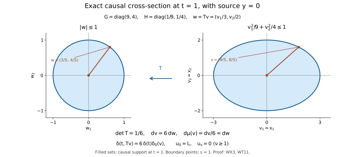
An anisotropic metric changes the delta weight. In two dimensions take and . Then The leading amplitude is one and all later ones vanish. The kernel has point-source coefficient , because the linear map to isotropic coordinates has determinant . Its convolution with has the unit initial-velocity normalization. Its spatial support at fixed is an ellipse, not a Euclidean ball of radius .
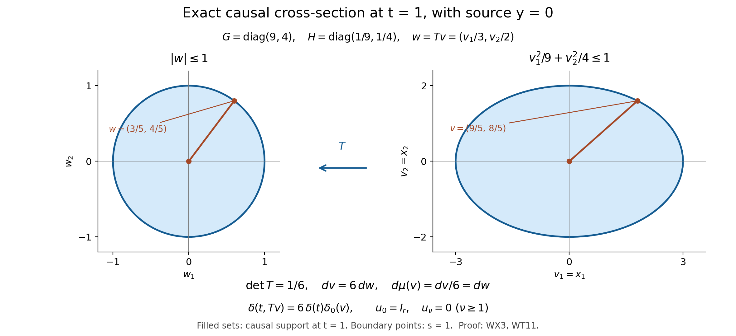
The figure uses the original example , , , and the exact map . The marked boundary points are and , both of distance one; the full coordinate Jacobian is six. The density and point-source factors are those proved in (WT11) and (WG18). The filled ellipse is a support cross-section, not a plot of a finite value at its singular boundary. Reproducible script and vector figure.
A constant matrix potential keeps its order in the expansion. Let , with any fixed complex matrix . Then , , and (WG5) gives The formula follows by induction: the transport equation for a constant amplitude is . No diagonalization, real eigenvalues or positivity are used. If , the finite sum with is already an exact causal fundamental kernel, since the displayed remainder vanishes.
13.1. A complete consequence for every constant complex potential
The nilpotent example has a further consequence at its original matrix generality. For any constant complex -by- matrix , every spatial dimension , and the original operator , the full original sum converges as a causal spacetime distribution, and on positive time with all one-sided derivatives into tempered spatial distributions. It is an exact fundamental kernel, with zero initial value and first derivative . This extends the finite nilpotent calculation; it is not an assertion that an infinite geometric Hadamard series converges for variable coefficients.
To prove it, retain the simplex formula (W22). Its nonnegative weight has integral (W23), and each derivative of of order is bounded on the real line by . For , the full product rule therefore gives, for every , For the derivative on the power , keep its falling product and its remaining nonnegative power; only orders through can occur. The other derivatives have at most labeled product assignments, each with its actual factors . Since , their absolute integrals are bounded by the original weight integral (W23). The finite binomial sum of the two derivative types is bounded by the displayed polynomial in , with a constant depending only on . This proves (WK2), including and ; the two factorial factors from the original amplitude and original are displayed before their numerical comparison.
The sum of the coefficients on the right converges: after their exact factorial cancellation, its successive ratio tends to zero, because the denominator contributes and its numerator has only the fixed polynomial ratio and . Pairing the retained polynomial frequency bound against any Schwartz test proves uniform convergence with every fixed time derivative, uniformly over bounded sets of Schwartz tests. The fundamental theorem and the same convergent bounds justify differentiation of the sum. Integrating such a pairing against a compact spacetime test, with its spatial Schwartz seminorms uniformly bounded in time, proves convergence as a spacetime distribution. Every partial sum is supported in ; testing outside that closed cone and passing to the limit proves the same support for the sum.
For the partial sum through , (WX4) gives its full error Its tested absolute bound is the right side of (WK2) at , with replaced by , and tends to zero on every compact time interval. Differential operators are continuous on distributions by their transposed test seminorms, so the complete finite identities pass to The uniform derivative convergence and (W19) give both initial data. On positive time the point source vanishes, so repeated use of the original differential equation gives every further jet, retaining its entire binomial expansion: Here , and the matrix power is the original identity. Scalar spatial derivatives commute with the constant , which proves that expansion; no commutation of variable matrix coefficients is inferred.
These data determine the evolution in the class of twice continuously differentiable tempered-distribution-valued solutions. Indeed Fourier transformation gives the original matrix polynomial . For a solution difference with zero initial data and a terminal time , choose a smooth compact frequency test . The backward matrix equation , with , has a smooth compactly supported test solution: the ordered finite-dimensional flow theorem NF6–NF11 applies on the compact frequency support, with all parameter derivatives, and the initial test factor keeps that same support. The exact bilinear distribution pairing has constant Wronskian Its initial value is zero and its terminal value is , so . Transpose is used because this is the bilinear distribution pairing; introducing a conjugate would change that convention. Arbitrary and arbitrary compact tests prove uniqueness. Schwartz continuity then gives uniqueness as tempered distributions too.
The smaller finite-order odd receiver from (WT12) also propagates to this exact sum. Define . Choose one integer with ; it satisfies (OE18) for every index. The finitely many indices with have the bounds already proved. For all larger indices, (OE8) and (OE15) give, on tests supported in with , These estimates are uniform in on compact sets; tests outside the cone simply pair to zero. Multiplication by the original amplitude norm gives a summable majorant, whose successive ratio has the two growing factors and in its denominator. The finite low-index bounds and this uniform tail prove weak continuity of into order when , and of its time derivative into order . For both valid bounds are order zero. The entire series agrees off the center with the spacetime odd difference by its tested convergence and agrees at the center by that continuity. In odd spatial dimension , choosing makes the primitive bound sharp: the zeroth term has a nonzero coefficient by (OE19), while every subsequent exceptional term has lower derivative order and the remaining tail has order zero. The scaled test used after (WT12) makes the leading term grow as and all those lower-order terms stay bounded. This sharpness assertion concerns positive rank; rank zero has the empty kernel. The source factors and all higher-index contributions remain in (WK1).
14. Problems and complete solutions
Problem 1 — The first three initial traces in one dimension. Compute for , integrate it against a smooth spatial test, and verify the first nonzero initial derivative.
Solution. Here , , so . At , substitution gives The odd Taylor term integrates to zero, and the remainder bound follows from the second derivative of on a fixed compact interval. Smoothness in follows by differentiating the fixed integral. Derivatives of orders zero, one and two vanish at zero; the third derivative is . Thus the trace is , with the exact normalization.
Problem 2 — Why the test order cannot be lowered. At , find , and show that a uniform order-three estimate cannot hold near .
Solution. Now , , and (OE19) gives Indeed and . If an order-three estimate uniform near held, continuity on smooth tests would pass that estimate to . Choose with , and let . Its derivatives through order three stay bounded on one fixed support, but the pairing with (WP2) grows as . This contradiction proves the claim.
Problem 3 — Weak convergence is not norm convergence. For , compute its distance from in total variation and its limit against a continuous test.
Solution. For , the three support points are distinct. The signed difference has masses , so its total variation is . On a continuous test , its value is , which tends to zero by continuity at the origin. These facts hold even on a fixed interval containing all points for small . They explain precisely why the topology in Section 6 was specified on fixed tests.
Problem 4 — Design an error with three continuous derivatives. In spatial dimension , choose the smallest truncation index guaranteed by this lesson to give a remainder for arbitrary smooth coefficients. Explain what fails at the next smaller index.
Solution. Inequality (WG14) reads , hence the smallest integer is . For , the exponent of the cone power is . At a nonzero cone point its third transverse derivative is a nonzero constant times and is unbounded. If , (WX4) makes the remainder amplitude a nonzero constant, so this failure actually occurs. At , , and Section 11 controls the cone and its vertex.
Problem 5 — A nilpotent system with an exact finite answer. Let Find a causal fundamental kernel and its first initial traces.
Solution. Matrix multiplication gives , every other entry of zero, and . Formula (WX4) with therefore yields Its causal support follows term by term, and the exact equation is . From (W19), and . Terms with start at orders three and five; they do not alter those initial data. This system is not diagonalizable, so an argument requiring diagonalization would miss it.
Problem 6 — A cutoff and the first affected time. A smooth function equals one where , and its derivatives are supported where inside a larger normal neighborhood. Show that multiplying every amplitude by changes no finite wave identity on . Determine whether the same conclusion necessarily holds at .
Solution. Each commutator term from contains a derivative of multiplied by a smooth coefficient, an amplitude, and a spatial derivative of . Distributional derivatives have support contained in that of , namely . At every point with , a neighborhood still satisfies ; therefore each such term is zero there. The difference from the uncut product is zero by the same argument.
Under the stated stronger hypothesis the answer at is also yes, locally near each point of that time slice. At , the closed support of each derivative of is absent from a neighborhood, because that support lies in the open set . Hence is locally constant there, and its value is one by continuity from . At it is already one, while at causal support makes the kernel vanish near . These three cases prove the local assertion. A single larger time interval would require a uniform positive gap between the affected region and ; it is not implied just by local separation over a noncompact set. The basic extension theorem in Section 11 uses only the open time interval and needs no such gap.
15. Exact comparison with the freely available author version
The comparison here uses Christian Bär, Nicolas Ginoux and Frank Pfäffle’s original author TeX for arXiv:0806.1036v1, §1.2, §1.4 and §§2.1–2.3, and the finite identity (2.13) in §2.4. It imports no global existence result, infinite-series assertion or proof from a printed edition. All distribution, transport and finite cancellation statements receiving this comparison have their proofs in this lesson and the precise earlier programme proofs already named.
Write for their spacetime dimension, and for their parameter. Their flat coefficient becomes Their quadratic form is the original . The future orientation is increasing , and their name for that branch is “advanced.” Their continuous starting range is , hence . Our original integral range in (W6) is broader, ; the full formulas agree on their intersection. Their definition of the remaining parameters applies the same wave operator recursively, so the compatible continuation (W10), tested on every compact smooth function, proves equality for every parameter, including the point source and exceptional dimensions. It gives the flat correspondence stated in the references, without replacing any coefficient.
For the geometric comparison keep the product Lorentzian metric Its complete Christoffel expression has zero coefficients whenever a time index occurs, since the time coefficient is constant, the mixed entries vanish and the spatial coefficients are independent of time. Its geodesics therefore have affine time and the original spatial -geodesic. The exponential map at is . Its tangent-volume coordinates have the original determinant , so its volume distortion is In particular the distortion is one at the center. The source definition in §1.4 pairs the flat Riesz distribution with the pulled-back test multiplied by this distortion. The full inverse test Jacobian of (WG6), followed by the normal chart, consequently gives the exact functional comparison The equality follows directly from their definition, not from their global theorem: retains every factor in the test substitution. It is first the equality of the original integrals and then the equality of their entire tested continuations. Here the domain is the actual common small exponential image, and tests have compact support inside it. No pullback by distance at the diagonal occurs.
The matrix lower-order terms also have an exact comparison. Put The last product acts on the section to its right; every derivative acts on both its coefficient and its section. Its first-order contribution is the original scalar volume drift and the matrix contribution , whose sum is . Its zeroth-order contribution is the negative of the two added terms in . Expanding proves the full operator equality in (WC5), with no commutation of matrices assumed. This is the connection-d’Alembert convention of their §1.5.
Let be the ordered parallel matrix along , with initial value . Its equation is , and its full solution and inverse are constructed by (WT5). The covariant form of (WT1) is . It gives Differentiate (WC3), and retain its two varying logarithmic terms. The term in (WC6) cancels exactly that term in the derivative of . The remaining equation is The proved uniqueness of (WG4) therefore identifies their zeroth coefficient with the exact .
Their source-point variable is our , and their receiving variable is our ; keep that order. Their radial recursion, at the original TeX labels vaunull and vaukaglatt in §2.2 and repeated in §2.3, has factor in front of its ordered integral. Substitute , retain and its inverse, and keep the time-independent operator on the coefficient. The time derivative is zero there. The exact result is Starting from (WC7) proves this for every index. With (WC4), their is consequently our integrated against the full density . A differential operator on this density representation has the exact coordinate functional action : pairing by the formal transpose verifies that multiplication by intertwines it with our coordinate-volume action. Multiplying (WG17) by changes its point coefficient to , while retaining its entire error . Thus their finite identity (2.13), with truncation index , is exactly (WG17) in this density representation. Every factorial, volume factor, operator term and source/receiver order is accounted for. This bounded author-version comparison claims no global Cauchy evolution and no convergence of an infinite Hadamard series.
References
This lesson obtains the causal constants from a Laplace integral and the time traces from a Volterra simplex, then treats finite-order restriction and geometric cancellation separately. The domain reconciliation in Section 7 is explicit because a negative factorial or a negative derivative order cannot be inserted into an endpoint expression outside its domain.
Christian Bär, Nicolas Ginoux and Frank Pfäffle, Wave Equations on Lorentzian Manifolds and Quantization, arXiv:0806.1036v1, §§1.2 and 2.1–2.4, compares Lorentzian Riesz distributions and bundle Hadamard coefficients. Their dimension is spacetime dimension, here, and their parameter is . They call the future-supported branch “advanced”; our causal kernel satisfies in their flat notation. Proposition 2.3.1 covers normally hyperbolic bundle operators, and their finite-sum identity (2.13) checks the cancellation. The finite-order restriction, vertex coefficient, and flat cosine normalization required here are proved explicitly above.
Further questions
Three directions continue the work. Quantitative coefficient dependence: for a fixed compact center set and a prescribed error norm, derive the finite list of coefficient seminorms needed in the transport and coordinate estimates. The proof supplies bounds but does not optimize that list. From finite parametrices to evolution: combine increasing-order causal errors with a suitable local solution operator to obtain an exact evolution and compare the resulting kernel with the flat cosine spectral relation. Such a step requires an existence and uniqueness theorem at the selected coefficient regularity; the finite identity alone is insufficient. Reflection at a boundary: construct the reflected exponential map and the boundary matching amplitudes before imposing Dirichlet or other boundary data. A cutoff of an interior normal kernel supplies neither the reflected ray nor a boundary condition.