Positive energy and vanishing at the far end of space
Decay at infinity can be tested by weights that grow as increasingly high powers of the radius. For a positive-energy equation, the useful estimate must control two scales at once: the power in the weight and the radius at which the solution is being tested. Their competition creates a characteristic frequency shell. An estimate that ignores that shell loses the second derivatives needed to handle rough leading coefficients.
We organize the argument around two complementary estimates. A Fourier calculation, localized on the sphere, recovers derivatives with carefully chosen radius-dependent coefficients. A difference of squared norms supplies the angular and positive-energy terms. Neither estimate closes by itself. Their combination makes the coefficient errors small and gives a weighted uniqueness theorem for complex Lipschitz perturbations of a real elliptic quadratic operator.
1. The exterior equation and its precise assumptions
Let , , be a connected open neighborhood of infinity: for some . Let The coefficients may be complex. They are locally Lipschitz on , and their symmetric part is elliptic on : Assume that for some , some , and all sufficiently large , The two powers in (E3) are distinct. No second derivative of a leading coefficient is assumed. Retain the full matrix, including its skew part. Put and . The exact comparison is Both derivatives remain to the right of the coefficient. Thus no derivative of a skew coefficient is introduced. Formula (E2a) proves that contribution is zero; it does not erase the original entries from the coefficient data.
Here is the complete formulation for an original real limiting matrix , which need not be symmetric. Replace the first assumption in (E3) by Assume its real symmetric part is definite. Choose its actual sign , and set The original remain fixed. The auxiliary limit is the full , with every skew entry retained. The theorem below holds in this formulation when . For the identity limit, , , and .
We prove every map needed to apply the exterior argument. The chain rule and its inverse give The derivative identity holds almost everywhere. Constant linear pullback and its inverse map bijectively to , : every weak derivative is the finite chain-rule sum, and changing variables contributes to its squared norm. Smooth approximation proves these identities at weak regularity. The distributional identity in (E3c) then follows for the weak Lipschitz coefficient product as well; it agrees with the usual expression when the local regularity has reached .
Let and be the smallest and largest singular values of . Then and . Assumption (E3a) and the full sums in (E3c) imply, entry by entry, The image domain contains . For the original inequality (E5), its complete pullback is In particular it has the required bound with the explicit additional constant . The original form of (E3e) is retained when returning the estimate to .
Put and . For every real exponent , The bounds on , together with (E3f), prove both directions of the all-weight condition (E4), including negative exponents. Ellipticity is also preserved exactly: the auxiliary symbol at a real covector is , and for . Equations (E2a) and (E8a) below account for the entire skew operator. Sections 2–12 prove the estimate for the auxiliary expression with these original data present, and (E77)–(E80) return it with its full Jacobian to the original operator. A negative-definite limiting form requires the original , since the positive potential is . The example in Section 13 shows why that sign cannot be omitted.
Exterior uniqueness theorem. Suppose , , and Suppose the distribution has a locally square-integrable representative away from the origin and satisfies Then almost everywhere on .
The same conclusion holds if the estimate (E5) is imposed only near infinity and is assumed on each compact subset of . The exterior proof uses (E5); propagation through bounded regions uses that local inequality. This more local sufficient formulation does not assert one global constant in bounded regions approaching a finite boundary of . If the displayed equation is imposed on all of , (E5) already supplies the local inequality on every such compact set. A value at the single point zero has no effect on an function as an almost-everywhere equivalence class.
Ellipticity on the whole continuation domain is explicit in (E2). The decay assumptions alone guarantee it sufficiently far out, since there. They give no ellipticity guarantee in an arbitrary bounded part added to . If only the exterior conditions are known, the conclusion proved below is vanishing on a sufficiently distant exterior region; the extension across a larger connected domain requires (E2) and the local equation there. This makes explicit the elliptic setting of the antecedent theorem.
The following prerequisites specify the current proof boundary.
- Fourier inversion and Plancherel. Sections 1–2 of Fourier transforms, finite spectra and convex separation supply the Fourier convention and Plancherel identity. We prove the parameter inequality used here.
- Weak elliptic regularity. Sections 7–8 of Local inverses and distance-weighted elliptic estimates define weak products with locally Lipschitz coefficients and give under second-order ellipticity. Section 6 of Local inverses and distance-weighted elliptic estimates supplies the interior estimate with constants uniform under a common ellipticity bound and coefficient modulus of continuity. Its application on large annuli is proved below.
- Derivative exchange. Section 4 of Curved weights and the directions in which support can end gives the finite integration-by-parts identity which exchanges derivatives across one Lipschitz multiplier. The total order drops by one; individual orders remain at most the larger original order. Its unequal-order refinement is available, but the non-strict version suffices here. The sphere adaptation is detailed in Section 3.
- Polar geometry. Section 3 of Detecting a solution from infinite-order silence at one point establishes the polar vector fields, surface measure, and their adjoints. We state the identities used here and rederive the exterior change of variable.
- Entry tools. Finite-dimensional compactness, real spectral decomposition, positive-definite matrix square roots, smooth coordinate charts, finite smooth partitions on the compact sphere, smooth cutoffs on intervals, the weak chain rule, and density in local integer Sobolev spaces are entry assumptions.
- Support normals. Section 7 of Curved weights and the directions in which support can end gives support-normal exclusion for locally Lipschitz elliptic principal parts at the initial regularity; Section 8 of Curved weights and the directions in which support can end gives the quadratic root-count argument. We verify its applicability to a complex coefficient field approaching the identity, without assuming that the coefficients become real at a finite point.
We use the stated predecessor results and prove the exterior estimate below.
For the proof choose once and for all The original condition (E3) implies the same bounds with in place of when . Thus using in an estimate imposes no extra restriction on the theorem. The number controls the curvature of the weight. All constants may depend on these two fixed numbers and on , but never on the subsequently large parameters and .
2. A cylindrical operator with a growing potential
Set , , and . Write for the projection of onto the tangent space of the unit sphere. The identities in Section 3 of Detecting a solution from infinite-order silence at one point are The last two formulas use surface measure. Individual are not skew adjoint. Their divergence corrections cancel in the sum of squares because .
Twice applying the first identity, with the derivative of retained, gives There is no derivative of in this formula: (E1) has coefficients to the left of the derivatives. When , expand (E8) and use (E7) to obtain For the full comparison (E3b), apply this calculation to and , so the original point is . Write , retaining each of its three contributions. The exact frozen skew contribution is The equality follows from twice applying the full polar formula (E7). Pairing indices in the last sum proves zero because the second derivatives commute and is skew. The surviving expression is (E9) plus every term from ; (E3d) gives its two required decay bounds. In all subsequent formulas for this case, , the coefficient error comes from the complete , and the positive potential uses . No original matrix entry or sign has been silently replaced.
Every other coefficient in this cylindrical expression, together with its first cylindrical derivatives, is . An angular or derivative of introduces one factor , exactly balancing one power in the derivative bound of (E3). Derivatives of the smooth sphere factors are bounded.
Now introduce the increasing coordinate For , , and and are uniformly bounded. Put . Multiply the operator in (E8), with the term added, by . It becomes where Here denotes a fixed ordered word; we may sum over all words of the specified length. Indeed , with , which proves the formula for . Smooth factors involving preserve the last bound of (E12), including its weak first derivatives.
The potential is retained as a main term. Direct differentiation gives after increasing a fixed lower threshold for . The sign is used here.
In these coordinates the differential inequality becomes To check the powers, before changing , multiplication of (E5) by gives a zeroth-order term and first-order terms . The bounded factors in (E10) then give (E14). The norm convention on the cylinder is ; it is not Euclidean measure. The latter is
For , write Thus every in (E11) is replaced by , whereas angular derivatives are unchanged. Our target is for compactly supported smooth in . Since is comparable to , this is also the estimate with weight on each derivative of order .
3. The error budget and one-derivative algebra
Let denote the finite family of all words of length in . A squared norm of this family means the sum of the squared norms of its members; . On a fixed sphere chart these norms through order two are equivalent to coordinate Sobolev norms, with lower orders included. Define The highest-order term uses exactly order two; it carries both and . We will not replace it by an unweighted lower-order error.
Two elementary product estimates explain this choice. Consider a term All the indices here are nonnegative integers. If , then , and the integrand is the product The square of the second factor is bounded by the order- term in the decaying part of , because . Cauchy–Schwarz and bound (E19) by . The case is identical with the two factors reversed. If , use , hence for , and . The product of and dominates the integrand. Their squares again occur in . This proves a uniform bound for every monomial in (E19), not just a representative highest-order term.
We also need products containing the potential. If and its first derivatives are , then Consequently, for every fixed , For the first integrand apply Young’s inequality to and ; for the second use and . The factors give the displayed right side. Constants in (E21) may contain the fixed energy .
Here is the exact algebra allowing only first coefficient derivatives. In a Euclidean chart, for , the difference is a finite sum with multiplier , total derivative order , and each individual order no greater than . This is the derivative-exchange result in Section 4 of Curved weights and the directions in which support can end. It follows by transferring an unmatched derivative once; when the two factors have equal orders, interchange one derivative from each factor before continuing. Each transfer differentiates once in its own integral. One never differentiates that error again.
For a sphere chart with smooth density , replace by . Its derivative is , so the estimate contains both and , with bounded chart constants. Expanding a word of sphere fields into coordinate derivatives produces its leading coordinate monomials and lower-order terms with bounded smooth coefficients. Reordering two sphere fields costs their commutator, a smooth first-order field. These costs also lower the total derivative count by one. The finite atlas has uniform bounds on these smooth factors.
For later use, attach degree one both to and to each derivative. A differential polynomial of degree at most two and its formal complex conjugate have equal squared principal symbols. Expanding their squared norms, pairing terms with indices and , and using (E23) therefore removes every term of total degree four without differentiating a coefficient twice. The remaining terms have the form (E19). If one factor was multiplication by , the degree-two exchange leaves at most one derivative on , or one power of and no derivative, and (E21) gives exactly (E22). Terms of degree below two already satisfy the same counts. This proves the assertion for every pair of monomials; linearity and the finite number of monomials prove it for their sums.
In this argument “formal complex conjugate” is an algebraic operation on the displayed polynomial, not the assertion that the resulting operator is the Hilbert adjoint. We never expand the actual adjoint of a rough second-order monomial: doing so could introduce distributional second derivatives of its coefficient. Instead each paired integral exchange differentiates its combined multiplier once. Reversing the order of smooth sphere fields and using their divergence corrections costs only the lower-degree geometric terms described above. This distinction is essential for Lipschitz coefficients.
4. A Fourier inequality across a characteristic shell
Let , , , , and Assume the four conditions Then, for , The constant depends only on dimension. The same proof works in dimension one, with the angular sum empty.
Proof. Put and The Fourier symbol of is , so its modulus is . The finite monomial sums on the left of (E25) are comparable, with dimensional constants, to It suffices to bound this by .
First suppose On this set . For completeness, divide by and put . For , the real part bounds a fixed multiple of . On , the closed subset (E27) is compact and contains no zero of : such a zero has and , excluded by (E27). Its modulus therefore has a positive minimum. These two regions prove the claimed uniform bound. The first condition in (E24), multiplied by , controls by . Since , its first term is bounded by , and hence by . Finally This proves the bound away from the shell.
On the complementary set, , , and . Thus . The second condition in (E24), multiplied by , controls by . The angular term already controls . The last condition gives Every term in (E26) is now bounded. The two sets may share their boundaries; the constants are uniform there. Multiply the pointwise inequality by , integrate, and apply Plancherel. Its fixed normalization factor cancels from both sides. This proves (E25).
5. Choosing the radius-dependent coefficient
The potential in (E11) is of size on a slab where . To place its square in the term of (E25), we also require An admissible choice, of the smallest order allowed by the lower bounds, is Both formulas agree at each transition. This is an optimization up to absolute constants, not a claim of an exact unique minimizer.
Here are all the checks. In the first region , so the first two conditions in (E24) hold, and (E30) follows from . In the middle region , while ; the first two conditions again hold. Moreover since . In the last region and ; also , proving both conditions.
In these three regions, respectively, Therefore the remaining two conditions in (E24) hold whenever The inequality also holds in every region. In the first, and hence . In the middle, , giving . In the last, , giving .
For the eventual estimate set This has and . On a slab meeting , one has . Since , increasing the fixed threshold for ensures Thus (E33) holds uniformly for every slab. Also when both and are sufficiently large. There is no factor in the exponent in (E34).
To verify the asserted scale optimality, the second condition in (E24) and (E30) imply When , the second term is between and , and dominates the first up to constants. When , it is between and ; comparison with divides this range at . This proves that (E31) is within a factor two of the necessary lower bound.
6. Derivative recovery in one chart and one slab
Rotate the sphere to center a chart at its north pole and use with . The last coordinate is . The induced metric and its inverse give For example, the density is the square root of the determinant of , and the inverse matrix is . Substituting these into the divergence formula for the Laplace–Beltrami operator gives the middle identity. Thus the coordinate gradient norm and the angular gradient norm are comparable with fixed constants on a fixed small chart. The same is true through order two after adding lower orders, by expanding each field and expressing each coordinate derivative in the spanning fields.
Suppose is supported in this chart and in , . In these coordinates write The polynomial has total degree at most two in derivatives and , with coefficients bounded by . It includes the variable principal coefficients and all their conjugated -terms. The polynomial has total degree at most one, with uniformly bounded coefficients; it includes and the bounded first-order sphere terms. To see these bounds directly, subtract the leading constant matrix in (E36), use , and use (E12). No derivative of a rough coefficient is used in this step.
Put in the coordinate chart. Expanding the finite polynomials in (E37) gives Use (E25) and . Choose the fixed chart radius small first, then choose fixed sufficiently large lower thresholds for and , so the contributions (E38) consume at most half of . The equivalence of the smooth density norms changes only fixed constants. The potential contributes where (E30) is used. This is a bound by the designated potential term on the right, with no smallness assertion about .
On the slab, powers of and are comparable by constants determined by its fixed width. After (E38) has been absorbed, one may drop the factors in the retained first sum. We obtain The first sum here deliberately has no remaining powers of . Its stronger predecessor was needed for the coefficient absorption; (E40) alone would not justify that absorption.
Now use (E31) and (E34). The inequality gives . The third condition in (E24) gives where is used in the second step. Retain this lower bound only for order two in (E40), and keep the displayed -weighted lower orders. It follows that This proves the required derivative estimate on each chart and slab, with constants independent of their location.
7. Localization with constants independent of support
We now prove (E42) for every . Choose finitely many real smooth functions , supported in charts of the fixed size used above, with . Such a square partition is obtained from any nonnegative subordinate partition by dividing its members by the square root of the sum of their squares. The denominator is smooth and strictly positive on the compact sphere.
Choose a real nonnegative smooth function supported in , positive on . Normalize it by the square root of the sum of the squares of its integer translates. The result is a smooth , with , such that The denominator is smooth, periodic, and bounded away from zero. All derivatives of of any fixed order are bounded uniformly in . Put Only a bounded number of these functions meet a point. A slab meeting has , so (E34) is admissible with , including slabs whose lower endpoint is below . The function itself still has compact support above .
Apply (E42) to these functions and sum. Zeroth-order terms sum exactly. For each real field in , expansion and give For order two, the product rule shows that equals minus terms bounded by on the cutoff support. Squaring, summing, and using bounded overlap yields The last term is absorbed into after increasing the parameter thresholds. Thus the summed left sides control , up to fixed constants.
The growing potential commutes with all cutoffs. In the other terms of , two derivatives may hit , or one may hit and one may remain on . Conjugation supplies at most one in a nonzero commutator, since a term is multiplication. Explicitly, and . Coefficients stay on the left and are uniformly bounded; none is differentiated. It follows that The angular right-side terms in (E42) contribute, besides a fixed multiple of the original angular norm, at most . The potential norm sums exactly. Therefore the only additional right-side errors are . They are absorbed by for large thresholds, since . This proves the global estimate (E42). The number of slabs occupied by never enters its constant.
8. A norm identity revealing the two positive terms
For the moment set in (E11). Define Then , and its algebraically reversed companion is . With respect to , and . Hence The real part makes this identity independent of which slot of the complex inner product is chosen linear.
We compute it completely. Since , These derivatives concern the smooth scalar functions , not a rough principal coefficient. Insert (E48) in (E47). Integration by parts in combines into ; the angular integration uses (E7). Thus the exact identity is This identity is also a useful sign check on the direction of the curved radial adjustment.
Let . We have , , and . Therefore for sufficiently large , uniformly for large . The first term in (E49) is bounded below by . The part is bounded below by , so both of these costs lie in . By (E13), and by enlarging if needed, For example for large , while , which is absorbed in the excess above . Combining (E49)–(E51) gives The reserve will pay for the coefficient-potential products.
9. Restoring complex Lipschitz coefficients
Let be the conjugate of in (E11). Define The order of each displayed word is preserved. This reversal is well defined for locally Lipschitz coefficients because it does not differentiate them. It is not identified with .
Subtract the background difference (E47) from . We examine every type of resulting product.
Products with the potential. The terms are For a second-order monomial the terms without a derivative on its coefficient cancel after one exchange of derivatives. The remaining integrals have one derivative on and at most one derivative on . A first-order monomial leaves a zeroth-order product; its conjugation can contribute one . For a zeroth-order monomial the real parts cancel without integration, including the term with two powers of produced by conjugating a radial second derivative. Indeed since is real. Thus no term remains in this class. The same statements follow for angular words by the density and adjoint calculation in Section 3. Thus the total absolute value is bounded by Here (E21)–(E22) were used. For sufficiently large , the first term is at most the potential reserve in (E52), while the rest lies in .
Products with one perturbation coefficient and no potential. Expand the powers in , and the corresponding reversed powers in . Each term has degree at most two. All products of total degree four cancel at principal-symbol level by the exchange identity (E23). Terms left by that exchange have degree at most three, individual derivative orders at most two, and a multiplier bounded by . The multiplier is a product of one perturbation coefficient with smooth background factors or its first derivative; all such quantities satisfy this bound by (E12). Commutators of sphere fields and their divergence corrections also have this bound and lower the differential order by one. Every resulting integral is therefore one of the finitely many types (E19), and is bounded by by (E20) and its lower-order case.
One can check the cancellation directly in coordinate -notation. Write the leading polynomial as . Its reversed partner has the conjugate leading coefficients. In the difference of the two squared norms, swap the two coefficient indices in the second sum. The coefficient of the derivative product is then the same in both sums, leaving exactly the antisymmetric combination (E23). Each application of (E23) consumes one derivative, leaving . Lower-degree pieces that arise when an ordered field word is expanded already have this loss. This also shows why the individual order may remain two.
Products with two perturbation coefficients. Apply the same paired expansion to . A multiplier is now a product of two perturbation coefficients; it and its first derivatives are . For this is bounded by . The same exchange removes the total-degree-four terms, and all remaining products again satisfy (E19). Their contribution is bounded by .
The three classes exhaust the squared-norm expansion. At no point is a differentiated coefficient differentiated again: the exchange identity is applied to each original multiplier, and its error integral is bounded immediately. Combining these bounds with (E52) proves The initial calculation uses smooth and Lipschitz coefficients. Weak integration by parts justifies the coefficient exchanges directly. Equivalently, one can first smooth the coefficients on a compact neighborhood, use their uniform Lipschitz bounds in the finite formulas, and pass to the limit without introducing any second-derivative coefficient bound.
10. Recovering the longitudinal energy
The radial derivative does not occur with a useful sign in (E55), so we recover it from the difference of the operators. Equations (E46) and (E53) give By direct expansion of these finite polynomials, Since uniformly, the triangle inequality and the square of a finite sum imply Divide by . For , the error is at most . For , it is at most the corresponding decaying term . Thus the divided error is bounded by . Equation (E55) also gives . Insert this in the divided version of (E58), and add the positive terms from (E55), decreasing their fixed coefficients if necessary. We obtain The division by in this argument is what puts the second-derivative perturbation into the exact remainder (E18).
11. Closing the two estimates in a fixed order
Put , and retain the entire from (E59), including the radial term. The global form of (E42) says where is a fixed constant large enough to include and .
Let . Since , it tends to zero as . For , . The zeroth-order decaying part of is therefore at most . Its first-order angular part is bounded by . The radial part obeys Consequently This is the step at which discarding the radial term in (E59) would leave an error uncontrolled.
From (E60), both and . Substitution into (E61) yields Choose sufficiently large, then a sufficiently large lower threshold for . Because , these choices make the coefficient of in times (E62) at most , and the coefficient of at most one. All earlier thresholds can be included by taking their maximum. Equation (E59) then gives Substitute (E63) back into (E60): . The potential term in gives . Together these prove (E17). The constants work for every and above the chosen fixed thresholds.
Finally, undo the conjugation. Angular fields commute with , and Thus (E17) implies In fact the two displayed left sides are equal. For compactly supported , integration of gives because the real part of is zero. Together with the unchanged angular and potential norms, this proves the equivalence of (E17) and (E64); using in place of only changes fixed constants. The estimate (E64) extends to compactly supported functions inside the cylinder. Approximate in on a fixed compact neighborhood of the support; the weights and coefficients are bounded there, and is continuous. The approximation is taken with fixed. No parameter-uniform smoothing assertion is required.
The estimate for the full original operator and measure
Retain the original data of (E3a)–(E3f). For an original point , put , , and let be the unique solution of . Its existence and smoothness for follow because the derivative is strictly positive and the function ranges from to . The actual fields in the original coordinates are For , the full chain rule gives and . Repeated application preserves every ordered word, including all derivatives of a field coefficient. The exact operator and measure identities are Indeed (E8) applied to the complete auxiliary matrix, with its energy , is multiplied by , which proves the first identity. The second retains both the original constant linear Jacobian and the radial Jacobian, followed by .
Set , large enough that lies in . Substituting both identities of (E78) into the proved estimate (E64), without deleting any measure or radial factor, gives for every original test function supported in this exterior region The constants are those already proved for the full auxiliary coefficient error, sign and positive energy. The original operator, energy, solution coordinates and measure are explicit on both sides.
To verify that every Cartesian derivative has a receiving map, put . Then The left field in the second identity acts on the whole bracket: it differentiates , , , and the original function wherever the product rule requires. This follows from (E7) and the full matrix chain rule (E3c). Conversely, (E77) gives every field in terms of original Cartesian derivatives. Iteration through order two supplies both complete finite derivative arrays, with their original radial and matrix factors. The all-weight correspondence (E3f) therefore transfers the weak solution, annular regularity and every cutoff limit of Section 12 in both directions. Its exterior zero region is the actual ellipsoidal region , and the original domain and local inequality then receive the proved continuation argument.
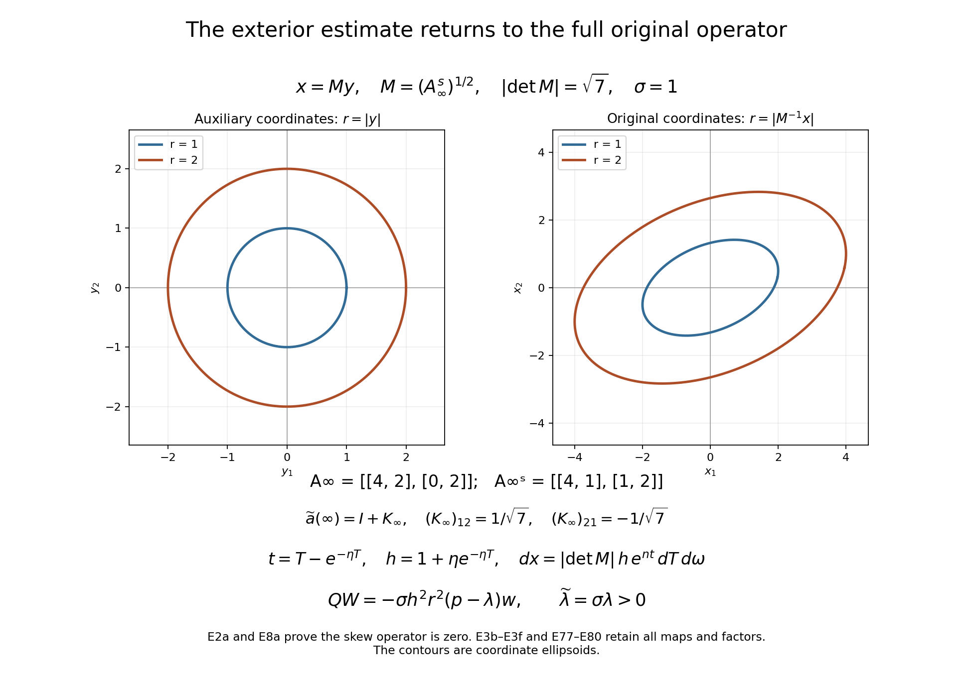
For the displayed example, , , and . The full auxiliary matrix is , with off-diagonal skew entries and . The contours are the original coordinate surfaces , rather than frequency surfaces. Equations (E3b)–(E3f) and (E77)–(E80) prove every map and factor in the diagram.
12. From weak decay to an actual open zero set
We prove the theorem of Section 1, beginning with the regularity needed to use (E64).
On every compact subset of , (E5) and give . Weak elliptic regularity in Sections 7–8 of Local inverses and distance-weighted elliptic estimates therefore gives . The initially weak product is It agrees with the usual nondivergence expression after this regularity improvement. In particular no second derivatives were assumed in (E4).
We need this improvement with weights at infinity. Let and . For sufficiently large , both lie in . Scale and write . The coefficients on the fixed annulus have uniform ellipticity and a common modulus of continuity. Indeed they approach the identity uniformly, and their first -derivatives are bounded by . The interior estimate in Section 6 of Local inverses and distance-weighted elliptic estimates, on a fixed pair of nested annuli, has a constant independent of . Scaling its version back yields The same statement with a harmless separate first-order term on the right would also suffice; it follows from the stated estimate by the interior interpolation inequality. The factor from scaling the norm occurs on both sides and cancels.
By (E5), For every , (E4) bounds the right side of (E66), and hence every term on the left of (E65), by . To see this directly, on the function is comparable to ; take in (E4). It follows by summing dyadic annuli, whose enlarged annuli have bounded overlap, that For a given , choose the annular exponent larger than ; the squared annular estimates then sum as a convergent geometric series.
Every cylindrical derivative through order two is a bounded sum of , . This follows by reversing (E7) for first derivatives and then applying it again; derivatives of the sphere factors are bounded. Using (E15), bounded, and (E67), we conclude For instance, the measure conversion for the -th Cartesian contribution changes a squared exponential weight into a fixed radial power comparable to ; (E67) allows every such power. This checks the Jacobian, rather than inferring (E68) from a pointwise assertion of decay.
Fix above the thresholds used in the Carleman estimate. Choose a real smooth cutoff , zero for and one for . Let be one for , zero for , with first two derivatives bounded independently of . Apply (E64), by its extension, to For a fixed , (E68) permits in every term. In detail, all upper-cutoff commutators are supported in and are bounded by , since the potential commutes and has bounded differential coefficients. Their weighted norms tend to zero by (E68). Equation (E14) makes square integrable, so the noncommutator terms converge as well. Derivatives on the left converge by the same argument. Thus (E64) holds for . Smoothing occurs first for each compactly supported , then at fixed , and only later will .
Write Using (E14), the product rule, and , we obtain Here is a fixed finite norm of on the transition strip , with any fixed bounded weight such as included. It is independent of . The constants controlling the equation near infinity are uniform in the strip position once the initial threshold is fixed.
By (E64) and (E70), Increase the fixed , then the lower threshold for , until . Absorb the first right-side term. For each fixed , restrict the zeroth-order norm to , where , to deduce Let . The right side tends to zero with fixed. Taking a countable union of these regions as proves for . We have obtained a nonempty exterior open zero set for .
It remains to justify continuation throughout . In dimensions greater than two, Section 8 of Curved weights and the directions in which support can end says that every real normal is admissible for every elliptic complex quadratic form. In dimension two, choose independent real covectors . The two roots of cannot cross the real axis as varies, by ellipticity, and their upper-half-plane count is locally constant. Far out, is positive definite. The path , , stays elliptic. At its roots are a nonreal conjugate pair, so the upper count is one also at . Connectedness of makes the same count equal to one everywhere. Thus a double nonreal root never occurs, and every real normal is admissible throughout . This argument uses asymptotic positivity; it does not assert that are real at some finite point.
On , the local equation has bounded lower-order coefficients on compact sets. Section 7 of Curved weights and the directions in which support can end therefore excludes every normal to a proper support boundary. Its open-set propagation consequence gives on this domain. When , removing one point from a connected open set leaves it connected: a polygonal path can be modified inside a sufficiently small ball about the removed point by an arc on a sphere, without leaving the open set. If , its singleton is a null set, so vanishing off zero proves the asserted almost-everywhere conclusion on .
For , a connected open neighborhood of both ends of the line is the whole line. Interpret as its two points, with counting measure; the angular fields and their sums are zero. The polar identity is , which is (E9) for . All estimates above remain valid on the two half-cylinders. The Fourier shell in Section 4 is empty in this case; its off-shell estimate suffices. The proof of (E52) used only boundedness of and , so also applies. The two exterior tails vanish. In dimension one a nonzero quadratic symbol has no exceptional nonzero normal, by Section 8 of Curved weights and the directions in which support can end. Propagate from the two tails on the two components of , and ignore the null singleton. The same reasoning proves a one-ended version on a half-line which avoids the origin; if a half-line crosses zero, propagation across it needs a locally bounded differential inequality there. The singular inequality (E5) alone does not supply that additional conclusion. This completes the theorem in every dimension.
12.1. Polynomial weights on one tail suffice for the solution alone
The proof of Section 12 uses weighted norms only on an exterior region. Its first-derivative assumption follows from an energy estimate there. We prove that implication without assuming global integrability near a finite boundary of the original domain.
Corollary. Retain (E1)–(E3), , , the inequality (E5) near infinity, and the locally bounded continuation inequality on compact subsets of . In place of (E4), it suffices to assume, for one exterior radius , Then the original solution vanishes almost everywhere on . The two-ended dimension-one formulation and the qualification for a half-line crossing zero remain exactly those in Section 12. For the full real definite limiting matrix (E3a), the same conclusion holds with the original required energy sign . No all-weight derivative assumption, or global integrability approaching a finite boundary of , is required.
Coercivity of the full complex matrix on a large annulus. Select so large that, for every , the closure of lies inside the region where (E3) and (E5) hold and inside . Increase to ensure . The entrywise bound gives . Indeed for a complex vector , each component of has absolute value at most the entry maximum times ; summing its component squares proves the displayed norm bound. Consequently This uses the full complex sesquilinear expression. Positivity on complex vectors has not been inferred merely from the real-covector ellipticity assumption.
The full annular energy identity. Choose a real smooth cutoff , with , equal to one on , compactly supported in , and put . Set , , and retain The coefficient follows by bounding each of the terms in each by , and then taking the Euclidean norm of its components. On the cutoff support, the original inequality and local regularity give . Sections 7–8 of Local inverses and distance-weighted elliptic estimates give on a neighborhood of that support. The weak integration identity can therefore be proved by approximation and the Lipschitz product rule. Its exact nondivergence form is All integrals are over the cutoff support, extended by zero outside it. The plus signs result from , with one integration by parts in . The original full skew entries, their derivative contribution to , and both cutoff terms remain in this identity.
Take real parts and use , (ECT2), Cauchy–Schwarz, and . The equation term is bounded by . The coefficient derivative term is bounded by . The cutoff cross term is bounded by . Thus The exact inequality follows by squaring . Since on , it yields Every term of decreases for . We therefore have the explicit common finite bound for the entire right coefficient. No weighted derivative assumption entered the proof.
Every weighted gradient tail follows. For , the ratio of the maximum of on to its minimum on is at most . For , use ; for , use . Both are in particular at most six, and the sign of determines which endpoint is the maximum. Multiplying (ECT6) by that maximum gives the full comparison Use , . The annuli cover up to their sphere boundaries, which have Lebesgue measure zero. For a given positive radius, membership in an enlarged annulus requires ; at most four integer indices meet this condition. All these enlarged annuli lie in . Summing nonnegative integrals therefore proves The right integral is finite by (ECT1) outside the larger of and . The intervening closed bounded annulus is compactly contained in , and its weight is bounded, so local supplies its finite integral. This is a local argument on a compact subset, not an assumption of integrability near an arbitrary finite boundary of .
Now (E65)–(E66) use only the original solution and first-derivative norms on those enlarged exterior annuli. They give every second-derivative tail weight (E67), and the full radial Jacobian gives every cylinder weight (E68). The entire cutoff argument (E69)–(E71) consequently applies, with its original order of limits, to obtain the same exterior open zero set. The root-count and compact-set continuation argument (E72), including its dimension-one qualifications, then gives almost everywhere on the original . This proves the corollary without invoking the preceding theorem under an unmet global version of (E4).
Returning a full definite limiting matrix. Keep every datum in (E3a)–(E3f). The exact auxiliary field is , with limit , rather than . Introduce its symmetric part for the energy estimate. Formulas (E2a) and (E8a), with the same weak product argument as (ECT4), prove on punctured compact sets. Its limit is exactly . The full entry and derivative comparisons in (E3d) give its two required decay bounds, since averaging a pair of entries retains those bounds with their displayed matrix sums. Apply (ECT2)–(ECT9) to this auxiliary symmetric field and positive energy , retaining the exact inequality (E3e).
The original solution tail (ECT1) transfers to by the actual singular-value inequalities in (E3f). Choose the auxiliary threshold large enough that exceeds every original coefficient, equation and domain threshold. For each exterior radius , the exact restricted measure and gradient identity is The inverse gradient entries and both singular-value weight constants in (E3f) show its finiteness after (ECT9). The region is contained in , so it supplies an actual original radial gradient tail as well. Sections 2–12 then return the exterior zero set through the complete maps (E77)–(E80). All original skew data, the sign , energy , gradient , integration regions and determinant remain explicit.
Equivalent tests for the weight quantifier. It is enough to test (ECT1) on any real sequence tending to , including the nonnegative integers. For a fixed real , select . Since , the exact inequality bounds the required squared integral by that tested one. Conversely all real weights include every selected sequence. This proves the equivalence for the original solution and, after (ECT9), its derivative tail, without changing their measures or domains.
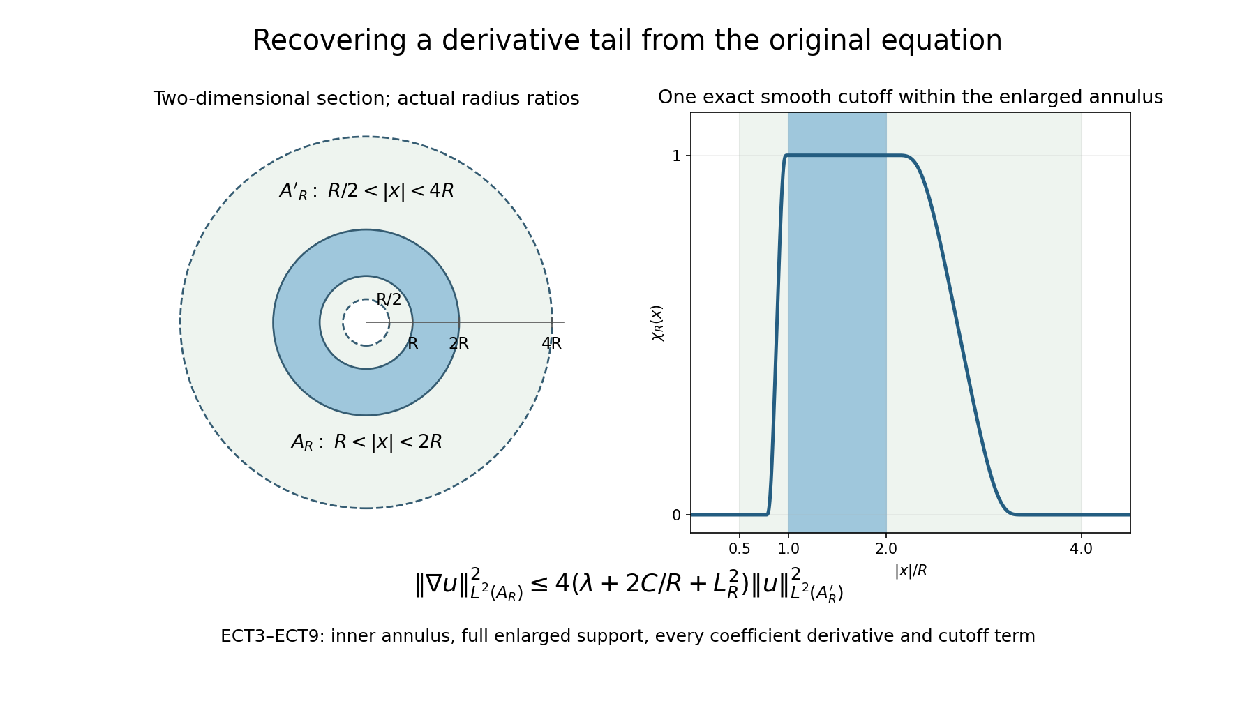
The drawing is a two-dimensional section of the -dimensional supports in (ECT3)–(ECT9), with all four radii in their actual ratio. Its displayed cutoff is the exact function The denominator is everywhere positive. Repeated derivatives of on the positive ray are a finite polynomial in times ; they all tend to zero at zero. Thus and are smooth, with on and on . This is zero for and , equals one for , and is smooth even at the origin because it vanishes in a neighborhood there. Its support is compactly contained in the enlarged annulus, and its smooth gradient has finite maximum . This verifies every cutoff property used in (ECT3) for the actual drawing.
This annular argument is a consequence of the complete exterior proof here. The original theorem and its solutions remain intact. In particular the outgoing wave (E75) still fails the required all-weight condition on the solution itself, and the negative-energy example (E74) still prevents deletion of the energy sign.
13. Worked models and precise nonconclusions
A complex angular perturbation at the allowed regularity. Let be a real symmetric matrix with Lipschitz entries on the sphere, and put, on , For real , , so ellipticity is immediate, independently of the size of . Radial differentiation of gives , and angular differentiation of introduces one factor . Thus (E3) holds almost everywhere. If measurable lower-order coefficients satisfy then every solution of at the stated weak regularity satisfies (E5). For , (E4) forces that solution to vanish. This example allows genuinely complex leading coefficients and merely Lipschitz angular dependence. It does not use a self-adjoint realization of the operator.
The sign of the energy changes the answer. In dimension three, set For a radial function , . Here so . Therefore with , and belong to every polynomially weighted space on the exterior. The function is nonzero. Equivalently, for the negative-definite symbol of , the same function solves at positive energy. Thus the relative sign cannot be discarded when comparing a general real elliptic limiting quadratic form with its auxiliary expression.
A polynomially weighted solution which does not satisfy all weights. Still in dimension three, let The same radial calculation, with , gives . Since and , both weighted integrals for and behave at infinity like . They are finite exactly when . This provides many weighted conditions, but not (E4); there is no contradiction with the theorem.
Small values do not control coefficient derivatives. Consider Its real part is the identity and its distance from satisfies the first bound in (E3). Its radial derivative contains , so the second bound in (E3) fails. The theorem has not been proved under only the first bound. This example identifies a missing assumption in an attempted application; it is not a counterexample to a more general uniqueness theorem.
These examples isolate four different issues: complex coefficients, the sign of the limiting form relative to the energy, quantification over all weights, and independent control of first coefficient derivatives.
14. Problems with complete solutions
Problem 1: anisotropy and the unchanged decay exponents. In , suppose the coefficient matrix tends to with the two rates in (E3). Find the full linear coordinate comparison, retain the original matrix and Jacobian, and determine the energy sign required by the theorem.
Solution. Put , so . The chain rule gives ; hence the new coefficient matrix is Its limit is . Since , the error is . Differentiating introduces only a fixed matrix factor, giving . The Jacobian is the constant . Formula (E3f), with , gives the exact weighted integral and both comparisons for every real exponent. Formula (E79) retains that factor six, every radial and factor, and the original in its original coordinates; (E80) supplies every original derivative. The spectral parameter is unchanged because the change of variables has not multiplied the equation by a scalar. Thus the required sign is . If the limit were , multiplication by would replace the energy by ; the theorem would require the original .
Problem 2: locate the three regimes without losing a parameter. Take , , and with . Compute the choice (E31), identify both transition exponents, and check .
Solution. For , the conditions and become and . When , one has , and all the expressions agree for every . For the regimes give At , the first two exponents are both one. At , the last two exponents are both . Every exponent is at least one in its designated range, proving . Moreover equals , , and , respectively. The middle exponent is at least , which checks the condition when .
Problem 3: why the second-derivative error has its stated weight. Bound by . Explain why replacing its first term by an unweighted norm does not follow from the same argument.
Solution. Factor the integrand as in (E20) and apply : Since , the second term is at most half the corresponding term in . The first term is exactly its order-two term. There is no pointwise or unrestricted norm inequality bounding two derivatives by one derivative. For example a fixed compactly supported amplitude multiplied by in a chart has second-derivative norm growing like , while its first-derivative norm grows like . The separate Fourier estimate, involving , is what eventually controls that order-two contribution.
Problem 4: a lower limit for the shell parameter. Assume (E24) and (E30). Prove the necessary lower bound (E35), and explain why cannot be used for in all three regions.
Solution. Rearranging the second inequality of (E24) gives ; (E30) gives . Their maximum is (E35). If and , then , violating (E30). If , then , violating the first inequality in (E24). Thus the middle expression fails in both sufficiently extreme regions, for two different reasons.
Problem 5: the endpoint cutoff limit and its order. Suppose only (E68) and (E14) are known, and are as in (E69). Show that the upper-cutoff error disappears for each fixed , and explain why this is not a uniform statement as .
Solution. Every derivative of is supported in , with a bound independent of . Since the coefficients of the differential part of are bounded, the product rule gives for . The right side tends to zero as a tail of a fixed function, by (E68). The potential contributes no commutator. Also by (E14) and the cases of (E68), so multiplication by converges on the equation term. Nothing in (E68) bounds the norms uniformly over all ; the constants may grow arbitrarily with . Therefore the justified order is smoothing on a fixed compact set, removing the upper cutoff at fixed , and then sending to infinity in the already established estimate.
Problem 6: propagation without a real coefficient point. Suppose , is connected, the quadratic principal forms are continuous and elliptic, and their real parts are positive definite at one point. Prove that every line polynomial (E72), with independent real , has one root in each open half-plane throughout . Explain the consequence for a locally Lipschitz equation which vanishes on an exterior open set.
Solution. At the selected point, the path that multiplies the imaginary part of the form by keeps its positive real part and hence remains elliptic. At , the real quadratic polynomial in the line parameter has no real roots and therefore has a conjugate pair. The upper-half-plane count is one. A root cannot cross the real axis along this path, so the same count holds for the original complex form at that point. For a fixed independent pair , continuity of the unordered two-root set, including multiplicities, follows from the quadratic formula. Ellipticity prevents real roots everywhere in , and the leading coefficient never vanishes. Consequently the upper count is locally constant and hence constant on connected . It remains one. The roots are distinct, since a double root would put both in one half-plane. The same argument applies to every independent pair; dependent pairs only give the zero complex vector excluded from the exceptional-normal definition. Thus the exceptional normal set is empty. Section 7 of Curved weights and the directions in which support can end then propagates any nonempty open zero set through a connected region where the lower-order inequality has locally bounded coefficients. The proof used a point with positive real part, not a point at which all coefficients were real.
References
The proof of the asymptotically constant operator is given here; it includes the parameter and subsidiary error estimates. The sign convention and the ellipticity needed for propagation have been made explicit.
For a comparison with scattering applications, Richard Melrose’s Spectral and scattering theory for the Laplacian on asymptotically Euclidian spaces, §10, derives rapid decay by microlocal estimates and then invokes exterior uniqueness. Its use of that theorem does not replace the proof supplied here. A useful research route is to determine which coefficient and end-geometry conditions allow the two estimates above after radial compactification; the smooth scattering-metric setting in that work provides a concrete comparison.
Semyon Dyatlov and Maciej Zworski’s Mathematical Theory of Scattering Resonances, version 1.0 of August 19, 2022, Theorems 3.33 and 3.35 and Lemma 3.34, give related Rellich and Carleman arguments. The checked statements use a real compactly supported potential or a self-adjoint operator equal to the Euclidean Laplacian outside a compact set. They provide an instructive route from radiation conditions to uniqueness. They do not cover the complex Lipschitz principal perturbations with quantified decay in (E3), and are not used as a proof import for that assertion.
Eugenia Malinnikova’s Uniqueness results for solutions of continuous and discrete PDE, published in 2023, §3, surveys decay questions for bounded Schrödinger potentials. Its hypotheses and decay scales differ from the positive fixed energy and error in (E5). Comparing the mechanisms is a research reading exercise; the results reported there do not turn (E4) into a theorem for arbitrary bounded potentials. That chapter carries CC BY 4.0.
Further questions
A further research direction is quantitative dependence on as . The constants above may depend on , and the proof spends a positive-potential term in both (E54) and (E60). A uniform zero-energy estimate would therefore require additional analysis. This identifies a missing extension of the present proof, not a claim that the zero-energy problem is unsolved in mathematics.