Elliptic complexes, diagonal traces, and fixed points
Written and dedicated to the public domain by Codex, September 2026 (CC0).
An elliptic complex has a finite-dimensional space of harmonic representatives even though its individual differentials may be rectangular. That finite space makes an Euler index possible. A commuting operator with a singular kernel can still have a trace along the diagonal when its singular directions avoid the diagonal conormal. The same chain homotopy then turns that distributional supertrace into a cohomological one. For pullback by a smooth self-map, the trace becomes a signed count of nondegenerate fixed points, including maps whose derivative is singular.
The needed course results are Detecting regularity without choosing coordinates for bundle kernels, adjoints, wave fronts, and controlled convergence; Symbols, finite defects, and the index on a closed manifold for the full elliptic alternative on every Sobolev scale; and Traces that survive passage to cohomology for finite-rank and graded trace algebra. We prove the extra microlocal diagonal argument here. The chosen density, all half-density factors, both Laplacian summands, source-to-target bundle maps, and every determinant sign stay visible.
1. The original complex and exactness of its symbol
Let be a compact smooth manifold without boundary and let be smooth finite-rank complex bundles. Give every a Hermitian metric and put . For one real order , retain each actual bundle map Write for its homogeneous principal symbol, with the original cotangent variable . The symbol complex is elliptic exactly when At the endpoints this includes injectivity of and surjectivity of ; the zero bundles in (EC1) supply the exact types. No rank equality between adjacent bundles is assumed. For the de Rham example, fix a positive smooth density , take , , and use the correctly typed half-density differential . Its original principal symbol is The common nonzero factor does not alter the kernel. To prove exactness directly, choose with . Interior multiplication obeys the exact identity . If , then ; at degree zero this says the kernel is zero, and at top degree it proves surjectivity. Thus (EC2) holds in every degree.
2. The full Laplacian symbol and Hodge representative
Choose the distributional Hermitian adjoints , preserving the half-density bundle types, and define Both terms have order . For every , If (EC2) holds and the right side vanishes, then and , hence . Conversely, if is injective for every , decompose any orthogonally in the finite-dimensional fiber as with and . The complex identity gives , so , and ; (EC5) makes . Thus (EC2) is equivalent to ellipticity of every complete , without deleting either summand.
Elliptic Fredholm theory in the current owned global-index lesson applies to for every real . Its kernel is smooth and finite dimensional. For a smooth kernel element, the integrated version of (EC5) shows that this kernel is exactly Fix an -orthonormal basis of and keep the full finite-rank projection For a distribution , the bracket is its distribution-smooth pairing with ; has a smooth kernel and acts coherently on every Sobolev order. If , the sum is zero.
The adjoint kernel of is the same smooth , with its correct anti-dual Sobolev realization. Its range is the annihilator of , by the exact elliptic alternative. Therefore For surjectivity, split ; the first summand annihilates and is . Replace by and add . For injectivity, pair with each to get , and then gives , hence . The bounded inverse theorem applies to the displayed Banach isomorphism. This argument uses with its original order ; it does not assume or an inverse for a negative-order operator.
Let The second equality follows because . The full elliptic parametrix of has order , and the difference from its actual inverse is smoothing: if is one parametrix, then ; the second term maps every Sobolev order to every higher order, and applying the corresponding adjoint identity gives the same bound in the input variable, hence a smooth kernel. Thus , with exact identities The range of is in the annihilator of . These operators agree on all Sobolev realizations by uniqueness in (EC8).
The complex identity proves the exact intertwining, retaining both Laplacian summands: For the last equality, intertwine and its actual inverse, then multiply by . Adjoints give .
3. The exact pseudodifferential chain homotopy, its smoothing remainder, and cohomology
With the endpoint convention , define the degree-lowering maps Equation (EC11) retains the factor order needed to compute Thus is the actual smooth-kernel chain homotopy remainder; it commutes with the differential because both and vanish. It induces the identity on cohomology.
For every , if and distributionally, (EC13) gives The exact Sobolev shift is , since has order . The harmonic part is the unique representative of the cohomology class: if a harmonic equals for a distribution , then , where elliptic regularity first makes smooth, so . Conversely the difference between a closed and has the explicit primitive in (EC14). Smooth input has a smooth primitive because preserves smooth sections. Every distribution belongs to some on compact , so the same statement holds for the full distributional complex. Therefore smooth, Sobolev and distributional cohomology in degree are all canonically , of finite dimension .
The Sobolev complex in that statement has its exact degree shifts. For each fixed real , put The denominator is contained in the numerator by . It is exactly the subspace : one inclusion follows from , and the other follows from (EC14), whose primitive lies in . Both equations defining this subspace are continuous on , so the boundary space is closed. Consequently the quotient is a finite-dimensional Hausdorff space, and the displayed map and its inverse are continuous. The inclusions from smooth sections and into distributions commute with these maps because the actual and agree on all realizations. This gives the precise canonical comparison, including every negative, zero and positive differential order .
Let on the graded sum , and , with its actual even-to-odd component . The full square , since . Its principal symbol square is , so is elliptic. The even kernel is , and the adjoint odd kernel is , by the integrated energy identity. Hence No Fredholm index is assigned to an individual rectangular merely because the whole symbol sequence is exact.
4. Diagonal traces for singular kernels and the required cyclicity
Write . For a continuous map , its distributional Schwartz kernel is a section of the output-input bundle with the input density factor. The diagonal trace is defined when Indeed, the pullback then exists as a distributional density on . Its fiber trace is a density, and compactness permits the exact scalar The finite chart proof of this pullback is Fourier restriction: in coordinates near the diagonal, a test of the pullback requires integrating the full Fourier transform along the normal-frequency directions . Condition (EC16) gives rapid decay in a cone containing those directions, while polynomial distribution bounds handle the complementary compact-frequency part. Cutoffs and changes of coordinates preserve the condition and give the same distribution. This construction retains the actual density and bundle trace, not merely a formal value .
We need two continuity facts and prove the estimates that matter. Let a compactly localized kernel have wave front disjoint from . In a chart-product cutoff, convolve with a smooth approximate identity in both variables, or multiply its full Fourier transform by a compactly supported multiplier equal to one near zero. The resulting smooth tends to weakly. On any closed cone disjoint from , all localized Fourier transforms of decrease faster than every power. The multiplier is uniformly bounded; for a fixed weighted rapid-decay seminorm split at radius , use pointwise convergence on the bounded part and a stronger rapid-decay bound on the tail. Thus Finite chart partitions and smoothing off-diagonal overlaps give a global smoothing family with the same property.
Let be properly supported. The statement needed here concerns a cone around , where both output and input covectors are nonzero. A pseudodifferential kernel can be split into a part supported in an arbitrarily small neighborhood of its diagonal and a smooth remainder. For the first part, output composition has a localized full Fourier transform given by an integral in an intermediate output frequency ; the Fourier transform in of its smooth-symbol coefficient decreases faster than any power of , with at most a fixed polynomial factor in . Split into and its complement. In the first region, a smaller conic neighborhood of the diagonal conormal stays inside a larger one, so use the arbitrary rapid-decay bound supplied by (EC16). In the complement, the rapidly decreasing coefficient absorbs the polynomial distribution bound and every requested output power. The input-composition calculation is the same in .
The smooth remainder of needs a separate check: after output composition it can retain a singular input covector, but its output covector is zero; after input composition the reverse holds. Neither one-sided direction meets . In particular the stronger assertion that either composition preserves the entire wave front of would be false. The exact two-sided inclusion that follows from the near-diagonal calculation is The same split, with the uniform bounds in (EC18), proves convergence of the composed smooth approximants in the conic seminorms around . Consequently (EC16) holds for and , and their diagonal traces converge. We claim no preservation of the wave-front seminorms at one-sided directions. To see why the restriction is necessary, take a circle, a point , and smooth functions with and . Put and let have the smooth rank-one kernel . Then , which has input-only wave-front directions over where has none. Both kernels remain transverse to , exactly as (EC19) requires.
For any and kernel map satisfying (EC16) in the corresponding typed compositions, these facts give the exact microlocal cyclicity To verify it without treating as bounded on , use the smooth approximants . Both and have smooth kernels. Expand in a finite Fourier-basis approximation, whose smooth-kernel remainder tends to zero in every smooth seminorm; for each finite-rank term the distributional adjoint identity gives equality of the two traces. The smooth-kernel remainder is trace-norm small after applying , because its double Fourier coefficients decrease faster than the polynomial matrix growth of . Thus the trace equality holds for . The continuity just proved sends both sides to (EC20). Fiber types and matrix trace are retained by the finite-rank identity.
5. Supertrace of a commuting distributional chain map
Let be continuous for every , assume The chain identity extends by continuity where compositions of distributions are defined. A closed smooth maps to a closed distribution, so (EC14) defines its action on cohomology. The induced finite-dimensional map on is . Since has a smooth finite-rank kernel, has a smooth finite-rank kernel and
To compare it with the singular-kernel diagonal trace, retain the degree-lowering operator in both terms: Using (EC13), the chain identity (EC21), , and , calculate in its actual order Each kernel appearing on the right and in the first line has a diagonal trace. For and , this follows from (EC19) and the original (EC21); for a term with , one side is smooth and cannot have a nonzero diagonal conormal in both variables. Apply (EC20) to and , sum (EC24) with the original alternating signs, and reindex only after all source and target types are fixed: The endpoint maps in (EC1) make the dropped end terms exactly zero. Equations (EC22)–(EC25) prove the full supertrace identity This is an equality of a distributional diagonal trace and the actual induced cohomology trace, not an assertion that each nonsmoothing is trace class.
6. The vanishing high-frequency tail used in diagonal limits
The controlled-kernel argument also gives the exact vanishing-parametrix statement. Let be bounded in every symbol seminorm of one fixed class and tend to zero with all derivatives on each compact set. Its quantized kernels have wave front contained in , converge to zero weakly, and converge to zero in every wave-front-topology seminorm on cones outside : For weak convergence, pair the oscillatory kernel with a compact smooth test, take its Fourier transform in , and use the test’s arbitrary rapid decay against the uniform polynomial symbol bound; pointwise convergence then gives dominated convergence. Away from , the finite-chart kernel estimate from the owned geometric microlocal lesson gives uniformly for every . On bounded frequencies use the already-proved weak convergence of localized kernels; on the tail choose larger than the requested weighted seminorm. This proves (EC27), including all chart and cutoff derivatives.
For a concrete high-frequency tail, take the full symbol of in each fixed chart and a smooth radial scalar which is zero near the origin and one outside a larger ball. Use the fixed cotangent metric and the same chart partition in every member of the family. Define the localized symbols and their patched operator by For fixed , every derivative tends to zero as . Each cutoff derivative is supported where and has the exact symbol cost, so the family is uniformly bounded in . Formula (EC27) applies for every real .
Here is the needed trace-limit argument with both conic factors retained. After a finite partition of unity on , the trace of is the distributional pairing of with the transposed kernel , including the bundle composition and both density factors. The pairing is defined because the second wave front is contained in the diagonal conormal and (EC16) excludes its negative from the first. In Fourier coordinates, divide the frequency integral into a closed cone around that conormal and its complement. On the first cone, the localized transform of has arbitrary rapid decay, while the transform of has a uniform polynomial bound from its seminorms. On the complementary closed cone, the latter has uniform arbitrary rapid decay by (EC27), while the former has a fixed polynomial distribution bound. Choose the rapid-decay powers greater than the respective polynomial powers plus ; both products then have an integrable majorant. The localized transforms of tend pointwise to zero by weak convergence in (EC27), so dominated convergence makes every localized pairing tend to zero. The same proof with the kernels in reverse order treats . Consequently Proper cutoffs obey the same cone split. If a chosen representation of also has a smoothing remainder, apply the same high-frequency cutoff to a rapidly decreasing complete symbol for each compactly localized piece of that remainder; those tails tend to zero in every smooth-kernel seminorm. An unchanged smoothing remainder is not part of . This establishes the high-frequency tail removal used in the diagonal-trace route while (EC24) supplies a direct exact homotopy identity.
7. The full noninvertible-map fixed-point calculation
Choose a Riemannian metric and keep the positive smooth density fixed in (EC3). In the de Rham complex, let be any smooth map; no inverse or local diffeomorphism is assumed. The ordinary pullback on -forms is a chain map because , by the coordinate chain rule. Conjugate it by the same multiplication with used for , so has the exact half-density types: In one coordinate chart, its kernel coefficient relative to the input coordinate density is exactly The quotient of densities is evaluated in the chosen coordinate trivialization, and on the diagonal at a fixed point it equals one. The graph map is an embedding even when is singular, because its first component is the identity. Thus the delta kernel has wave front contained in its graph conormal: The smooth matrix and density factor can only remove, not add, those directions. At a fixed point , intersection with requires . Hence . The exact transversality condition is therefore This condition makes (EC16) hold for all . It also makes each zero of the local map isolated by the inverse function theorem. The fixed set is closed in compact , hence is finite.
At each fixed point , the standard delta change-of-variables formula, applied to the actual map with its full Jacobian, gives To verify it, choose disjoint small neighborhoods on which is a diffeomorphism, test against a compact smooth function, change variables , and evaluate the Jacobian at . Outside those neighborhoods the delta has no support. The density ratio in (EC31) becomes one at each ; no Jacobian from a nonexistent inverse of is introduced.
Because , the fiber map acts on the same cotangent space and has a trace. Summing the complete exterior algebra, including degree zero and top degree, gives For a diagonalizable matrix this is the product by expanding it over all subsets of eigenvalues. Both sides are polynomial in the matrix entries, and diagonalizable complex matrices are dense, so the identity holds for every matrix. The second determinant equality follows from equality of a matrix and its transpose determinants, without assuming is invertible.
Now apply the proved supertrace identity (EC26) to the chain map (EC30), and evaluate its diagonal traces with (EC31)–(EC35). If is the original alternating trace of on de Rham cohomology, then The equality includes a smooth constant map, whose derivative is zero and whose single fixed point contributes . It also includes maps with singular derivative at a fixed point, provided is invertible there. No diffeomorphism hypothesis entered the kernel, transversality or determinant calculation.
8. Worked examples with the full operators retained
The circle complex. Give its density , and identify the half-density factors using . The de Rham complex is The adjoint of for this density is . Thus both complete Laplacians are . In each degree, the harmonic projection takes the zeroth Fourier coefficient, and the Green operator keeps every nonzero Fourier coefficient with multiplier : The factors and are understood in the degree-one and both half-density slots, respectively. Here has multiplier on , so and on the corresponding spaces. Both harmonic spaces have dimension one, and (EC15) gives .
A smooth map that is not locally invertible. Fix and put for every in a nonempty compact . Its only fixed point is , where and . Formula (EC31) retains the delta distribution at the constant input point; it does not require the inverse of . The cohomology pullback factors through : it is zero in positive degree, and on locally constant degree-zero functions it sends every component value to the value at the component containing . This degree-zero linear map has trace one. Thus both sides of (EC36) equal one, even if is disconnected.
A covering map with several fixed points. For , let be . Its fixed points satisfy , so there are exactly of them. The actual tangent derivative at each is multiplication by , and each local sign is . The right side of (EC36) is . On cohomology, the degree-zero trace is one and the degree-one trace is , so the left side is also . The calculation retains the absolute Jacobian in (EC34) and the signed exterior determinant in (EC35); neither can be removed before taking their quotient.
9. Exercises and full solutions
1. A rectangular symbol complex. Let , , and . Define and . Calculate the complete Laplacians, harmonic spaces, and Euler characteristic. Does exactness hold at ?
Solution. Direct multiplication gives and Therefore and ; the Euler characteristic of this finite complex is . Its symbol sequence is not exact at , since , while . The zero eigenvalue in detects precisely the missing exactness. This finite-fiber example is an algebraic test of (EC2)–(EC5), not an elliptic operator on a manifold.
2. The graded trace with one surviving class. On , put . Let and . Compute the harmonic projection, the degree-lowering , and both sides of the chain-homotopy and supertrace identities.
Solution. The Laplacians are and . Thus , , , , and . The chain condition is . Formula (EC23) gives . In degree zero, . In degree one, The alternating ordinary traces are , while the only cohomology class is in degree one and acts on it by . Its alternating trace is . This checks the off-diagonal term rather than discarding it before the homotopy calculation.
3. Why one-sided wave fronts matter. Construct a kernel transverse to the diagonal conormal and a smoothing operator for which is not contained in . Explain why the diagonal trace is still defined.
Solution. On a circle choose nonzero smooth with and , then set and . The product is . Its wave front has input covector nonzero and output covector zero over , whereas vanishes there. Such one-sided covectors can never equal with , so (EC16) still holds. This is why (EC19) asserts only the two-sided inclusion needed for diagonal restriction.
4. The identity map is outside the isolated-fixed-point formula. Let on a positive-dimensional compact . Which exact hypothesis of (EC36) fails? Is its cohomological Lefschetz number undefined?
Solution. Every point is fixed and , so (EC33) fails everywhere; the graph conormal meets , and (EC34) cannot be applied. The cohomological Lefschetz number is still defined and equals . The failure concerns the isolated-point distributional evaluation in this theorem, not the cohomology trace.
10. Sources and exact scope
The three linked course prerequisites at the start supply the cited bundle calculus, Fredholm alternative, and trace-algebra results. Sections 1–7 prove the extra elliptic-complex, diagonal-kernel, and fixed-point statements used here; Section 8 evaluates them with the original operators retained. The fixed-point formula assumes nondegenerate fixed points and does not claim an isolated-point formula when that condition fails. The diagonal trace requires (EC16); ordinary distributional convergence by itself does not justify restricting a singular kernel to the diagonal.
11. Complete operative proofs without a heat or spectral prerequisite
This supplement retains the original complex, all real orders, both summands of every Laplacian, the actual half-density bundles, every original kernel and the original fixed-point condition. The finite errors and the all-real-order elliptic alternative (I1)–(I7) are proved in the earlier global elliptic lesson. Bundle assembly, adjoints, symbol inversion and Sobolev bounds are proved in (G15)–(G20), (G30)–(G32), (G38)–(G43) of the earlier geometric lesson. Its (WF1)–(WF15) prove Fourier cutoffs and the actual covector maps. We use these specific earlier proofs. We supply the Hilbert and kernel-trace interfaces below, rather than importing an unbounded spectral assertion through another reference. No heat kernel, heat expansion or unbounded eigenfunction expansion enters this lesson.
11.1. The actual Hilbert geometry and trace completion
Here are the Hilbert facts required by (EC7)–(EC10), their anti-dual realization and the finite-rank trace argument. For a closed subspace M of a Hilbert space and a vector x, let δ be its distance from M and choose u_l in M with . The full parallelogram identity gives Thus the sequence is Cauchy, and completeness and closedness give a minimizer u in M. Vary it by tv and itv for every v in M and real t. Expanding the full squared norm shows that both the real and imaginary parts of are zero. The decomposition is therefore orthogonal and unique. Uniqueness makes the projection linear, and its norm is at most one by the same squared-norm identity.
For a nonzero bounded linear functional f, its kernel is closed. Its orthogonal complement is one dimensional: if f(w)≠0, every x is the sum of in the kernel and in the line generated by w. If v is a nonzero vector in the orthogonal complement, the actual representing vector is , for the original convention linear in the first variable. This gives f(x) as its inner product, with equality of the functional and vector norms. The zero functional has representing vector zero. Applying this construction to gives the bounded adjoint, its exact pairing identity and . This proof gives the anti-dual realization in (I7) directly; it uses no spectral calculus or positive square root.
The Fourier spaces here are separable. A finite family of charts and frames reduces their dense smooth subspace to compact smooth vector functions. Fourier truncation and smooth cutoffs approximate these in every fixed Sobolev norm, by the original Fourier inversion and weighted L² dominated convergence. Rational finite Fourier sums in fixed cubes give a countable dense set. Successive orthogonalization of that set, retaining the full differences and their norm factors, supplies a complete orthonormal sequence. Its finite projections converge to each vector because their spans are dense; Pythagoras then proves Parseval. The same reasoning applies to a zero space with the empty sequence. Only this bounded Hilbert geometry is needed.
For a rank-one operator , finite projections and Parseval give its trace . If the operator series converges in norm. For every orthonormal basis , the double absolute sum is bounded by . Interchanging the absolutely convergent sums proves (LC2) and its independence of the basis and representation.
The trace-norm estimate used below also has a finite proof. A finite-rank T acts between finite-dimensional spans of its input and output vectors. A positive Hermitian matrix has an orthonormal eigenbasis by successive maximization of its real quadratic form on the compact unit sphere: its first variation in each real and imaginary tangent direction gives the eigenvector equation, the perpendicular space is invariant by the Hermitian identity, and induction applies there. Apply this to the original finite matrix T* T. For each positive eigenvalue σ_l² keep the unit eigenvector e_l and the actual vector ; these f_l are orthonormal by the full T* T identity. The remaining eigenvectors lie in the kernel. Thus . The sum of these σ_l equals : the displayed sum gives the upper bound, and the finite-rank contraction sending each f_l to e_l and vanishing on their perpendicular space gives equality. It follows that this finite trace norm is subadditive and that a rank-one term has norm . Finite partial sums in (LC2) are therefore Cauchy in trace norm, with tail bounded by the full omitted sum. The completion injects into bounded operators: if a trace-norm Cauchy sequence T_l tends to zero in operator norm, fix l and a finite-rank norm-one C_l attaining its finite trace norm. For large k, ; the Cauchy bound on then makes arbitrarily small for all sufficiently large l. Thus its completion has no nonzero element with zero operator image. This is the trace-class completion, and survives there by continuity. It constructs exactly the trace completion needed for the smooth kernels below without any unbounded spectral prerequisite.
11.2. All-real-order inverse, smoothing kernel and homotopy domains
The finite-fiber proof (EC5) retains both squared norms. On each positive-dimensional component choose any fixed cotangent norm only to test the actual homogeneous principal symbol on its compact unit cosphere. Positivity and continuity give a positive minimum for its smallest quadratic-form value there. The original homogeneity is for t>0. The complete inverse therefore has its original order −2m, including m<0. This is ellipticity on the typed spaces , not an assertion of a bounded inverse on L² when m is negative. On a zero-dimensional component all spaces have finitely many finite-dimensional fibers; the same range and kernel argument is finite linear algebra.
The distributional adjoint of the realization has domain H^(−s) and target H^(−s−2m) in the anti-dual bundles. The chosen smooth Hermitian metric is the actual order-zero identification with the original E_j. Formal selfadjointness and the earlier elliptic regularity identify its nullspace with the same smooth K_j. The closed-range alternative (I7), using the Hilbert representation just proved, gives precisely its annihilator. Each functional in (EC7) is bounded on every H^s because its smooth test vector belongs to the matching H^(−s) anti-dual. The original surjectivity and injectivity argument in (EC8) now gives a bounded inverse on every displayed pair of Sobolev spaces; uniqueness makes all these inverses agree on common distributions.
Write . For its actual inverse and a full smoothing-error parametrix B_j of order −2m, retain . For every M>0 the second term maps H^(−M) boundedly into H^M: the smoothing factor maps H^(−M) into H^(M−2m), and the actual inverse supplies the remaining 2m shift. This proves smoothness of its kernel directly. In compact input and output charts take cutoff Fourier vectors at integer indices p and q. Its kernel coefficient b_pq satisfies by testing the H(−M)→HM bound on the input vector and taking the output Fourier coefficient. Fixed cutoffs and frames retain their bounded Sobolev factors. Choosing M larger than each desired pair of derivative orders plus the chart dimensions makes the full double Fourier series and all those derivatives uniformly convergent. Its sum is the kernel, by Fourier testing, hence is smooth. This also proves the smooth-kernel assertion in (EC9) without assuming a spectral representation of Q_j.
All identities (EC10)–(EC13) now hold on distributions by the actual pseudodifferential extensions. For example follows by testing against the smooth K_(j+1), whose vectors are killed by D_j*. The complex identity kills the omitted cross terms in D_jΔ_j=Δ_(j+1)D_j. Since D_j also kills H_j, intertwining the actual inverses gives D_jF_j=F_(j+1)D_j in their original order. Its adjoint follows by testing smooth pairs. The two terms in (EC13) therefore have exactly the common order zero and original source-to-target types.
For closed under D_j, its primitive G_(j−1)f has order H^(t−jm+m), exactly the preceding degree’s space. The kernel of the cohomology projection H_j is the range of that primitive, as (EC14) proves. It is closed since D_j and H_j are continuous on the stated spaces. The finite harmonic representatives and both comparisons with smooth sections and distributions consequently have the complete Hausdorff and domain assertions of (EC14a). No ordinary unshifted Sobolev complex was substituted. The full graded operator D+D* has principal symbol square ⊕ℓ_j; therefore each of its even-to-odd and odd-to-even symbols is the actual inverse of the other up to that invertible square. Their finite-fiber ranks agree on positive-dimensional components. Elliptic regularity makes its kernel smooth, and its full energy is the sum of the original and . The two kernel dimensions in (EC15) follow, in the actual anti-dual realizations. Rectangular individual D_j receive no extra Fredholm assertion.
11.3. The complete diagonal Fourier restriction
Put d=dim X in this subsection. In one product chart use the actual invertible coordinate map Its determinant is one. The diagonal conormal becomes the directions (α,β)=(0,β), β≠0. After compact cutoffs and local frames, let k(u,v) be one coefficient of the original kernel with its two half-density factors transformed by this map. The pullback at v=0 has the following exact testing formula for a smooth compact φ: The entire inverse Fourier constant belongs to the full 2d-dimensional transform. Transversality gives a closed cone around α=0, say |α|≤c|β| above a fixed radius, on which the localized transform of k has arbitrary inverse-power decay. Such a cone and cutoff exist on each sufficiently small diagonal neighborhood by a finite angular cover and the earlier cutoff proof WF2. On this cone choose its decay order greater than 2d+1 to make (LC5) integrable. On its complement |β|≤c^(−1)|α|, a compact distribution has . The volume of the permitted β region is bounded by C′⟨α⟩^d. Taking the test’s full Schwartz bound with exponent greater than M+2d+1 gives absolute convergence there as well. Bounded frequencies are harmless.
The same bounds prove a finite-order estimate in φ and continuity when k has a common polynomial bound, weak convergence, and convergence of its rapid conic seminorms near α=0. Indeed a common finite-order estimate gives equicontinuity of the localized Fourier transforms on each bounded frequency ball, by differentiating their original exponential test functions. A finite net and pointwise weak convergence imply uniform convergence on that ball. The two tail bounds just given then make the full integrals converge. Strong distribution seminorms on bounded test families have the same estimate, using a higher common test-derivative bound.
For smooth k, Fourier inversion makes (LC5) the actual restriction. Cutoff independence and coordinate compatibility follow from the already proved qualified pullback WF11–WF14, or directly by inserting a common smooth regularization in the same integrable formula. Thus local constructions agree on overlaps. The two half-density factors restrict to the density |du| on the diagonal, and the original input and output frames now lie over the same point. Their finite matrix trace is invariant under the actual similarity transition. This proves (EC16)–(EC17) as a globally defined distributional density and its compact integral, without assigning a value to an arbitrary singular coefficient at (x,x).
11.4. Full controlled smoothing, with its spatial cutoffs
For a compact coefficient k in q=2d coordinates choose equal to one near zero, and form . It is smooth. The original finite-order estimate bounds its localized transforms by a common polynomial. For a compact smooth cutoff b, the full localized formula is Take a smaller regular cone W inside a larger one V for k, with the spatial cutoff supported in a neighborhood on which that larger regularity holds. On θ in V, the transform of k decreases to every order. On θ outside V and ζ in W, ; the Schwartz decrease of b̂ beats the full polynomial bound of k̂. Since ρ is uniformly bounded, these two integrals bound every weighted rapid seminorm uniformly in ε. The same estimates apply to their differences from k after replacing ρ by ρ−1. On bounded θ the multiplier tends uniformly to zero; on the tail first use a larger decay exponent. Consequently each requested weighted seminorm of b(k_ε−k) tends to zero. If the regularity uses an additional spatial cutoff b_1 equal to one near supp b, split k=b_1k+(1−b_1)k. The second part has a fixed positive spatial separation from b. Its regularizing convolution kernel and every derivative are bounded there by . Applying the compact distribution’s full derivative bound and taking L larger than q+r and that bound’s order makes this part tend to zero in every C^r seminorm. This supplies the spatial localization step in (EC18), rather than asserting it from a frequency multiplier alone.
Weak convergence follows by Fourier testing against a Schwartz transform and dominated convergence with the common polynomial bound. It is also strong on bounded compact test families: all their Fourier transforms have common Schwartz bounds, so the same bounded-frequency and tail split is uniform for such a family. Use finite chart products, a smooth partition and cutoffs equal to one on each original piece’s support to patch this regularization. Smooth frame multipliers obey (LC6). The earlier exact diffeomorphism covector proof WF5–WF7, with its finite nonstationary estimates, transports the rapid cone bounds under chart changes; all constants on the fixed chart supports are uniform in this family. This proves the global controlled convergence in (EC18).
Here the controlled topology uses the compact distribution seminorms and the localized rapid Fourier seminorms on closed cones disjoint from the original wave front. The displayed estimates prove precisely these seminorm assertions, including the stronger bounded-test assertion just given. No equality of arbitrary topologies merely sharing a sequential convergence rule is assumed.
11.5. Both pseudodifferential compositions and one-sided directions
Localize the actual properly supported A in a product chart. Split its kernel into a piece in an arbitrarily small neighborhood of x=z and a smooth remainder. In left-symbol coordinates the first piece is a finite amplitude reduction of , with the original order r and all proper cutoffs. Its Fourier transfer coefficient â(ξ−ξ′,ξ′), including those cutoffs, obeys, for every L, For an amplitude depending also on z, the extra compact smooth cutoff transform is another rapidly decreasing convolution factor; the same bound follows by convolution and choosing its decay order larger. Integration by parts in the compact x coefficient proves (LC7), retaining every differentiated symbol and cutoff. The use of r_+ is an upper bound for the full original order, not a replacement for that symbol.
Output composition has the exact local form , up to the already described cutoff convolutions. Fix a smaller cone about ξ=−η inside a larger regular cone for the original k. In the close region , choose c_0 small enough that (ξ′,η) stays in the larger cone. Then |(ξ′,η)| is comparable to |(ξ,η)| and arbitrary rapid decrease of k̂ beats the polynomial factor of â, with L>d+1 controlling the remaining integral. In the far region, . The inequalities and show that the full polynomial bounds of both factors are bounded by a fixed power of ⟨ξ−ξ′⟩. Take L larger than that power, the requested output decay, and d+1. The integral then decreases to the requested order in the output frequency. The same proof in η treats input composition. It works with arbitrary derivatives and with the uniform bounds and bounded-frequency convergence of Section 11.4.
For any candidate with two nonzero covectors outside WF(k), choose sufficiently small spatial and angular neighborhoods where its rapid Fourier estimate holds. The near-diagonal support of A can be made small enough to keep the original base variables in those neighborhoods. The preceding argument then proves the two-sided inclusion (EC19). Its smooth remainder has a distinct behavior: differentiating in its output variable leaves smooth parameter-dependent tests of the original distribution, while any remaining singular covector can only be in the input variable. The reversed composition has only output-variable covectors. These one-sided directions do not meet the diagonal conormal, where both covectors are nonzero. This proves preservation of (EC16) and convergence of both composed diagonal traces by (LC5). It does not assert the stronger whole-wavefront inclusion, and the rank-one counterexample in Section 4 and exercise 3 proves exactly its failure.
11.6. Cyclicity with the full smooth-kernel trace estimate
We justify the Fourier expansion used in (EC20) without an unbounded eigenbasis. In one circle coordinate the full Fejér kernel is It is nonnegative. Away from t=0 modulo 2π, the actual geometric sum gives , so its mass there tends to zero. Splitting a continuous periodic function’s convolution into a small neighborhood and its complement proves uniform convergence, by uniform continuity. Applying the same convolution to each derivative proves C^r convergence for smooth functions. Products of these kernels handle every finite cube dimension. Repeated integration by parts gives rapid decrease of smooth Fourier coefficients; their Fourier series and every derivative converge absolutely, and the Fejér convergence identifies this sum with the original function. Testing distributions against that complete test expansion also identifies every distribution from its polynomially bounded Fourier coefficients.
For a smooth bundle kernel B in compact chart products, extend its original coefficient by zero to larger cubes of period 2L in each coordinate. Keep the actual Fourier vectors . Each coefficient is , so the full reconstruction is . The two vector factors retain their (2L)^(−d/2) factors. Insert fixed input and output cutoffs equal to one on the old supports. In local frames each summand is the original output section times the input functional obtained by integrating . Its pairing with the input half-density is a density. The Hermitian duality of Section 11.1 identifies this smooth functional with its actual input vector; no density or frame-dual factor is deleted.
The coefficients satisfy (LC3) by direct integration by parts. The smooth cutoff Fourier vectors have at most polynomial Sobolev norms in their indices. Since A and its actual adjoint are bounded on the original Sobolev pairs, and also have fixed polynomial bounds. Therefore both sums and converge; their complete omitted tails tend to zero. Section 11.1 proves that these are actual trace-norm bounds. Each finite term has . Thus the full smooth-kernel traces of AB and BA agree with their actual diagonal integrals, preserving the output and input bundles even when their ranks differ. Finite chart sums give the global statement.
Apply this result to the smooth B_ε of Section 11.4. Section 11.5 and (LC5) send both diagonal traces to their actual distributional limits. This proves (EC20) for A of every real order, without asserting that A is bounded on L² or that the nonsmoothing B is trace class. It also proves all cyclic interchanges in (EC25). In (EC23)–(EC24), R is only applied to smooth inputs; D and G act continuously on its distributional outputs. The chain identity on smooth sections is sufficient for every displayed composition. No extension of an arbitrary R to every distribution is needed.
11.7. The complete high-frequency pairing and its vanishing
For the family in (EC27), every chart symbol seminorm is uniformly bounded. Its compact-test kernel pairing is its full inverse Fourier integral against a Schwartz test in the original x−y variable. Uniform polynomial bounds give an integrable majorant, and compact symbol convergence gives weak convergence to zero. On cones outside the diagonal conormal, integration by parts in the unchanged phase x−y, with all chart cutoffs retained, gives arbitrary rapid decrease uniformly in ε. Equicontinuity on bounded frequencies follows from the uniform finite-order bound, exactly as in Section 11.3. A stronger rapid bound controls each requested tail, giving the convergence of every displayed controlled seminorm in (EC27).
Each derivative of χ(εξ) in (EC28) has its full factor ε^|β|. On the support of a nonzero derivative, |ξ| lies between two fixed positive multiples of ε^(−1), so that factor is bounded by C_β⟨ξ⟩^(−|β|). The derivative-free cutoff is uniformly bounded. Full Leibniz estimates therefore keep f_(j,ε) in its original S^(−2m) with uniform seminorms for every real m. On any compact ξ set it and all its derivatives eventually vanish.
The trace pairing has the original bilinear order and exact full Fourier constant. If k is a compact coefficient of K_R and l_ε is the corresponding transposed coefficient of the tail kernel, then its scalar term is with the finite fiber sums composing the input and output factors before their trace. Near the diagonal conormal, k̂ has arbitrary rapid decay and l̂_ε a common polynomial bound. On the complementary closed cone, l̂_ε has arbitrary uniform rapid decay and k̂ a fixed polynomial bound. Choose each decay exponent larger than the opposing polynomial exponent plus 2d+1. Both pieces have integrable majorants, and l̂_ε tends pointwise to zero. Dominated convergence proves (EC29). The equality of (LC9) with the composed diagonal trace follows first for smooth regularizations by the full kernel integral, then from the same majorants and (LC5). Reverse the two kernel orders for the other trace. A partition on the compact product X×X retains every proper cutoff and density factor. If a smoothing remainder is represented by a rapid full symbol, the same tail is rapid in every differentiated kernel seminorm and tends to zero. An unchanged smoothing remainder is excluded, exactly as stated after (EC29).
12. Complete graph, determinant and example calculations
12.1. The original graph delta and its actual transversality
For completeness the actual form receiver in (EC30) follows in every coordinate, without invertibility of the map. Write a target form as , with increasing multi-indices I. Its complete pullback is . The scalar chain rule gives , and because each pair of mixed coordinate partial derivatives is equal while the two wedge orders have opposite signs. The full graded product rule consequently gives . This calculation retains every component, sign and minor of the exterior map and also proves its continuity in the original smooth seminorms on the compact manifold. Multiplication by the displayed positive density factors and its inverse gives exactly the conjugated chain identity. Acting with (EC31) on an input section integrates its delta in y, evaluates the input at , and retains the full square-root density quotient and ; hence that expression is the actual kernel of (EC30).
In graph coordinates keep the map . It is a diffeomorphism with inverse and determinant one, regardless of dφ. The graph delta becomes δ(v) times the original smooth matrix and density coefficient. Its localized Fourier transform is independent of the normal frequency except for a rapidly decreasing cutoff convolution. Thus it has only normal covectors (0,η), η≠0. For a nonzero scalar amplitude it has all those normal covectors: choose a tangential Fourier value where the localized nonzero amplitude transform is nonzero, then let the normal frequency tend to infinity in any chosen normal direction; rapid decay fails. The exact diffeomorphism covector transformation gives This proves (EC32), including singular dφ. In degree zero the positive density factor is nonzero, so every such conormal survives. Consequently the criterion for all the de Rham kernel restrictions is precisely (EC33), not a local-invertibility criterion for φ.
At a fixed point, the actual derivative of F(x)=x−φ(x) is I−dφ_x. The already proved inverse-function argument (IV1)–(IV10) in the earlier geometric lesson applies to this unchanged map, its actual derivative, and both coordinate norms. It gives the local inverse and its full Jacobian. Closedness of the fixed set and compactness show finiteness: an infinite closed fixed set has an accumulation point in compact X, which is fixed by continuity and contradicts the local isolated-zero conclusion. Disjoint inverse neighborhoods give (EC34) by the full measure change; the coefficient is exactly the reciprocal absolute determinant. The half-density quotient in (EC31) is one at the fixed point. No determinant of dφ or inverse for φ is introduced.
12.2. Every exterior degree and the ancillary density assertion
For an arbitrary complex d×d matrix A, let I run through subsets of {1,…,d}. In the full exterior basis the diagonal coefficient of Λ^jA at the basis vector indexed by I is the actual principal minor det A_(I,I). The empty minor is one. Hence For the last equality expand the determinant by multilinearity in every column of the actual matrix I−A. A selected subset uses the −A column; each remaining identity column forces its own row in the full Leibniz sum, leaving exactly that principal minor and its sign (−1)^|I|. Thus all original degrees and factors of (EC35) are proved without a spectral hypothesis. Transpose has the same determinant by the same permutation sum. At a real tangent derivative the final determinant is real, so its quotient with its absolute value is the original sign.
The alternative diagonalizable-density statement in Section 7 is also justified here. A nonconstant complex polynomial P attains a minimum of |P|: its full leading-term bound makes |P(z)| tend to infinity, so a sufficiently large closed disk contains a minimizer z_0. If P(z_0)≠0, retain its first nonzero Taylor coefficient c_r at z_0. Choose the actual small complex w by polar coordinates so that , with s>0. The full remaining Taylor terms have magnitude bounded by C s^(1+1/r). Thus for sufficiently small s, a contradiction. P has a root; division by its actual linear factor and induction give all roots with their multiplicities. Applied to det(λI−A), elementary elimination supplies an eigenvector at a root. Extending it to a basis and repeating on the remaining lower block makes A similar to an upper triangular T. Replace only its diagonal entries by T_jj+jε, excluding the finitely many ε values where two coincide. There are such ε tending to zero. For distinct diagonal λ_j, the eigenvector of that upper triangular matrix has v_j=1, v_l=0 for l>j and the complete backward rule for i<j. These eigenvectors form an upper triangular matrix with diagonal one, hence are independent. Conjugating back gives diagonalizable matrices tending to the original A. This proves the ancillary density claim through finite algebra and the explicit polynomial argument, without an unfinished spectral prerequisite.
12.3. All original examples and solutions
For the circle’s displayed unit frames 1 and dx, retain . The complete Fourier expansion is justified by (LC8). Distribution coefficients have polynomial growth by the finite-order test bound; smooth coefficients decrease rapidly by integration by parts. The actual derivative is in, its adjoint is −in and their full product is n². Thus (EC38) has the exact multipliers 1 on n=0 for H_j, zero there for F_j, and n^(−2) at every n≠0. The degree-lowering multiplier is ; neither its sign nor the density factors in (EC37) are dropped. Each harmonic space is one dimensional and the original Euler value is zero. Section 14 below specifies the unit-metric choice and proves the exact metric-weight comparison as well.
A constant map kills every positive-degree form because its tangent derivative is zero. In degree zero, a closed function is locally constant, and hence constant on each connected component. Compactness gives finitely many components, since these components are open. Its action sends every component’s value to the value on the component containing p. This is the full rank-one matrix with trace one. This proves the constant-map example also on disconnected X, and the determinant at its sole fixed point is exactly one.
For the displayed circle covering k≥2, every fixed point solves (k−1)x∈2πℤ, so the exact number is k−1. The derivative on dx is k; each local quotient is (1−k)/|1−k|=−1. Constant classes have trace one and the dx class has trace k, giving 1−k on both sides. The complete off-diagonal coefficient b in the second finite exercise is retained in R_1−H_1R_1H_1 and in d_0L_1. Direct multiplication of the given first exercise matrices gives precisely diag(1,4), diag(1,4,9,0), and (9); the missing e_4 line is the middle cohomology and contributes −1. In exercise 3 the new input-only wavefront has zero output covector and therefore cannot be a nonzero diagonal conormal. In exercise 4 the graph of the identity has I−dφ=0, so its individual kernel restriction fails exactly as stated; its finite cohomological trace remains the Euler sum. These are the original examples and all four solutions at their exact stated scope.
13. Exact Hodge, homotopy and fixed-point consequences
13.1. The full closed decomposition and metric comparison
Define the original order-zero maps The full factor order gives . Therefore P_j−P_j+=0, and P_j+P_j−=0 follows from D_jD_(j−1)=0. Both H_j products with either map are zero, since H_jD_(j−1)=D_jH_j=0 and their adjoint identities kill the G products. Multiplying their sum identity by any one of the three maps proves each is idempotent. Every range is consequently closed on every H^s. The exact range of P_j^− is D_(j−1)H^(s+m): one inclusion uses the order of G_(j−1), and a boundary D_(j−1)v is closed with zero harmonic part, so (EC14) gives its inverse inclusion. Applying the same proof to the reversed adjoint complex gives the range of P_j^+ as D_j*H^(s+m). The global distributional and smooth assertions follow on their exact corresponding domains.
The formal inverse of Δ_j+H_j is selfadjoint: for smooth u,v insert their actual smooth inverse images in the formal adjoint pairing. Subtracting H_j proves F_j selfadjoint. The intertwining identities show that it commutes in the original order with both Laplacian summands. Thus the three order-zero projections are selfadjoint on smooth sections and, by their bounded L² extension and density, on L². Their pairwise-zero products make the displayed decomposition orthogonal. No positive-order or spectral assumption was added.
For another choice of smooth Hermitian metrics, keep the original D_j and let be its actual operators. Define For closed k the new homotopy gives . Apply H_j to obtain on K_j. Reversing the metrics proves the other inverse product. For any original chain map R, both and are boundaries, the latter smooth before R is applied. The same exact homotopies and chain identity therefore prove that C_j intertwines the two finite induced maps. Their traces agree. For the de Rham density choice, multiplication by is the actual chain isomorphism between the two displayed half-density complexes; conjugate D,R by this multiplication before applying (LC13). All density factors remain explicit.
13.2. The exact quotient when a singular diagonal cannot be restricted
Let be the vector space of all continuous chain maps R_j:C∞(E_j)→D′(E_j), with the original D. Let consist of their continuous degree-lowering homotopies . The complex identity makes each such tuple a chain map. No diagonal-transversality assumption is made in this definition. The original algebra (EC23)–(EC24) applies to every member of , with its same actually typed compositions, so it is homotopic to the smooth finite-rank tuple H_jR_jH_j. The exact map is It vanishes on since H_jD_(j−1)=D_jH_j=0. It is onto: extend any finite tuple of matrices by the full harmonic projections to obtain a smooth finite-rank chain map. It is injective: a zero tuple means H_jR_jH_j=0, and (EC24) is then the explicit homotopy for R itself. This proves the entire morphism, including its exact kernel and image.
Multiplication on this quotient is actually defined even when two singular outputs cannot be composed directly: The middle H maps distributions to smooth harmonic sections, so every composition has a domain. Its receiver in (LC14) is the ordinary matrix product; hence it is independent of representatives, associative and has the identity class. The product R_2 H R_1 is continuous from smooth sections to distributions: H is a continuous finite-rank map from distributions to its smooth harmonic space, and both R maps have their stated continuous smooth-to-distribution domains. For comparison with the actual composition R_2R_1, suppose R_1 preserves smooth sections, as required by that composition below. This particular preservation also supplies its smooth-to-smooth continuity. Smooth bundle sections form a Fréchet space: the compact-chart derivative seminorms are countable and separating; a Cauchy sequence has uniform limits of every derivative, and the coordinate fundamental theorem identifies these as the derivatives of a smooth limit; the original transition identities pass to that limit. If f_l→f and R_1f_l→g in those seminorms, the given continuity into distributions and the smooth inclusion show g=R_1f, so its smooth graph is closed. The complete Fréchet closed-graph proof in Sections 14.1–14.5 of the earlier Banach foundation therefore makes R_1 continuous in this exact topology. Thus all the following compositions are continuous on their stated domains. It agrees with actual R_2R_1 whenever R_1 preserves smooth sections: the chain homotopy for I−H gives the explicit difference . Formula (LC13) proves independence of the chosen harmonic realization through its exact conjugating maps. The alternating finite trace on (LC14) extends the cohomological trace to every such class. On the transverse subspace (EC26) proves that it is exactly the original distributional diagonal supertrace. For the identity its representative H has trace the full Euler sum. This constructs the object determined by the failed restriction in exercise 4 without inventing a diagonal value for its unrestrictible kernel.
13.3. Map homotopies, absence of fixed points and every circle degree
For a smooth map homotopy Φ:[0,1]×X→X, retain the full pullback of an ordinary form ω as . Define , with its original degree lowered by one. The coordinate exterior derivative of this actual expression is . Since pullback commutes with the full exterior derivative, comparison of its dt component and integration at both endpoints proves This is a smooth chain homotopy, so the exact finite cohomology receiver gives equality of Lefschetz numbers, regardless of degeneracy at intermediate fixed points.
If a smooth φ has no fixed point, its compact graph is disjoint from the diagonal. The kernel is zero on a neighborhood of the diagonal, its restriction is zero and (EC26) applies without any extra nondegeneracy condition. Consequently This proves the existence consequence for arbitrary smooth maps, not just those with isolated fixed points.
For , where k is any integer and c any real angle, the exact derivative is k. At k≠1 the solutions of give |k−1| distinct fixed points. Each contributes the full quotient . The class of 1 has trace one, and the class of dx has trace k, by the actual pullback k dx. Thus At k=1 and c nonzero modulo 2π there are no fixed points and both cohomology traces are one, so L=0; each individual distributional diagonal trace is zero because the graph misses the diagonal. The supertrace identity retains both cancellations. At k=1,c=0 the identity has L=0 on this circle, while its individual diagonal delta restriction remains outside (EC33). The k=0 case retains the singular derivative and its sole positive contribution; negative k retains the same absolute Jacobian and its positive local sign. No degree-zero or top-degree term is removed.
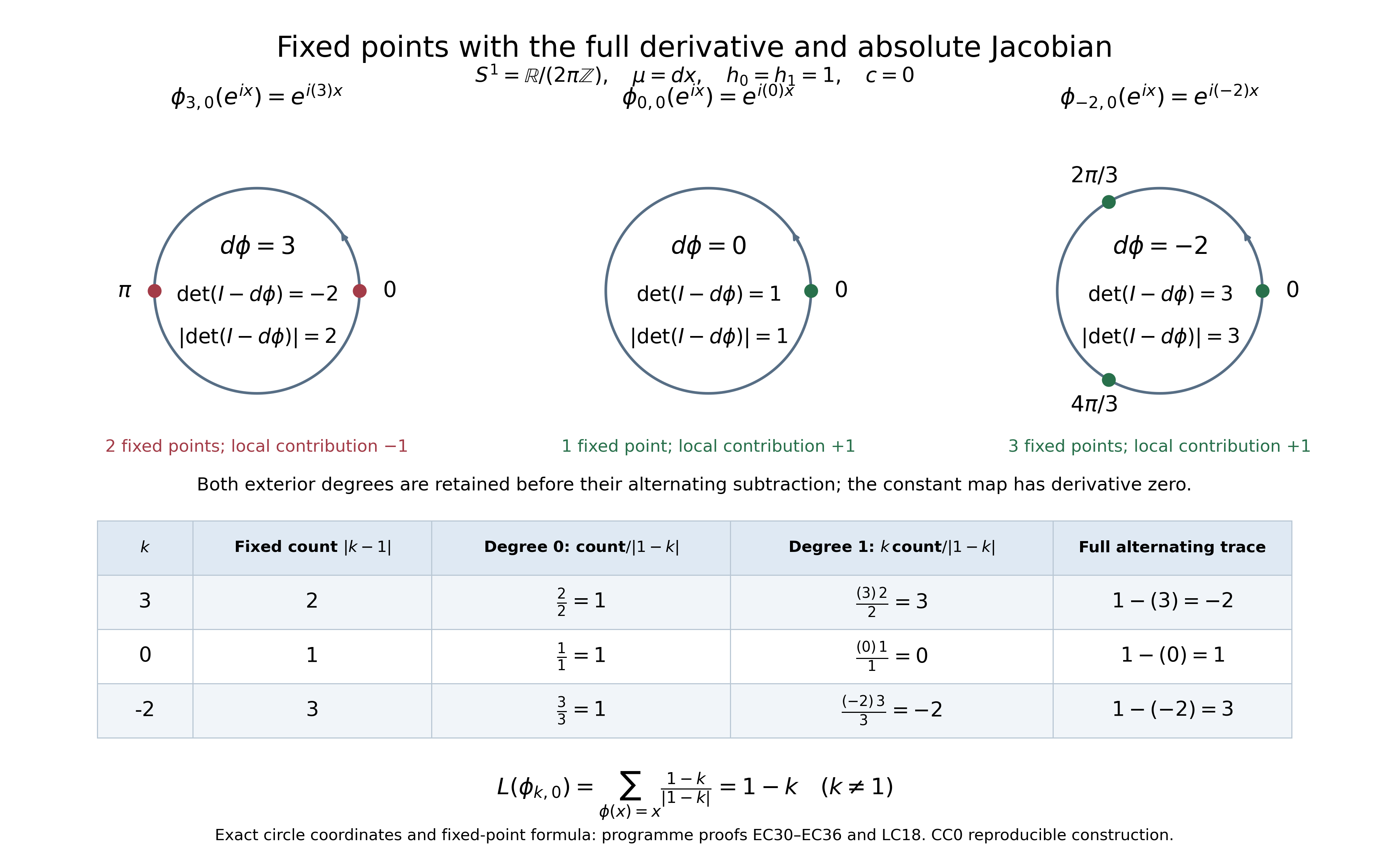
The figure uses the original circle angle modulo , density dx, unit displayed bundle frames and zero phase c. The marked angles are the exact fixed points of , not numerical zero estimates. The full derivative, signed determinant, absolute determinant and both exterior-degree contributions remain visible. The sampled curve depicts only the smooth unit-circle embedding. Its reproducible source is elliptic-complex-fixed-point-signs.py, and the complete proof is (EC30)–(EC36) and (LC18).
14. The exact circle metric choice and its full weight defect
The unit Fourier-frame computation in (EC37)–(EC38) uses the Hermitian metrics for which the displayed frames 1 and dx are unit. A density alone does not force these bundle metrics. Keep the original circle, density dx, differential ∂_x and half-density factor dx^(1/2), but now give those frames arbitrary positive smooth squared norms h_0(x),h_1(x). The full integration-by-parts identity gives Its precise difference from the displayed unit-metric adjoint is ; both coefficients are retained. Thus a nonunit metric changes the original adjoint and both full Laplacians, rather than being absorbed into the density. Positivity on the compact circle gives all actual weighted L² bounds.
The energy kernels are K_0=ℂ·1 and K_1=ℂ·h_1^(−1), and the complete projections are Each formula follows by retaining the original weighted inner product with its actual kernel generator and dividing by that generator’s full squared norm. Put ; its ordinary integral is exactly zero. The actual degree-lowering primitive is It is periodic because the full integral of v vanishes, and has zero h_0-weighted mean. Differentiation gives D_0G_0=I−H_1. For u=D_0f, its degree-one harmonic part is zero by the periodic fundamental theorem; (LC21) gives G_0D_0f=f−H_0f. This is the original G_0 from (EC12): both solve the same derivative equation with the same harmonic annihilator, and their difference is a constant with zero weighted mean. For a mean-zero periodic distribution v define its actual Fourier primitive . Its coefficients retain polynomial growth, hence define a distribution by the complete test expansion in (LC8). It maps H^s into H^(s+1): the full multiplier bound is for every n≠0. The extension of (LC21) is exactly . On smooth inputs the base-point constant in the integral from zero cancels in the weighted mean, proving agreement with (LC21). Both weighted projections are smoothing and have their full bounded distribution-smooth pairings, so this proves every stated Sobolev and distributional extension directly. For h_0=h_1=1 every formula returns the exact original Fourier operators, including 1/(in), n^(−2), the complete zeroth projection and every 2π factor. The two harmonic spaces and Euler index stay unchanged through the explicit comparison (LC13).
All strengthenings above have complete proofs for their written objects. The source-reading ledger distinguishes exact earlier programme proof reuse from new content reading and unread indexed literature.