Nonelliptic Fredholm operators on their exact adapted spaces
Written and dedicated to the public domain by Codex, September 2026 (CC0).
An operator can fail ellipticity at its largest differential order and still become Fredholm when its domain records the directions in which the full operator actually grows. This lesson proves that phenomenon for an infinite family. We keep the original Fourier multipliers, both anisotropic growth orders, every Sobolev exponent, and the complete domain and range. We also prove that the usual Sobolev realization at the largest order has dense, proper, nonclosed range.
Read Two-parameter Sobolev weights and conjugated operators for weighted Fourier norms, Finite defects under perturbation for the closed-range Fredholm criteria, and When finite defects force one-sided ellipticity for the distinction between standard and adapted domain-range pairs.
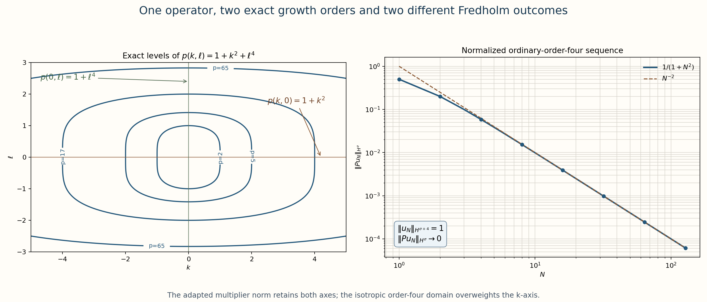
The left panel shows the exact level sets of . The right panel shows the normalized sequence that prevents the ordinary order-four realization from having closed range. The reproducible source is adapted_hypoelliptic_family.py.
1. A nonelliptic operator with two exact growth orders
On , use and . Define The order-four homogeneous principal symbol is , which vanishes at every nonzero covector . Thus is not elliptic of order four. The lower-order term is essential: it controls the direction missed by the principal symbol.
With , the complete multiplier satisfies Indeed, gives the first inequality, and expanding the square gives the second. Along , the multiplier has order two. Along , it has order four. A single isotropic order cannot describe both axes sharply.
2. The exact adapted domain
For , give its Fourier norm Define the domain determined by the full operator: Multiplication of Fourier coordinates by identifies this space isometrically with , so it is complete. Equation (AH2) gives both continuous inclusions Both inclusions are strict for every . The two complete axis sequences after (AH14) prove this, including every original weight.
For , define the Fourier coefficients The denominator is positive at every lattice point. Direct substitution gives the two exact norm identities The Fourier coefficients also show that and . Therefore
3. Why the ordinary order-four pair is not Fredholm
The map is bounded and injective. Let , where is chosen so that . Then If an injective bounded operator has closed range, its inverse on that range is bounded. That would give , contradicting (AH8). The range is dense because every trigonometric polynomial has a finite Fourier preimage. Section 6 below gives an element of outside the range, so the range is also proper.
4. Hypoellipticity from the same full multiplier
If is smooth, its Fourier coefficients decrease faster than every power of . Division by preserves that decrease, so is smooth. The reverse implication follows because a differential operator maps smooth functions to smooth functions. Hence This proves global regularity and supplies the adapted Fredholm scale. Local hypoellipticity requires a further argument, because the Fourier coefficients in (AH9) describe the whole torus. The local kernel proof after (AH21) supplies that argument for this operator and every member of the family below.
5. Every even-power anisotropic member
Fix integers and retain Its order- principal symbol is , so it is nonelliptic along the nonzero covectors .
For nonnegative , . Together with , this gives Because is an integer and , . Each term in is therefore bounded by , so
For , define The same Fourier-coordinate isometry proves completeness. The two full bounds give Both inclusions are strict. Fix any . Define two distributions by their only nonzero Fourier coefficients: These coefficients have at most polynomial growth, so both are distributions on the original torus. For , the full norms give The first estimate uses . For , retaining the different multiplier on its axis gives Here and for every . Since , both divergent exponents are at least . Thus and prove each strict inclusion in (AH14) separately, for every ; proves the same claim in (AH4).
Since , division is defined everywhere and Thus
6. Dense, proper, nonclosed ordinary range
On the ordinary pair , put Then , while The range is therefore not closed.
To prove that it is proper, define by Then . Its unique Fourier preimage would satisfy The inequality uses and . Since , the exponent is at least . Trigonometric polynomials still lie in the range, so the range is dense and proper.
The same rapid-decay argument proves the global equivalence:
Local hypoellipticity, with the full inverse kernel. For every open and every distribution , we prove Keep the full continuous multiplier , put , and let . For a multiindex , repeated differentiation of the actual reciprocal gives the finite ordered-partition formula The inner sum is over ordered nonzero multiindices. It follows by expanding to order using the finite Taylor expansion of in the reciprocal series: its -th term has sign , denominator , and ordered product of increments. The coefficient of , multiplied by , is exactly (AH26). Thus both factorials and every reciprocal factor have been retained.
For , ; for , . All mixed derivatives and derivatives beyond these two degrees are zero. Since and , each nonzero summand in (AH26) has the bound The same estimate for follows directly from . The continuous version of (AH11), , justifies the second inequality for every real . It uses , which does not require integer frequencies.
Let multiply each Fourier coefficient by . It acts on distributions and on smooth functions because . Coefficientwise multiplication proves on distributions. With ordinary Lebesgue measure on the torus, its convolution kernel is the distribution We now prove that this exact kernel is smooth away from modulo , rather than assuming that property. Define . The fundamental theorem of calculus, repeated times, gives There is the identical formula for with and the shift in . All signs and the whole shifted reciprocal are present. For a shift of size at most , the inequality shows that (AH27) gives For each nonnegative integer , choose so that . The Fourier series with either of these difference coefficients, and every spatial derivative of total order at most , then converge absolutely and uniformly. Indeed, grouping the lattice into dyadic annuli bounds the sum of , , by a constant times . The exact Fourier shift identities are At every point outside the torus origin, at least one of is nonzero. Divide the corresponding identity by its full smooth factor on a neighborhood of that point. The right side is . Since is arbitrary, is off the origin.
Suppose now that is smooth on . Fix an open with compact closure in , and choose equal to one on a neighborhood of . The exact distributional inverse gives The first summand is globally smooth: is globally smooth, its Fourier coefficients decrease rapidly, and multiplication by preserves that decrease. In the second summand, the support of has positive distance from . Choose a smooth cutoff in the integration variable equal to one on this support and supported away from . For , the second summand is the pairing of that distribution with the cutoff times . This is a smooth test function of , and all its -derivatives are smooth and uniformly bounded on compact subsets of , by the off-origin result above. Pairing with a distribution of finite order therefore permits every -derivative. The pairing equals : approximate by convolution with smooth approximate identities of shrinking support; the separated kernel pairings converge with all derivatives on compact subsets of , while Fourier multiplication by converges distributionally to the exact second summand. It follows that both summands in (AH32) are smooth on . Such sets cover . The reverse implication in (AH25) follows from locality of the differential operator. This proves local hypoellipticity for every , including the original , without changing any adapted norm or multiplier.
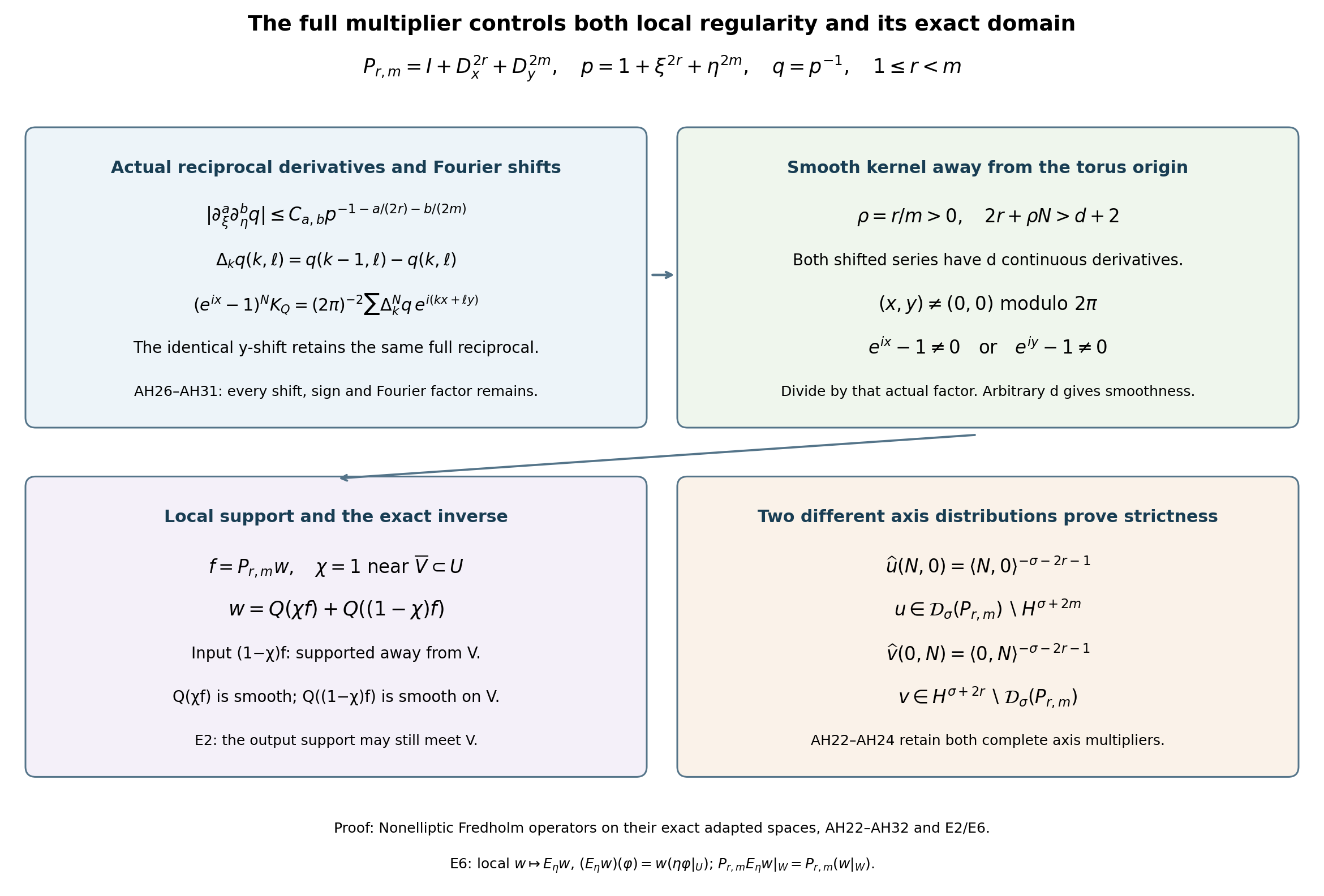
The diagram records the exact reciprocal, its two Fourier difference identities, the separated support in (AH32), and the two actual distributions proving strictness in (AH22)–(AH24). The proofs are (AH25)–(AH32) and (AH22)–(AH24). The reproducible source is adapted-local-kernel.py.
7. Worked member: orders four and six
Take and . Then On the normalized -axis sequence, the ordinary order-six output is The same operator is therefore an isometric bijection on its adapted domain and non-Fredholm on the ordinary order-six pair.
8. Exercises with solutions
Exercise 1. For , state the two Sobolev spaces that bound its adapted domain and compute the decay power of the normalized ordinary order-six sequence.
Solution. Equations (AH11)–(AH14) give Along the -axis,
Exercise 2. Compare the adapted norm with the usual graph norm .
Solution. Since , Consequently The adapted norm is exactly the output norm and is equivalent to the full graph norm with the displayed constants.
References
The theorem proved here is the explicit -family above; it does not state that every operator in those broader classes has been reduced to this Fourier model.
Editorial supplement: the original torus inverse, exact domains and sharp consequences
Editorial proof completed in October 2026; CC0.
This supplement supplies the Fourier and distribution receivers of (AH3), (AH13) and (AH25)–(AH32), and proves further consequences for the same operators. Equations (AH1)–(AH32), their original order, both worked solutions and (AF1)–(AF2) above remain unchanged. Throughout, are integers, , the torus has period in each coordinate, and . Every norm below is the original Fourier norm. The weighted Euclidean norms in the earlier Sobolev lesson, (MSB3)–(MSB5) explain the preceding reading link; the torus statement and its measure factor are proved here. No general nonelliptic Fredholm theorem is needed. The scalar and finite-coordinate derivative, Taylor and real-power rules are proved in the metric foundation, Sections 13.1–13.8. The integrations and linear substitutions below use the Banach foundation, (LP1)–(LP5), restricted to the original torus coordinate box when the domain is compact. They supply absolutely integrable Fubini and the complete translation and scaling Jacobians; the only nonnegative infinite sums below are increasing limits of finite sums. The torus boundary faces have Lebesgue measure zero by that foundation’s full box-volume argument.
E1. The torus Fourier and distribution maps
Put , , and . Use complex-linear distribution pairing and ordinary Lebesgue measure, with the exact convention The period, derivatives and complete orthogonality integrals of these characters are proved in the metric foundation, (OC33)–(OC37), including the original zero-mode integral . In particular its addition laws give , the precise factor used in the finite geometric estimate below. Boundary integration by parts has no boundary term for periodic smooth functions. For every integer , . Thus smooth functions have rapidly decreasing coefficients. Conversely, if for every the coefficients satisfy , the series , and each differentiated series, converge absolutely and uniformly. To verify summability, a dyadic shell contains at most points. Consequently for . Repeated integration of the uniformly convergent derivative series proves that their sum is smooth and has precisely the specified coefficients.
Here is also the required uniqueness, rather than an assumption that the characters are complete. For , define the finite trigonometric polynomial The second identity follows by counting the ordered pairs of indices whose difference is . Thus and . Away from zero modulo , the finite geometric sum gives . Therefore the ordinary Lebesgue convolution kernel has mass one and its mass outside any fixed neighborhood of the torus origin tends to zero. For a continuous function, split into that neighborhood and its complement. Uniform continuity bounds the first part by its modulus of continuity; the second part is bounded by times the mass just estimated. This proves uniform convergence. For smooth functions the same proof applied to each derivative proves convergence in every smooth seminorm, since differentiation commutes with convolution with this finite polynomial. A continuous function with all Fourier coefficients zero consequently vanishes. Applying this to the difference of a smooth function and its absolutely convergent Fourier series proves its reconstruction, including all derivatives.
On the compact torus a distribution means a continuous linear functional on , whose defining seminorms are . Continuity at zero gives one integer and a constant such that Indeed, a finite intersection of seminorm balls lies in the inverse image of the unit disk; replace their orders by their maximum and scale the test function. Testing exponentials proves polynomial growth of . Conversely, if , define Choose an integer with . The integration-by-parts bound above proves absolute convergence and bounds (AE4) by a constant times the supremum norms of derivatives of through order . Thus it is a distribution, and direct testing in (AE1) gives . Finally, the smooth reconstruction of converges in every seminorm, so every distribution applied to that reconstruction equals (AE4) with its own coefficients. This proves distributional uniqueness and all the maps just used.
In particular, if , both and have polynomial growth: and . Equation (AE4) proves that they really define distributions. The two coordinate maps are therefore onto isometries, with the displayed inverse coefficient maps. Enumerate the origin first, then each finite square shell , , in lexicographic order. This is an explicit bijection , and pullback of coordinates preserves every nonnegative squared sum. Completeness of , proved in the Banach foundation, Section 11, proves both completeness assertions; coordinate truncations prove density of finite Fourier polynomials in both spaces. The same bounds show that norm convergence there implies distributional convergence. Orthogonality of the characters, integrated with ordinary Lebesgue measure, gives for every finite polynomial . An -Cauchy polynomial sequence has an ordinary limit by the Banach foundation, Section 15.3. Testing against a smooth function and Cauchy–Schwarz identifies that limit with the distribution supplied by (AE4). Passing the finite norm identity to the limit retains precisely the factor .
Since differentiation multiplies the coefficients by or , (AE5) proves the actual maps, both inverse products and every norm identity in (AH5)–(AH7) and (AH15)–(AH16). Their kernels and cokernels are zero and their ranges are the entire Banach target, so the index is zero in the definition of the Fredholm lesson, (F1). The power inequality preceding (AH11) follows from convexity of , or directly its nonnegative second derivative for and equality for . Its continuous version uses ; the lattice version of (AH12) uses . Thus their stated constants and all the inclusions are valid. Equations (AH22)–(AH24), now genuine distributions by (AE4), establish their stated strictness. The same construction proves the existence of (AH19), whose squared norm is . Its preimage is excluded by the complete calculation (AH20), while polynomial density proves density of the ordinary range. A dense proper linear subspace is not closed. Alternatively the closed-range inverse assertion used in (AH8) follows by applying the proved bounded inverse theorem, (B8)–(B9) to the injective map onto its closed Banach range. Its lower bound contradicts the exact sequence (AH18). This supplies both arguments at every real . Rapid decay and multiplication by the original polynomial prove (AH9) and (AH21) in both directions.
E2. The full local kernel and the separated distribution pairing
The finite expansion used in (AH26) can be justified without any formal infinite series. At a fixed , put . For small , , and the finite geometric identity with remainder gives Take . Since , every derivative of the remainder through order at zero is zero, by the finite Leibniz rule. Expanding each increment by its actual polynomial Taylor formula and differentiating the coefficient of proves exactly the ordered sum (AH26), with both factors retained. A nonzero derivative factor is a pure - or pure -derivative, and its exact factorial gives respectively a bound or . Multiplying the factors in their given order and the actual gives the first estimate (AH27). Raising the continuous lower bound (AH11) to the positive power gives its second estimate with exponent . Since , the third estimate follows with every exponent as written. The zero multiindex is covered by the direct reciprocal.
Polynomial-growth and rapid-decay sequences in E1 show that multiplication by defines on distributions and on smooth functions; the latter map is continuous in the smooth topology. Indeed the integration-by-parts estimate and the summability bound in E1 bound each output derivative seminorm by finitely many input derivative seminorms. The even identity gives under the complex-linear convention. Consequently distributional convergence of implies that of . Their exact coefficient products are one for and .
The ordinary convolution of smooth functions has Fourier coefficients : substitute in its defining integral. The coefficients of (AH28) are , so its convolution with a smooth function has exactly coefficients . Equivalently, distributional convolution with a smooth function is the pairing with its translated smooth test function; (AE4) gives the same coefficients. This proves the kernel formula with its ordinary measure.
For completeness, the Fourier coefficient of at is , so iteration of the actual difference proves both identities (AH31) as distributions. The repeated fundamental theorem of calculus proves (AH29), including and the entire shift. For , the triangle inequality in applied to gives . This proves (AH30). For any requested derivative order , choose an integer with . The explicit lattice summability bound in E1 makes both right sides of (AH31) . Division by the specified nonzero smooth factor works on its own neighborhood. These distributional representatives agree on overlaps because distributional reconstruction is unique. Taking arbitrary therefore proves that the original is smooth off the torus origin, with no choice of an alternative inverse kernel.
We now verify the cutoff and limiting operations in (AH32). The smooth cutoffs used here are supplied by the explicit compact bump construction in the metric foundation, Section 13.10, (OC38)–(OC41). For a compact set contained in an open set on the torus, cover it by finitely many coordinate balls whose closures lie in that open set. On each ball the Euclidean bump construction gives , equal to one on a smaller ball, and supported inside the original ball; extension by zero is smooth. The finite expression is the desired cutoff, equal to one on a neighborhood of the compact set. This proves the stated torus cutoff receiver, including the case of the whole torus.
The distance here is the original flat quotient distance . The minimum is attained: for representatives in , the zero shift already gives a fixed finite upper bound, so all larger shifts can be excluded and only finitely many remain. The triangle inequality follows by adding the minimizing shifts, and distance varies continuously by that inequality. The torus is compact, being the continuous image of the original compact square. Thus two disjoint compact sets have a positive minimum distance: distance attains a minimum on their compact product, and a zero minimum would give a common point. This supplies the exact support separation used next. Every point of an open has a small metric ball with compact closure in , by taking half the radius of a ball contained in ; such cover . For empty , both local assertions are vacuous.
Set with and the original near . Its support is a compact set disjoint from a neighborhood of , hence has positive distance from if it is nonempty. Choose by the preceding construction a cutoff equal to one on a neighborhood of and with support a positive distance from . If , the second term is zero and there is nothing to pair. Otherwise, for , the function is well defined. The test function in (AE7) is globally smooth in , since its cutoff is zero near the possible singularity . All its mixed derivatives are bounded when ranges over a compact subset of . Taylor’s formula with uniform derivative remainders in the seminorm of (AE3) proves that difference quotients of (AE7) converge to the pairing with the corresponding -derivative. Repeating this proves .
To identify this particular pairing with the actual , choose a nonnegative , supported in the unit ball, with . The bump just described divided by its positive integral gives such a function, retaining that integral in the normalization. For , periodize its original scaling: The sums are locally finite. Substitution , with Jacobian , proves mass one on the original torus and the displayed coefficient. The convolution is smooth, since it is the distribution pairing with a jointly smooth kernel. Its support is contained in the torus -neighborhood of . Testing convolution against a smooth function amounts to convolving that test function with the reflected ; the mean-value bound for every derivative proves convergence to that test function in . By (AE3), distributionally. Its Fourier multiplier is the full integral on the right of (AE8), since the convolution coefficient cancels the explicitly displayed ; the integral is bounded by one and tends to one.
For sufficiently small , on . Convolution of with the smooth , already identified by its exact coefficients, can then be restricted to the region away from the singularity for . It equals there, with ordinary measure and no extra factor. This can also be checked by testing in with a compactly supported smooth function in : the distributional kernel is paired only against tests supported away from its origin and therefore equals its established smooth representative there. As , all derivatives of these pairings converge uniformly on compact subsets of to those of (AE7). Indeed, reflected convolution converges uniformly in every seminorm on the compact family of joint derivatives of , and (AE3) bounds the errors. On the other hand distributionally by the proved transpose formula for . Thus (AE7) is exactly the restriction of to . The first term in (AH32) is globally smooth, since extends smoothly by zero and has rapidly decreasing coefficients. This proves the forward direction of (AH25) on every such , hence on . The reverse direction follows from the local derivatives defining , so all of (AH25) is proved.
An editorial clarification to the existing diagram is needed: the sentence “Second term: its support stays away from V” in refers to the input distribution . The support of its output need not stay away from . The exact assertion proved by (AE7)–(AE8) is that this output is smooth on . This identifies the support ambiguity while retaining the original diagram and its reproducible source. There is an explicit counterexample to interpreting it as a support assertion about the output. Choose a small coordinate rectangle and an open with closure inside it, containing the chart origin. Put . The factorial bound makes this series and every derivative uniformly convergent on compact intervals; shifting its index proves . Since , choose the rectangle small enough that there, and a smooth cutoff supported in that rectangle and equal to one on a neighborhood of . The globally smooth function , extended by zero, satisfies where , since and its -derivative there is zero. Choose the original-type near supported within that neighborhood. For , one has , hence and , which is nonzero on . Its input support is separated from , and its output is smooth and nonzero there. More generally (AE7) is the exact linear map from distributions supported in to smooth functions on . For a distribution satisfying (AE3) with order , its derivative of order is bounded on any compact by . Thus the actual support defect gives a proved smooth receiving map rather than a false support-preserving assertion. The continuous level curves in the first existing figure are the continuous -section of the same full polynomial; the actual Fourier indices of the operator remain the lattice .
E3. Exact derivative domains and the unbounded realization
There is an additional exact domain description, with its original norm retained: The arrows in this equality are identity maps on distributions. To prove both directions and their norm bounds, set . The full expansion and finite Cauchy–Schwarz inequality give The inequalities hold first term by term, then after summing nonnegative terms, including infinite sums. They prove (AE9), its bounded inverse identity maps and the presence of every original cross-term. The graph norm comparison in Exercise 2 follows independently from , with its exact constants one and two.
Regard the same differential operator as an unbounded operator on the original . Its maximal domain is exactly (AH13): coefficientwise this condition is , and ensures the required input membership. It is densely defined, closed, positive and selfadjoint. These assertions can all be verified on the exact orthonormal basis Density follows from E1. If and in , each coefficient converges, giving . The maximal-domain condition then proves closedness and . For in this domain, , with convergence by Cauchy–Schwarz. The same coefficient calculation proves symmetry. If a vector is in the adjoint domain, testing against every basis vector in (AE11) forces the coefficients of its adjoint image to be times those of . Square summability of that image is exactly the maximal-domain condition. Conversely that condition makes the symmetry identity valid for every input by Cauchy–Schwarz, and hence puts in the adjoint domain. This proves selfadjointness, without an imported unbounded spectral theorem. Finite Fourier truncations converge in both input and output norms, so these polynomials form a graph core for this actual realization.
Its inverse on is the same full . Its norm is one, attained at the origin frequency; it is positive and compact. For compactness, truncate to . The operator-norm error is , by (AH11). Finite-rank maps are compact, and an operator-norm limit of them is compact: for a prescribed error choose a truncation with smaller norm error and a finite net of its bounded image; this gives a finite net of the full image. For any sequence in its closure, successive finite nets of radii allow nested subsequences contained in a single net ball at each stage; the diagonal subsequence is Cauchy. Completeness gives its limit in that closed set. The metric compactness equivalence proved in the Banach foundation, Section 10 then proves compactness.
The spectrum of the unbounded realization is exactly the set of numbers , with each original lattice multiplicity. Every such number has its basis eigenvectors. If is not in that set, the set has only finitely many elements in each bounded interval, because bounds both and . It follows that and . The coefficient map is therefore bounded from into the exact domain (AH13), and verifies both inverse products for . It is in particular a bounded inverse into ; this proves the claimed spectrum with the original domains.
E4. Sharp isotropic gain, compact embeddings and every bounded ordinary pair
For every real , the exact coefficient map for the prospective , initially on finite Fourier polynomials, has the supremum of its output-to-input norm ratios The upper estimate follows by summing squares; testing the original basis (AE11) gives equality, including an infinite supremum when no bounded extension exists. If the supremum is finite, completeness and core density give its unique bounded extension; distributional convergence identifies that extension with the original . For , (AH11) bounds this ratio by . For , the ratio on tends to infinity. Consequently For the compact direction the same finite truncations have norm error at most . At , the images of the orthonormal inputs are orthogonal in the output space and their norms tend to one, so they have no convergent subsequence. For the operator is not bounded and hence is not compact. Composing with the exact isometry proves the identical sharp boundedness and compactness conditions for the inclusion . These are actual identity inclusions, not a replacement for the adapted norm. In fact for the inclusion fails even as a whole-space set inclusion. Put , and give only the coefficients , . This is a distribution in , with squared norm . Its exact preimage has squared norm at least . The bound uses and the positive numerator exponent . A one-dimensional dyadic shell contains at least integers and bounds each power by a fixed positive multiple of ; its sums therefore diverge when . This also proves the endpoint domain claim as an actual distributional inclusion statement.
The original constants in (AH11)–(AH12) also admit an exact additional comparison on this lattice. Since is an integer, , so the same power inequality gives . The multinomial expansion of contains the three nonnegative terms , and , with all its other nonnegative summands retained. Since , it gives , including every original summand in . The corresponding exact operator norms are The first upper bound just proved is attained at , where and . The second is attained at the original origin frequency , with upper ratio . Thus the endpoint domain inclusion in E4 has norm , through the exact isometry (AH16). These sharpenings do not change the continuous reciprocal estimate, which still uses the original full bound in (AH27); the integer-frequency inequality is not assumed for noninteger .
Similarly, the ordinary map is bounded exactly when . For these , (AH12) bounds its coefficient ratio by . For , its ratio at tends to infinity. Every bounded such ordinary map is injective with dense, proper, nonclosed range. Injectivity uses , and density follows from polynomial preimages. The same fixed target (AH19) belongs to , while its unique distributional preimage has full ordinary squared norm Here , , and . Thus the original (AH20) is the endpoint case . The corresponding normalized ordinary input is , and its output norm is . Both the proper-range proof and the lower-bound contradiction therefore propagate to every bounded ordinary pair, with all original multipliers.
For (AF1)–(AF2), take : the strict domain bounds are exactly , and the displayed ratio is asymptotic to . For Exercise 1, gives the original strict bounds and its exact ratio , whose quotient by tends to one. The general results also show compact domain inclusion into every with , but not into its stated upper endpoint .
E5. Exact lattice multiplicities and the sharp inverse summability threshold
Let count the eigenvalues of the original unbounded realization not exceeding , with multiplicities. It is zero for . For , retain , set , , , , and . Every lattice point satisfies . Separating the four open quadrants, both axes and the origin gives the exact finite formula The sum is empty if its upper endpoint is zero. Its summands are nonnegative, including a zero at any exact horizontal intercept; axes are counted by the two additional terms and the origin by the final one. In particular , not zero.
For , the continuous function decreases from to zero on . Extend it by zero after . On each unit interval its integral lies between its endpoint values. Summing these finite inequalities gives , where ; the last partial interval is included by the zero extension. Subtracting the floors loses at most . The substitution , including Jacobian , yields , with the exact positive constant For the upper bound in (AE16), use the upper bound on the floor sum in (AE15) and . For the lower bound, use and . The resulting lower error is at least ; the upper error is at most . This proves (AE16) also at directly. Since , its full error divided by tends to zero, and . Thus , with the retained shift in the exact formula and bound.
All singular values of the compact positive inverse on the original are the numbers , listed with every lattice multiplicity. To verify this without invoking an unbounded spectral theorem, the explicit basis (AE11) diagonalizes , and its positive square root is the diagonal map with those positive numbers. For uniqueness, if a bounded positive satisfies , then . Positivity gives , so its kernel is zero. Hence for each , and density makes . Its finite-dimensional eigenspaces are precisely their lattice spans, and the basis is complete by E1. Its only additional spectral point can be zero, since the numbers tend to zero; inversion of any other diagonal difference with positive distance proves this as in E3. For , membership in the Schatten class means summability of the -th powers of these singular values (also when ). For this operator the exact criterion is Here is the endpoint proof. From (AE16), for all , after increasing a finite constant. In the shell , . The resulting geometric series converges if , with the origin contribution retained separately. Conversely, the proved asymptotic gives For all sufficiently large , each shell therefore contains at least eigenvalues, for some fixed . Every one has , so its sum is at least . The disjoint shell sums diverge for , including the equality endpoint. This proves (AE17) at its full stated generality for every .
In particular , so every original inverse is trace class and has exact trace and trace norm This agrees with the original trace-ideal definition in the trace lesson, (T5). Indeed, for finite paired orthonormal systems , expand in (AE11). The triangle inequality and finite Cauchy–Schwarz give . The last bounds follow from the norm of each orthogonal finite projection of ; its squared norm is at most one by the Pythagorean identity. Taking both systems from the actual basis gives the reverse inequality after increasing finite subsets. Thus the defining norm (T5) equals the full sum. For any complete orthonormal basis , nonnegative summation gives : the inner sum is one because finite orthogonal projections converge to the vector in a complete basis. This proves the trace assertion and its basis independence directly for this actual operator. The finite positive diagonal truncations also converge in that trace norm, since their full tail sums tend to zero.
This summability also strengthens the kernel statement at its actual origin. The full series (AH28) now converges absolutely and uniformly on the entire torus: its uniform tail is at most times the corresponding positive tail in (AE19). Its continuous sum has the original distributional coefficients by (AE1), so E1 identifies it with the same , including its off-origin representative in E2. At the origin all summands are positive, giving the exact identities The upper norm bound is the triangle inequality for the full uniform series, and its equality follows from that origin value. This does not assert nonnegativity of at other points. It also does not assert smoothness at the origin: coefficientwise the exact product is , since both sides have Fourier coefficients . The delta distribution cannot be represented by a continuous function. In fact, choose smooth cutoffs , equal to one at the origin and supported in a coordinate ball of radius . Their integrals are bounded by the full area for small and tend to zero. Pairing any bounded continuous function with them tends to zero, whereas . If were globally , its original differential image would be continuous, a contradiction. Thus this same kernel is globally continuous, smooth away from its actual origin, and not globally . Every Fourier factor and the original differential order are present in this comparison.
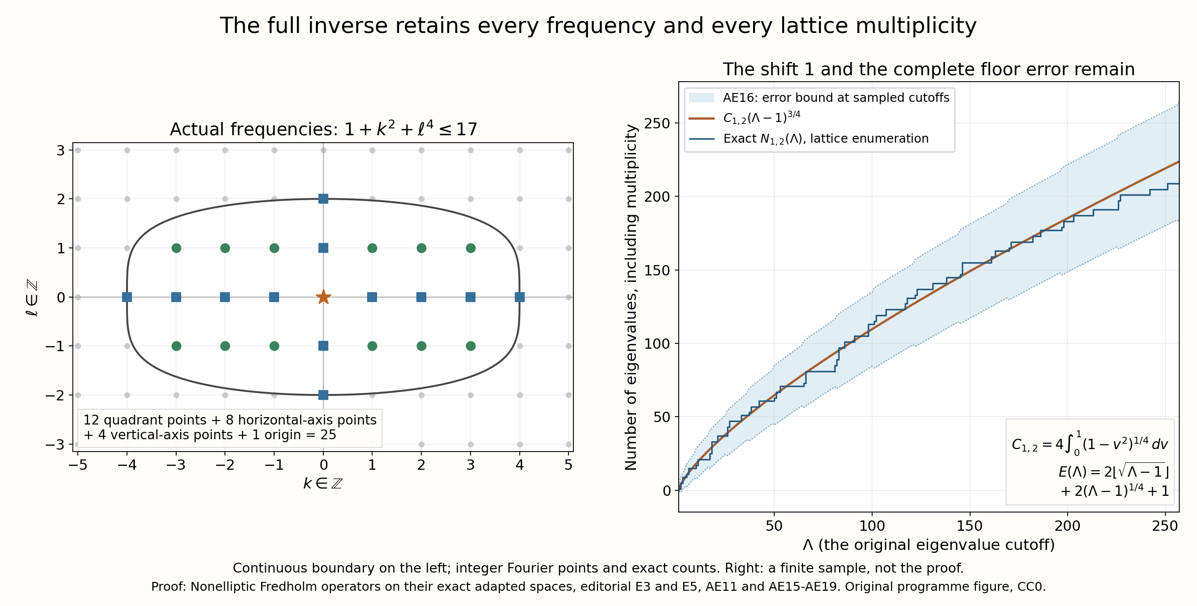
The left panel is the actual integer-frequency spectrum below for the original operator; its boundary is the continuous section , not an additional frequency set. The origin and both axes are counted separately in (AE15). The right panel compares the exact staircase with and the proved full error bound in (AE16), including the shift, the floor, and the final one. The graph is a finite numerical sample of that proved inequality, whose proof is E5. The reproducible source is adapted-exact-spectrum-264.py.
E6. Distributions defined only on the open set
The theorem (AH25) was stated for a distribution on the entire torus. Its conclusion also holds for a distribution defined only on the given open set. We prove the precise extension and restriction maps, using the same operator with the original integers . The derivatives and the measure are the original period- torus ones.
Write . Its distributions are linear functionals continuous on each space of tests supported in a fixed compact , with seminorms . This is the distribution convention already used in E1–E2. Restriction to a smaller open set means evaluation on the zero extension of its compactly supported tests; that zero extension is smooth because its support is contained in the smaller open set.
Fix a point . Choose so that the closed coordinate ball of radius about is contained in a coordinate chart inside . Let be the ball of radius . There is a smooth cutoff supported in that closed larger ball and equal to one on the ball of radius . Here is an explicit construction that also fixes its support. Put for and for . Each derivative on the positive half-line is an exponential times a polynomial in , which tends to zero as : indeed implies . Thus is smooth. In the chosen chart set and , extending it by zero outside the chart. The denominator is positive everywhere in the chart: its two summands could both vanish only if and . This cutoff is one for , zero for , and its zero extension is smooth. In particular it is one on a neighbourhood of . Let .
For define an actual distribution on the whole torus by For the fixed compact , continuity of supplies a finite order and with for . The full product rule gives Every summand and cutoff derivative is retained. This is a finite continuous seminorm bound on torus tests and proves that (AE21) has its stated codomain. The map is linear. With the topology of convergence on every fixed test in each distribution space it is continuous, since evaluation of its image on is exactly evaluation of its input on the fixed test .
For any we have . The formal transpose of this particular operator is itself: each derivative has even order, and its coefficient remains respectively . Moreover , so . Consequently the exact restriction identities, with all domains shown, are To verify the second line on a test rather than suppress a cutoff contribution, its left-hand side is . The right-hand side has exactly that value by the definition of the local distributional derivative. The equality is after restriction to , where the cutoff is identically one; no global commutation of with multiplication by is asserted.
Suppose now that is represented by a smooth function on . By (AE23), is smooth on . Apply the already proved theorem (AH25) to the global distribution and the open set . It gives a smooth representative there. The first line of (AE23) identifies that representative with . The balls obtained for all points cover , so is smooth on .
For completeness, the local smooth representatives agree on overlaps. If their difference had a nonzero value at a point, multiplication by a fixed complex unit would make its real part positive on a smaller ball. A nonnegative, nonzero smooth test supported in that ball would then give a nonzero distributional value, contradicting equality of the restrictions. They therefore patch to a unique smooth function. It represents the original distribution on every test: a compact test support has a finite cover by the balls above, and smaller cutoff balls give smooth functions supported in those balls with near that support. Decompose the test there as , with zero extensions where the denominator is not needed. Each summand has compact support in its ball and has the corresponding representative. Their sum gives the original pairing with the function using .
Conversely a smooth has smooth by the displayed finite differential formula. Thus for every open and every , smoothness of on is equivalent to smoothness of there. The empty set has only its zero distribution, so is included. The argument also applies when is the entire torus; no extension outside the torus is used. This strengthens the domain of (AH25) and leaves the distinct adapted Fredholm and ordinary Sobolev assertions unchanged.
The local-kernel figure now labels the input , whose support is separated from , and its smooth output , whose support may meet . The exact receiving map and counterexample proving this distinction are in E2. Its footer also displays (AE21) and the restricted operator identity (AE23), which allow the same local argument for distributions initially defined only on . These are original programme proofs, with the same CC0 dedication and without an external proof citation.