Traces that survive passage to cohomology
An index can be recovered from a difference of traces even when neither operator being compared has a meaningful trace. A complex introduces a second cancellation: contributions from the boundaries occur in adjacent degrees with opposite signs. This lesson proves both mechanisms, including the case of closed unbounded differentials with nonclosed ranges.
All Hilbert spaces are complex and may be nonseparable or zero-dimensional. Inner products are linear in the first variable. An operator without a domain qualification is bounded and everywhere defined. A sum of nonnegative numbers indexed by an arbitrary set means the supremum of its finite subsums. An absolutely summable complex family has a sum independent of ordering, defined by finite-subset limits. A finite nonnegative sum has at most countably many nonzero terms: for each positive integer , only finitely many terms can exceed .
Begin with a three-term complex
Before introducing operator ideals, one can see the cancellation in a complete finite-dimensional model. Use the coordinate Hilbert spaces , , , with respective bases , , and . For an arbitrary complex parameter , retain both matrices
For arbitrary , put
The first product and the product both send to and to zero. The products and both send to and the other basis vectors to zero. Thus these three maps define an endomorphism of the entire complex for every , including zero.
The finite-dimensional trace is the sum of diagonal entries. It is independent of the basis: for two composable rectangular matrices, summing every product entry gives ; apply this identity to a basis-change matrix and its actual inverse. In this model the full alternating trace is
For , the three cohomology spaces are respectively , , and : the boundary removes one direction from , and the boundary removes one direction from . Their induced maps are multiplication by . Their alternating trace is exactly (T52).
At , the first cohomology space is all of , the middle one is , and the last is still . Their induced traces are . The alternating sum again equals (T52). Two cohomology dimensions jump, and the added -contributions cancel in adjacent degrees.
This calculation sets the questions for the infinite-dimensional proof. A diagonal sum needs a basis-independent convergence estimate. A boundary range may fail to be closed, so its closure must be distinguished from the actual range. An unbounded differential needs its graph domain before an intertwining product can be used. Sections 1–5 construct those analytic tools; Section 6 proves the cancellation on reduced cohomology, Section 7 recovers the index from error powers, and Sections 8–9 handle parity and tensor products. The nonclosed-range and noncompact-error examples in Section 10 show why these are different questions.
1. Hilbert-space contracts and square-summable operators
The following Hilbert-space and operator facts are used with the stated domains and limits. The Banach and Fredholm tools appear in Banach estimates, quotient spaces and compact parameter arguments and Finite defects under perturbation.
Section 6 of Spectral measures with the original operator domain retained proves the Hilbert interfaces in full: (HF1)–(HF5) give projections, arbitrary orthonormal bases and bounded adjoints; (HF6)–(HF9) give the unique positive root with its actual moment domain; (HF10)–(HF17) prove , the polar isometry and every finite-band inverse; and (HF18)–(HF19) construct the Hilbert tensor completion. These proofs allow nonclosed ranges and arbitrary Hilbert dimension. The finite-dimensional compactness facts retain the exact Banach-foundation route.
- Hilbert-space geometry. Arbitrary Hilbert spaces have orthonormal bases; Parseval’s identity and orthogonal expansions hold as finite-subset limits; closed subspaces have orthogonal projections; bounded operators have bounded adjoints with , and . Finite-dimensional Hilbert spaces have the usual compactness and dimension properties.
- Positive square roots. Every bounded positive selfadjoint operator has a unique bounded positive square root. The root squares to the original operator and has the expected quadratic-form identity. No compactness or countable spectral basis is assumed.
- Closed-operator polar decomposition. If is closed and densely defined, is positive selfadjoint, has domain , and , where is a partial isometry from onto . For a positive selfadjoint , its spectral projections satisfy , commute with on , obey on , and converge strongly to the projection onto . On , is a bounded bijection with bounded inverse given by the spectral function .
- Hilbert tensor products. The algebraic tensor product with inner product has a Hilbert completion. Tensor products of orthonormal bases form an orthonormal basis of that completion. Basic scalar series and finite-product operations are understood. We verify the operator estimates and the Hilbert-Schmidt realization below.
- Measure facts (optional realization only). completeness, product integrals for elementary products under the primitive countable rectangle-cover product measure, and approximation of functions by simple functions supported on sets of finite measure. The abstract tensor and index proofs use no measure realization.
- Banach-space tools. Banach completeness, the bounded inverse theorem, and the uniform boundedness theorem for arbitrary pointwise bounded families. These two results and their assumptions are given in Section 1 of Finite defects under perturbation.
- Compactness facts. Compactness of finite-dimensional balls, metric sequential compactness, and the fact that a uniform limit in operator norm of compact operators is compact. For the last fact, finite -nets for the approximants’ unit-ball images give total boundedness of the limit image.
- Fredholm tools. Sections 2–5 of Finite defects under perturbation give the compactness characterization and norm stability of upper semi-Fredholm maps, Fredholm composition, and the two-parametrix criterion. This lesson uses the version in which no range complement is assumed in the upper semi-Fredholm case.
Let be an orthonormal basis of . For , set
The operator is Hilbert-Schmidt when this is finite; the class is denoted .
Theorem. Formula (T1) is independent of the basis. The adjoint has the same Hilbert-Schmidt norm. The class is complete in that norm, contains every finite-rank operator densely, and
for bounded maps of the indicated source and target spaces. Every Hilbert-Schmidt map is compact.
Proof. Choose an orthonormal basis of . Parseval, followed by the definition of a nonnegative double sum, gives
Both orders of summation equal the supremum over finite subsets of . For any finite subset of the product, its two coordinate projections are finite, so finite rectangles give the same supremum. Fixing either basis in (T3) proves independence of the other, and proves adjoint equality.
For a finite orthogonal expansion , Cauchy-Schwarz gives ; passing to the dense span proves the first estimate in (T2). The left ideal estimate follows directly from . Taking adjoints gives the right ideal estimate, and combining them proves (T2).
If has finite rank, then is finite-dimensional. Here equality follows because the finite-dimensional range of is closed and its orthogonal complement is ; finite rank of follows by writing in coordinates in its finite-dimensional range. A basis adapted to makes (T1) a finite sum. Conversely, if (T1) is finite, let project onto the span of a finite subset . Then
Thus finite-rank maps are dense. One can choose a sequence of finite sets giving errors below ; no countability of is being assumed. The operator norm estimate makes the same approximation converge in operator norm, so is compact by the compactness facts.
For completeness, a Hilbert-Schmidt Cauchy sequence is operator norm Cauchy and has a bounded operator limit . The existence of the operator norm limit follows by taking limits in the Banach target and passing linearity and the uniform norm bound to those limits. For each finite ,
Taking the supremum in proves both and . The mixed sum converges absolutely by Cauchy-Schwarz; polarization of the basis-independent squared norm makes it a basis-independent inner product. Together with completeness, this makes a Hilbert space.
Nonseparability causes no missing sums here. For a Hilbert-Schmidt , only countably many basis vectors have nonzero image, and the range is contained in the closed span of their images. It is the operator’s effective support that becomes separable.
2. The trace ideal from paired orthonormal systems
For , define
The same finite set labels the two systems; they need not be complete bases. The value may be infinite.
Theorem: factorization. The following conditions are equivalent:
- .
- For every pair of orthonormal systems with a common, possibly infinite index set, .
- For some Hilbert space , there are and such that .
When these hold,
where the last sum is over any orthonormal basis of . In particular, the infimum is attained by a factorization constructed below.
Proof. If , then for any paired systems,
Extend each orthonormal system to a basis to justify the last inequality. Finite sums and then suprema justify Cauchy-Schwarz for arbitrary indices. Thus 3 implies 1, and 1 implies 2.
Suppose 2. Put and . Indeed . The map is a well-defined isometry on , whose closure is . Extend it continuously to , and by zero on , obtaining a partial isometry with . This is a direct construction of the bounded polar factor, using only the positive square root contract.
Choose an orthonormal basis of . Then is orthonormal in , so condition 2 gives
Let . Its kernel is : , and . Therefore . A basis of contributes zeros, so (T8) and (T1) give . Since is isometric on , . Take
Then , and by adjoint equality. On the other hand, the finite parts of the paired systems in (T8) show . Inequality (T7) proves the reverse inequality and the infimum formula. The final sum in (T6) is independent of basis because it equals . This also covers , with zero factors.
The distinction between the existence of a Hilbert-Schmidt factorization and a statement about arbitrary specified factors is essential. A trace-class product does not force its two given factors to be Hilbert-Schmidt; the zero operator composed with the identity on an infinite-dimensional space is an immediate counterexample.
Define to be this class, and .
Theorem: norm and ideal properties. This is a Banach space. Finite-rank maps are dense, and for bounded , ,
Every trace-class map is compact, and .
Proof. Homogeneity and the triangle inequality follow from the supremum of finite absolute sums in (T5). For unit with , pair with ; this proves , including definiteness. From obtain , and apply (T2), then the infimum in (T6). Exchanging the two orthonormal systems proves the adjoint equality.
For density, choose Hilbert-Schmidt finite-rank approximations , . Then has finite rank and
In particular, trace-class maps are compact, by (T9) and operator norm closure of the compact maps.
If is trace norm Cauchy, it converges in operator norm to some . For every finite paired system, continuity of its finitely many terms gives
Taking the supremum proves that is trace class with trace norm tending to zero. Thus is trace class and the space is complete.
For later use, the rank-one operator satisfies
The lower bound comes from pairing the normalized when neither is zero. For the upper bound use , , in (T7); Parseval gives their Hilbert-Schmidt norms .
3. Traces, invariant subspaces, and cyclic transport
For , define
The sum is absolutely convergent by (T5). It is independent of the orthonormal basis.
Proof of independence and continuity. Factor . The sum is . It can be recovered from the four basis-independent Hilbert-Schmidt norms of by complex polarization. More explicitly, with the chosen convention it equals
Expansion of each squared norm verifies the formula, with all mixed sums absolutely convergent by Cauchy-Schwarz. This proves independence. Linearity follows termwise using any one basis, and follows from (T5). On a nonzero Hilbert space this functional has norm one, since a rank-one orthogonal projection has trace and trace norm one. On the zero space the functional has norm zero.
The rank-one formula is
by Parseval. This also recovers the ordinary matrix trace in finite dimension.
Invariant-subspace additivity. If is closed and , then and the induced map on the Hilbert quotient are trace class, and
Indeed identify isometrically with . The induced map is the compression ; the restriction is . These are trace class by the ideal estimate. Joining bases of and proves (T14). The off-diagonal block can be nonzero and contributes no diagonal terms. The same reasoning gives even if is not invariant.
Cyclicity and bounded similarity. If is trace class and bounded, then
For rank one, (T13) and the adjoint identity give . Every finite-rank operator is a finite sum of rank-one maps: choose an orthonormal basis of its range and write . Thus (T15) holds in finite rank. Approximate in trace norm and use (T9) and trace continuity to obtain the general statement. For , if is a bounded bijection, its inverse is bounded by the Banach-space tools, and (T15) gives
This proof does not require to be unitary. It does require boundedness of and ; the next sections establish a different argument for unbounded transport.
4. Strong approximation on both sides of a trace
Theorem. Let be trace class. Suppose bounded operators and converge strongly to their respective identities. Then
For , their traces therefore converge to .
Proof. A strongly convergent sequence is pointwise bounded on every vector. Uniform boundedness gives . If , then
Using (T11), subtract the two rank-one maps by first changing and then . The trace norm of the difference is at most
Linearity proves the result for every finite-rank map. Given , choose finite-rank with . The ideal estimate gives
Take the limit superior and then let . Trace continuity proves the last assertion.
The same proof works for strongly convergent nets if a common operator norm bound is explicitly assumed. For sequences that bound follows as above; it should not be silently inferred for arbitrary directed nets. The adjoint on the right in (T17) is also substantive: strong convergence of controls , which is the vector appearing in the rank-one calculation.
5. Equality of traces across an unbounded map
For unbounded operators, means inclusion of graphs: and agreement on that domain.
Theorem. Let , . Suppose
is closed, densely defined, injective, and has dense range. If
then .
Since is bounded, the domain on the left of (T18) is . Thus the hypothesis says exactly that and for . Neither boundedness nor surjectivity of is required.
Proof. By closed-operator polar decomposition, , where is positive selfadjoint on . Injectivity and dense range make unitary and . Set
These orthogonal projections converge strongly to the identities; they need not have finite rank. The restriction
is a bounded bijection with , and for . This is a genuine bounded similarity on the spectral subspaces, not a formal substitution of into (T16).
For , domain invariance in (T18) permits the following computation:
The compressed maps and are trace class. Equation (T20) intertwines them by , so (T16) and the compression observation after (T14) give
Apply (T17) to the two projection sequences and take limits. The result follows. No commutation between and has been assumed; their compression is exactly what is needed in (T20).
6. Cancellation on reduced cohomology
A finite Hilbert complex is a diagram
where each is closed and densely defined, and . The inclusion includes the domain condition: every vector belongs to . Put from the zero space and on all of . Define
The kernel is closed because is closed: if with , its graph contains the limit . Therefore , and is a Hilbert quotient, called reduced cohomology. Here and .
Theorem: reduced supertrace. Suppose satisfy
Then preserves , induces a trace-class map on , and
The differential ranges need not be closed, and the reduced cohomology need not be finite-dimensional.
Proof. The graph inclusion (T23) gives . If , then , so is invariant. It also gives
on , so the actual range of is invariant. Boundedness of extends this invariance to . Repeated application of (T14) proves trace-classness of the restriction to , the induced map on , and the induced map on , representing . It gives
To identify the last trace, restrict the differential:
This is closed, injective, densely defined and has dense range. Closedness follows by restricting the closed graph to the closed source and target subspaces. For density of its domain, note that , so ; projecting a dense subset of gives a dense subset of . Removing the component does not change , hence , dense in .
The quotient compression is . For , domain invariance and subtraction of the kernel component show , and
Thus the unbounded trace transport theorem applies, giving
Substitute into (T25). After multiplication by and summation, each boundary trace appears once in degree and once in degree , with opposite signs. The endpoint boundary spaces are zero. This leaves exactly (T24).
Bounded closed-range corollary. If every is bounded with closed range, then , so (T24) holds on the ordinary cohomology . There is also a proof requiring only bounded trace transport: is then a bounded bijection of Hilbert spaces, with bounded inverse by the Banach-space tools. Use (T16) in place of Section 5 in the preceding proof. This identifies the weaker prerequisites of the bounded corollary.
A bounded complex is Fredholm when every differential has closed range and every cohomology space is finite-dimensional. Its Euler characteristic is
A one-step complex is Fredholm exactly when that map is Fredholm, and (T27) is its operator index. The definition of a Fredholm complex is stronger than the hypotheses for the reduced supertrace theorem.
7. The index from powers of parametrix errors
Theorem. Let and be bounded. Put
If and are trace class for some integer , then is Fredholm and
There is no hypothesis that themselves are compact.
Proof. First suppose . Trace-class errors are compact, so the two-sided parametrix criterion in Section 5 of Finite defects under perturbation makes Fredholm. Let , , and , a closed subspace of . The restriction is a bounded bijection with bounded inverse. Direct multiplication gives
The first error preserves , and equals the identity there. Its induced map on is . The second error preserves , and the displayed identity intertwines these two maps by . Thus bounded similarity and trace additivity give
Because has range in , the induced map of on is the identity. A second application of trace additivity gives
Subtracting proves (T28) when .
For general , define the bounded operator
The relations imply by induction. Hence geometric telescoping gives both identities
These errors are trace class by hypothesis. Applying the case to the pair proves Fredholmness and (T28). The finite polynomial construction is what permits noncompact original errors.
8. A complex as one operator between the two parities
We need a closed-range fact for arbitrary bounded Hilbert-space operators, without a finite-kernel assumption.
Closed-range lemma. For , its range is closed if and only if there is such that
Its range is closed if and only if the range of is closed. In that event,
and the same lower bound in (T31) works for on .
Proof. If the range is closed, is a bounded bijection between Hilbert spaces, so the inverse theorem gives (T31). Conversely, (T31) makes preimages in of a convergent range sequence Cauchy; their limit proves the range closed.
Now assume (T31) and write , which is closed. If with , then
After cancellation, this gives for . The identity and the first part of the proof show that is closed. Taking orthogonal complements gives (T32). The reverse implication follows by applying this argument to , since . Zero subspaces cause no exception: any positive lower-bound constant works on them.
Let (T21) now be a bounded finite complex, without initially assuming closed ranges. On the Hilbert direct sum , let have components . Then , and interchanges the even and odd summands. Write
Its adjoint is . Orthogonality of consecutive ranges gives
Indeed the cross term at a given component has the form . Thus
Orthogonal projection identifies with the reduced cohomology in (T22), because .
Theorem. The bounded complex is Fredholm if and only if is Fredholm. When this holds,
Proof. Suppose first the complex is Fredholm. All ranges and adjoint ranges are closed by the lemma, and
is an orthogonal decomposition. To check orthogonality, the first range lies in , while the last is its orthogonal complement; within the kernel, is the orthogonal complement of the first range. The first and last summands are controlled by (T31) for and , respectively. Moreover vanishes on the first summand and vanishes on the last. Consequently, for some ,
There are finitely many degrees, so choose a common positive lower bound . Equations (T33)–(T34) give a lower bound for off its kernel and for off its kernel. Their ranges are closed. Their kernels are the even and odd sums in (T35), finite-dimensional by the Fredholm-complex assumption. The cokernel of is isomorphic to , so is Fredholm and its index is (T35).
Conversely, suppose is Fredholm. The lemma gives closed range of , and identifies its kernel with the finite-dimensional cokernel of . Thus (T34) makes every finite-dimensional. The bounded-inverse estimates for combine into when . Apply this to a vector supported in degree , with . It is orthogonal to . Since , also . Formula (T33) therefore gives
The lemma proves that every has closed range. Hence its ordinary cohomology is represented by the already finite-dimensional . This proves that the complex is Fredholm and completes the equivalence.
9. Tensor products and multiplication of the index
Write for the Hilbert tensor product. If is the conjugate Hilbert space, the map on elementary tensors
extends to a unitary identification . The scalar multiplication on makes the displayed map linear in . Parseval shows that its Hilbert-Schmidt inner product on elementary tensors is the product inner product. Finite sums of these maps are all finite-rank maps from to , and those are dense in Hilbert-Schmidt norm by Section 1. The extension is consequently isometric and onto.
For bounded , , the tensor operator extends boundedly and
For the upper estimate, a finite tensor can be written with the ’s orthonormal. Then . This proves the bound for ; reversing factors proves it for , and composition gives the general upper bound. Elementary unit tensors with factors approaching the respective operator norms give the lower bound, unless one factor is zero, when it is immediate. The adjoint identity follows on elementary tensors from the inner-product definition and extends by density.
For a concrete nonseparable model, orthonormal bases indexed by arbitrary sets identify this tensor product with . In models, the corresponding map is . For the countable rectangle-cover product, with , the product integral proves isometry on elementary tensors, and rectangle simple functions give density. Zero-cost rectangles may be discarded in approximation; every remaining rectangle in a finite-cost cover has both factor measures finite. More explicitly, a measurable set of finite product measure can be approximated in measure by finite unions of measurable rectangles of finite product measure: choose a countable rectangle cover whose total measure is within of the set’s measure, then truncate the cover, using continuity of measure for its finite-measure union. Indicators of finite unions are finite linear combinations of rectangle indicators. Approximation of functions by finite-measure simple functions proves density. This uses the usual outer-measure product construction and its basic integral properties; it introduces no countability restriction on Hilbert-space bases.
Let and be Fredholm maps. Form the two-step complex
The tensor identities make . The even-to-odd operator is
Every identity operator here acts on the tensor factor required by its block. For example, the top right block maps into .
Theorem. This complex is Fredholm, and
More precisely,
Proof, including the range estimates. The complex norm identity gives, for ,
For clarity about coercivity in a tensor product, let , have closed ranges, with lower bounds on their kernel complements. Let project onto . Expansion in an orthonormal basis of the unchanged factor gives
These inequalities follow first for finite sums and then for their Hilbert limits. The four orthogonal subspaces obtained from and show
Therefore
In particular the simultaneous kernel is exactly . Use (T45) in the first and second rows of (T44), with and . The adjoints have closed ranges by Section 8. This proves the first formula in (T43) and a positive lower bound for on its kernel complement. Its range is closed.
For , the other parity of the same complex identity is
Apply (T45) with and . It gives the second kernel formula and closed range of . All four factor kernels are finite-dimensional, so these tensor kernels are finite-dimensional. Thus is Fredholm. Put , . Formula (T43) gives
which is (T42). Finally Section 8 makes the underlying two-step complex Fredholm.
10. Examples at the boundaries of the hypotheses
A trace on a nonseparable space. Let be uncountable and choose distinct . On , define and on all other coordinates. Then has the same diagonal with removed. Formula (T6) gives , and . The ambient space is nonseparable, while the nonzero part of lies in a separable closed coordinate span. Any other orthonormal basis gives the same trace.
An index from errors that are not compact. On , let and . Then , , where projects onto . On , let . This operator satisfies but is not compact: has no convergent subsequence. Define on
Then and are not compact. Their squares are and , respectively. Formula (T28) with gives index , agreeing with the direct computation that is injective with a one-dimensional cokernel.
Reduced cohomology can vanish without Fredholmness. Let be , and consider . The map is injective and has dense range, since every finite sequence belongs to its range. Its range is not closed: is square-summable and is the norm limit of its finite truncations, but its only formal preimage is the nonsummable constant sequence. Both reduced cohomology spaces are zero. Nevertheless the complex is not Fredholm, because the range is not closed. With , the reduced-supertrace formula reads . Replacing reduced cohomology by the algebraic quotient in degree one would produce a non-Hilbert quotient and would not define the trace used here.
A closed transport map that is neither bounded nor onto. On , set
It is closed: convergence of inputs and outputs implies the displayed coordinate identities, and square-summability of the limiting output puts the first input in the stated domain. Its domain is dense, its kernel is zero, and its range is , dense and proper by the preceding example. It is unbounded on . Let act diagonally by on both copies. It is trace class with trace two, preserves , and commutes there with . Thus the unbounded transport theorem applies to . This example checks that neither boundedness nor surjectivity was smuggled into that theorem’s hypotheses.
11. Problems with full solutions
Problem 1: why the adjoint belongs on the right. Find strongly convergent and a trace-class such that in trace norm, while . Work on .
Solution. For , let , and let . Since the coordinates of every square-summable vector tend to zero, . But , whose trace norm is one by (T11). On the other hand , so for . This verifies the distinction directly; it does not contradict (T17).
Problem 2: a nonorthogonal invariant splitting. Let orthogonally and let have block form , with trace-class diagonal maps and trace-class off-diagonal . Show is trace class and compute its trace. Then explain why a bounded change of splitting has no effect on the answer.
Solution. Each block, followed and preceded by the coordinate injection and projection, is trace class by the ideal estimate. Their finite sum is , so is trace class. Joining orthonormal bases of gives ; the off-diagonal block has zero diagonal entries. A bounded invertible change of coordinates conjugates , and (T16) preserves the trace. Equivalently (T14) expresses the answer by the invariant subspace and its quotient, so the numerical value does not depend on a particular bounded complement.
Problem 3: homotopic cochain maps. In a finite bounded closed-range Hilbert complex, suppose trace-class cochain maps satisfy
where are bounded and endpoint maps are zero. Prove that the alternating traces of and agree. No trace-class hypothesis on the individual or individual products is imposed.
Solution. For , the displayed difference equals , a boundary. Therefore induce the same map on cohomology. The bounded closed-range supertrace formula applies separately to and , because each cochain map is trace class. Their cohomology traces agree degree by degree, hence their alternating cochain traces agree. This argument does not write traces of the individual products or , which need not be trace class.
Editorial strengthening: closed ranges are unnecessary here. Retain a finite bounded Hilbert complex, the original trace-class cochain maps , the bounded homotopy maps , every endpoint and the displayed ordered homotopy identity. Allow arbitrary, possibly nonclosed differential ranges. For , the exact identity is Both cochain maps preserve by (T23). Let be the original Hilbert quotient map. Thus the complete receiving map is The induced maps are trace class by (T14), so their traces are equal in every degree, even when these Hilbert quotients are infinite dimensional. Apply the already proved reduced-supertrace formula (T24) separately to and . It gives the exact equality Neither closed range nor Fredholmness is used. In particular, the proof still never takes a trace of either individual homotopy product.
The same quotient calculation applies to the closed, densely defined differentials of Section 6, with explicit domains. Suppose the trace-class cochain maps satisfy the two graph inclusions there. A cycle homotopy sufficient for (T48) consists of bounded maps , with , such that and for every . Every term of (T46) is then defined on every cycle. Equations (T47) and (T24) prove (T48) verbatim. No assertion that is everywhere defined or trace class is needed. A usual homotopy identity on , when its products have these domains, supplies precisely this cycle identity because . This identifies the exact weaker domain requirement rather than treating a formal unbounded product as an operator.
There is also a bounded map into the actual differential domain. Equip with its graph norm . It is complete because the graph of the closed differential is a closed subspace of . The cycle identity proves Thus is a bounded graph-domain morphism. Composing it with the bounded graph-domain map gives precisely the cycle difference, with its actual range contained in the boundary space in (T46).
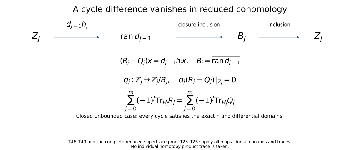
Equations (T46)–(T49) prove the indicated factorization, graph-domain bound and quotient map. Section 6 supplies every induced trace and the reduced-supertrace equality.
Problem 4: an explicit tensor index. Take , the backward shift, and , the forward shift on . Determine the two kernels in (T43), locate the nonzero one in the tensor complex, and compute the index.
Solution. We have , , and . Thus . Of the two odd summands in , the first is zero and the second is , lying in . Hence the index is . The tensor estimate (T45) supplies closed range, so this kernel computation is sufficient here; kernels alone would not establish Fredholmness without that estimate.
Problem 5: spectral compressions without commutation. In Section 5, suppose does not commute with the spectral projections . Verify that the compressed intertwining identity is still valid and explain which domain assertion would be missing if (T18) were replaced by agreement only on an unspecified collection of vectors.
Solution. For , the spectral contract gives . The graph inclusion gives , so is meaningful. Using , and , yields
This is exactly (T20); no interchange of and occurs. Mere equality of formulas on unspecified vectors would not ensure that every is among those vectors or that . The bounded compressed operators could then fail to be intertwined. Graph inclusion is the condition that supplies both requirements.
Problem 6: a trace-class bound without an invalid diagonal-tail identity. Let with Hilbert-Schmidt and let be finite-rank orthogonal projections on the source of with . Prove trace norm convergence of . Must equal the sum of diagonal entries of outside the projection?
Solution. Factor . Then (T7) gives
The proposed equality need not hold. In , take and . The map has trace norm one by (T11). But , whose omitted diagonal entry is . Thus factorization gives the correct approximation estimate even when the chosen projection does not commute with .
12. How trace formulas feed elliptic problems
For an elliptic parametrix, an analytic estimate must first show that appropriate remainder powers belong to the trace ideal. Formula (T28) then converts those analytic errors into an integer. It neither proves the needed trace-class estimates nor requires the original errors to be compact when their powers already meet the hypothesis.
For complexes, cohomological cancellation is a separate mechanism from Fredholmness. Reduced supertraces remain valid with nonclosed ranges, while the parity operator is Fredholm only when closed range and finite-dimensional cohomology are proved. Tensor index multiplication needs the quantitative estimates in (T45); the finite-dimensional kernel formulas by themselves do not supply those range properties.
References
The finite-rank, spectral-compression, reduced-cohomology and tensor proofs are developed here.
The basis, expansion and Parseval part of Hilbert-space geometry can be read as an exact reference import from Mathlib’s Hilbert-basis development, at the displayed commit: exists_hilbertBasis, HilbertBasis.hasSum_repr and HilbertBasis.hasSum_inner_mul_inner. Take the scalar field to be and the space to be complete. The index type is arbitrary. Mathlib’s inner product is linear in its second variable, so its inner y x represents our ; its HasSum gives the finite-subset limit. These declarations cover the named sub-contract, relative to their own imports. They do not supply the other Hilbert-space facts stated in Section 1. The reference code is under Apache License 2.0.
For operator ideals, Jordan Bell, Trace class operators and Hilbert-Schmidt operators, dated April 18, 2016, Theorems 14–19 and 23–25, gives related basis, factorization and cyclicity arguments. Our paired-system norm and finite-rank approximation proofs are given above. Guillaume Bal, Lecture Notes on Topological Insulators, January 15, 2024, Theorem B.4, gives the powers-of-errors formula for operators on one Hilbert space; Section 7 proves it for maps between two spaces.
Jesse Peterson, Notes on operator algebras, April 27, 2020, §4.3.1–4.3.3, provides antecedents for positive closed operators, spectral calculus and polar decomposition. Positive square roots and closed-operator polar decomposition are proved in Lower-bounded selfadjoint operators and their spectral calculus, Section 6, equations (HF6)–(HF17), with the exact domains and spectral-band maps used in Section 1. Their earlier mathematical entry assumptions and the course-wide recursive review remain separately identified.
For the optional measure realization, the countable-cover convention is the primitive product in D. H. Fremlin, Measure Theory, Chapter 25, 251A–251E. The linked results-only version states that convention and carries the Design Science License. Its distinct c.l.d. product should not be silently substituted for arbitrary measure spaces. The abstract tensor theorem does not use this realization.
13. Editorial comparison with Bell’s trace notes
These four corrections concern the original-author TeX of Jordan Bell’s trace notes, April 18, 2016. The theorem statements survive these proof corrections. Sections 1–4 and Problem 6 already give the course’s independent arguments; the notes below identify the precise source passages and prove their repairs.
Theorem 15, right multiplication estimate. The last equality in its right-ideal calculation must be an inequality. With the same original operators and adjoints, the complete calculation is Indeed the left-ideal bound follows by summing over finite basis subsets and taking their supremum; the adjoint equalities are (T1)–(T2). Equality is false in general: on , take , . Then , while .
Theorem 21, a trace tail after projection. For an arbitrary basis projection, its asserted diagonal-tail identity is false. Retain the exact two matrices Their products give The middle matrix is positive and its square is the first, so the square-root uniqueness in Section 1 identifies it. The last positive matrix is its own square root. Thus , whereas the omitted diagonal entry of is .
The density conclusion follows with the original factorization , where are Hilbert-Schmidt. For the projection onto a finite basis subset , retain the ordered product and its actual bound: The norm inequality is (T7), with its two factors identified. The last equality follows because is zero on and equals elsewhere. A finite nonnegative basis sum has tails tending to zero over finite subsets, so (BE4) tends to zero. Each has finite rank. This proves density for arbitrary Hilbert-space index sets, including , without the failed trace-tail equality.
Theorem 22, adjoint polarization. In the first line of the displayed calculation for , the final norm must be . The corrected full polarization is To verify the polarization itself with our first-variable-linear inner product, expand each squared norm of and . Their four weighted terms sum to . The product series is absolutely summable by Cauchy-Schwarz. Summing therefore gives the source’s formula for . Interchanging gives the first line of (BE5). Multiplication by or , of modulus one, gives and , proving the next line. For the scalar operators , the source’s first printed line instead gives , while and . The corrected final norm is zero and (BE5) gives , as required.
Theorem 27, the topology in its final density step. The functionals there have domain , equipped with the operator norm. Their agreement on finite-rank operators extends by density in that norm. Here is the needed proof. For compact and , choose a finite -net in the closure of ’s image of the unit ball. Let be their finite-dimensional span and its orthogonal projection. For every unit-ball vector , choose with . Then The projection has norm at most one, and has finite rank. Given a bounded functional and the trace functional , (T9) and the trace bound proved with (T12) supply . Their agreement on implies Letting tend to zero proves agreement on every compact . This repairs the final step; trace-norm density within alone would not supply it. The zero Hilbert space satisfies the same statement with zero functionals.