From local energy to global divergence equations
A divergence equation can be meaningful before its solution has even one square-integrable derivative. Its positive energy then supplies that derivative, and local elliptic regularity supplies the next one. Global existence has a different difficulty: data may grow arbitrarily towards infinity or the boundary of an open set. We solve that difficulty by assigning a sufficiently large weight to the adjoint residual, with controlled changes on each previously treated compact region.
The argument permits complex coefficients and uses only local Lipschitz bounds. On a manifold it requires a density to specify divergence. We make that convention explicit and separate the existence theorem on noncompact components from the exact obstruction on compact components. No boundary condition or global integrability of the solution is imposed.
1. The equation and the tools used below
Let be a Hausdorff, second-countable manifold without boundary of dimension . An arbitrary open subset of is included. Fix a positive density and a complex symmetric contravariant tensor , with locally Lipschitz coordinate entries. Symmetric means transpose-symmetric, , and does not mean Hermitian. We require
Continuity and compactness make the lower bound uniform on each compact coordinate neighborhood. Since the real and imaginary parts of are real symmetric matrices, (D1) also gives
on that neighborhood. Indeed the imaginary symmetric part contributes a purely imaginary number, and the real part acts separately on the real and imaginary parts of .
In a chart write . Our operator and its Hilbert adjoint on compactly supported tests are
Repeated indices in this lesson are summed from to . The pairing is linear in its first entry. For Euclidean Lebesgue density, (D3) is , with , as in Local inverses and distance-weighted elliptic estimates.
For , the equation means
This pairing is defined: is a bounded, compactly supported measurable function. In each chart (D4) agrees with distributional differentiation. More explicitly, for a Lipschitz multiplier , define
The right side belongs locally to . Multiplication by and changes of charts in (D3) can be interpreted through (D4); no product of an arbitrary second-order distribution by a merely function is being postulated. The equivalent chart equation is .
There is no need to choose an unmentioned smooth structure. Compactly supported tests suffice for an operator of order two acting on . In a coordinate chart, approximation in shows that an equation against smooth tests also holds against these tests. Finite partitions of unity make the equivalence global. The coordinate changes are ; their first derivatives and inverse first derivatives are bounded on compact subcharts, and their second derivatives are bounded there. The ordinary chain rule, first on smooth functions and then by Sobolev approximation, therefore preserves local and . The transformation of uses first derivatives of the coordinate map, so its new entries remain locally Lipschitz. The density has the usual absolute-Jacobian transformation. These facts make (D3) and (D4) intrinsic, including on a nonorientable manifold.
The following dependencies specify the base of the proofs.
- Weak Lipschitz products. Section 7 of Local inverses and distance-weighted elliptic estimates gives the weak Lipschitz product (D5) and the Friedrichs commutator bound, including convergence, on .
- Weak elliptic regularity. Section 8 of Local inverses and distance-weighted elliptic estimates proves that for a second-order elliptic principal operator with locally Lipschitz complex coefficients, and imply , with the local estimates proved there. Its quantitative estimate comes from Section 6 of Local inverses and distance-weighted elliptic estimates.
- Support continuation. Sections 7–8 of Curved weights and the directions in which support can end prove continuation from a nonempty open subset of a connected domain for an solution satisfying , when every normal is admissible. Positive real part gives this admissibility also in dimension two: the path , , remains elliptic and preserves the number of roots in each half-plane. No reality assumption at a point is needed in this positive-real-part case.
- Sobolev and compactness facts. The local and weak-derivative calculus, smooth approximation in integer Sobolev spaces, boundedness of convolution on , weak subsequential compactness of bounded Hilbert-space sequences, and compactness of bounded sequences in , or bounded sequences in , when their supports lie in one fixed compact interior region. The compactness statements transfer through a finite collection of charts. A weakly differentiable function with zero gradient on a connected open set is almost everywhere constant.
- Manifold geometry. Locally finite partitions of unity and compactly supported cutoffs on second-countable manifolds; a positive density and a auxiliary Riemannian metric exist. Only their local coordinate bounds are used. A manifold is locally path connected and locally compact; its connected components are open, and each connected component is path connected. The compact-hull construction needed below is proved in this lesson.
- Hilbert-space tools. The complex Hahn–Banach theorem for a bounded linear functional on any linear subspace of a normed space, and the Riesz representation theorem for bounded linear functionals on a Hilbert space. The extension in the global proof is generally from an infinite-dimensional subspace; a finite-dimensional extension contract would not suffice. We also use completeness, the Cauchy–Schwarz inequality and the convergent geometric series for an operator of norm less than one.
The Hilbert-space tools have complete proofs in this course. Section 5 of Banach estimates, quotient spaces and compact parameter arguments proves norm-preserving complex Hahn–Banach extension from any linear subspace, including one that is neither closed nor finite dimensional. Section 2.3 of Spectral measures with the original operator domain retained proves Hilbert representation with the linear-first convention; Section 6.5 proves the operator geometric series and both inverse products. These proofs supply exactly the functional extension, represented vector and inverse used below.
The argument uses these stated entry results and the named prior lessons. No global solvability theorem is assumed.
2. Energy recovers the first derivative
Local gain. If and , then .
We first work in a Euclidean chart and multiply the equation by . Set and . The entries of are Lipschitz and their real part is uniformly positive on any fixed compact subchart. A multiplier acts boundedly on local : by duality its action is the product on , where the first-order product rule gives the bound. Thus .
Choose a smooth cutoff supported in the chart. Distributional product rules, using (D5), give
All terms on the right belong to after zero extension. For the last term put and write . Both and are with fixed compact support. The same observation justifies the product rule itself by local smooth approximation of in .
It therefore suffices to treat supported in a compact set inside the chart, with . Extend the coefficients by a cutoff on a slightly larger chart; they become globally Lipschitz and agree with the original positive matrix on a fixed compact neighborhood of . Positivity of the extension outside is irrelevant.
Let , where has integral one. For small , is smooth with support in . Define the vector commutators
The bound is exactly Section 7 of Local inverses and distance-weighted elliptic estimates, applied to each entry and derivative; replacing by only multiplies by a scalar of modulus one. Hence
In particular no derivative of a Lipschitz coefficient of order two has appeared. Choose a fixed box containing . The elementary compact-support Poincaré estimate follows by integrating along lines parallel to one coordinate axis from a face of that box, where its zero extension vanishes, and applying Cauchy–Schwarz. Integration by parts and (D2) now give
If the last norm is zero there is nothing to divide by; otherwise cancellation gives a uniform bound. A sequence has a weak limit. Its strong limit is , so uniqueness of distributional limits identifies the weak limit with . This proves , and (D6) proves the local assertion. The argument also yields, for nested compact subcharts,
where and the local negative norm is taken after a fixed cutoff equal to one near . A finite chart cover supplies the same statement on .
3. The second derivative and the local estimate
Regularity theorem. Under (D1)–(D3), if satisfy (D4), then .
By Section 2, . In a chart the weak product rule gives
The parenthesized coefficients are locally bounded. Its right side is now , and the left side is the weak nondivergence principal operator of Section 8 of Local inverses and distance-weighted elliptic estimates, with . The real part of its principal symbol is positive in the sense (D1), so it is elliptic. That result gives , with no differentiability of the first-order coefficients beyond boundedness. Its quantitative local estimate yields
using finitely many nested coordinate neighborhoods when necessary. Here and below Sobolev norms on relatively compact regions may be defined using any fixed finite chart partition; the choices give equivalent norms. Applied after (D10) on a slightly larger region, (D12) also gives the familiar interior estimate with on that larger region. The proof has established finiteness of before using (D11), and finiteness of before applying any estimate to its highest derivatives.
There is a useful support-preserving approximation consequence. If has compact support inside an open set , then there are , supported in one fixed compact subset of , with
To construct them, choose a finite partition near , subordinate to coordinate charts compactly contained in . Each partitioned function has compact support in its chart. Convolve its zero extension there and take the sum after returning to . The margin between the supports and chart boundaries keeps all approximants in . Chartwise mollification converges in , and multiplication by a cutoff is bounded on . Finally (D3) expanded as in (D11) defines a bounded map from to on that fixed compact region. This proves the second convergence. The same statement holds with .
4. Fixed-support coercivity and continuation
For the next three sections assume that every connected component of is noncompact. No uniform ellipticity constant on all of is required.
For a fixed compact , choose a relatively compact neighborhood of . Every supported in satisfies
Here is measured by an auxiliary metric and the norm can be computed within . For a proof, failure would give supported with and . This sequence is bounded in . Compactness on a finite chart cover gives a strongly convergent subsequence with limit , of norm one, supported in , and with weak gradient zero. On every connected component it is constant. A component has points outside , since it is noncompact; near such a point the supported function is zero. Thus every constant is zero, a contradiction. A compact set meets only finitely many components because those components form an open cover of it. This also justifies the finite chart argument if is disconnected.
The energy identity extends by approximation from tests to supported functions:
When the first entry is in , the pairing in (D15) denotes its dual action. Combining (D14) and (D15), and defining the negative norm by duality with , gives
The last inequality is used only when . For compactly supported tests, (D12) and (D16) imply
The constants depend on a compact neighborhood of , its coefficient bounds, and the fixed norm conventions. Formula (D17) is precisely the compactness bound needed in the global construction.
The second ingredient is support propagation. If , is connected and open, and , then vanishing on a nonempty open subset of implies throughout . Indeed (D11), conjugating the principal coefficients, gives on every compact subchart. Its principal form has positive real part. Section 8 of Curved weights and the directions in which support can end verifies every normal using the positive-real-part path, and Section 7 of Curved weights and the directions in which support can end gives continuation. These are local statements, so coordinate neighborhoods propagate the conclusion along any path in . This checks the complex coefficients and the density term in the exact use of unique continuation.
5. Filling the bounded complementary components
For a compact set , define its filled hull by adjoining every connected component of whose closure in is compact:
We retain the assumption that has no compact connected components. Then is compact, and has no relatively compact connected component. We prove compactness rather than impose it as a further geometric condition.
Choose a relatively compact open neighborhood of , with . Such a neighborhood is a finite union of precompact chart neighborhoods. Its boundary is compact and disjoint from . Cover by finitely many connected open neighborhoods disjoint from . Each lies in one component of , so at most components of that complement meet .
If a component is relatively compact, the ambient connected component of containing it must meet . Otherwise , contradicting the noncompactness of . If also , choose and join to a point of by a path in . Up to its first meeting with , the path remains in . It must cross before meeting , since . Thus is among the finitely many components just found. Consequently every component added in (D18) is contained either in or in one of finitely many relatively compact components. Their closures together with form a compact set containing .
The hull is closed: its complement is the union of the other components of , each open by local connectedness. Therefore the hull is compact. Those remaining components are exactly the components of its complement and none is relatively compact, by their selection. Notice that need not have a smooth boundary, finitely many boundary components, or even nonempty interior.
We obtain a sequence of compact sets
Indeed choose a countable cover by precompact coordinate neighborhoods. Given , enclose it and the closures of the first members of the cover in a precompact open set , and set . Start in the same way with the first neighborhood. The hull contains , so lies in its interior. The countable cover proves exhaustion. This construction uses no regular-value theorem and preserves the setting.
6. Extending an adjoint weight without disturbing the interior
Fix and an exhaustion (D19). Write for the functions supported in . Suppose and a continuous positive function on satisfies
For every there is a continuous positive such that
Proof. Choose , , equal to zero on a neighborhood of and equal to one outside . Set
If no satisfies the last line of (D21), choose a violating . Its pairing with is nonzero; multiply it by the reciprocal of the conjugate of that pairing to arrange
The positive minimum of on gives a uniform bound for . Formula (D17) then bounds in , all with support in that same compact set. Pass to a subsequence weakly convergent in and strongly in , with limit . The limit has support in , and , since is square integrable there. The bounded coefficient formula for on a compact neighborhood gives weak convergence of to . Since is bounded on that neighborhood, weak lower semicontinuity gives
On , (D22) and (D23) give
Thus on . Every component of this open set is not relatively compact. It cannot be contained in the compact set ; hence is a nonempty open set. There . Continuation from Section 4 gives throughout . This establishes
One must use continuation from an open zero set at this point: need not have compact support relative to , since its support may approach .
Since , approximation (D13) gives converging to in . It also gives in , because is bounded on the fixed approximation support. Passing to the limit in (D20) yields
which is impossible. At least one therefore works; take it as .
The argument explains the two inner compact sets in (D21). The weight remains controlled on ; the limiting adjoint solution is supported in ; the extra margin to permits approximation in the previously proved estimate.
The weight step when compact components are present. The implication (D20)–(D21) holds on any manifold satisfying (D1)–(D3) with an exhaustion (D19), even if compact connected components are present. A filled exhaustion does not itself exclude them. Each compact connected component must lie entirely in : otherwise a component of would be a relatively compact component of , contradicting (D19). There are finitely many such , because they all meet the compact set and the components of are open. Their indicator functions belong to . Testing (D20) with shows that .
For any test , replace it by
For every , this operation preserves , the residual , and the pairing . Its image has mean zero on each compact component. The proof of (D14) applies to supported functions in this image: a limit with zero gradient is constant on each component, vanishes on each noncompact component by its support, and vanishes on each compact component by its mean. Therefore (D16)–(D17) hold for these projected functions. In the contradiction argument, project each violating test before imposing (D23). The projection leaves both quantities in (D23) unchanged, and its mean-zero conditions pass to the weak limit. The remaining steps (D24)–(D27) are unchanged; in particular, (D19) supplies the same nonempty open zero set on every complementary component. This proves the weight extension in its full filled-exhaustion setting. It does not construct an initial estimate for data of nonzero mean on a compact component.
7. Global existence on noncompact components
Solvability theorem. Assume (D1)–(D3) and that every connected component of is noncompact. For every there exist a continuous function , a function with , and satisfying .
Construction of the weight. By Cauchy–Schwarz and (D16),
Thus a positive constant function larger than the last coefficient establishes (D20) for . Choose positive numbers , , with , for example . Inductively use Section 6 to obtain from . Put
The positive numbers increase to a finite : use for . Moreover everywhere and on . On any fixed compact neighborhood this sequence is therefore eventually stationary. Its limit is continuous and positive, since locally it is exactly one of the continuous positive functions . Set . Equivalently, locally uniformly: after stationarity, only the scalar is changing. In particular , and every compactly supported test belongs to for some . We have proved
Dual construction of the solution. Let be the linear subspace of consisting of the vectors , . Define a complex linear functional on it by
If two tests give the same vector in , their difference has zero right side in (D30), so (D31) is well-defined. Also . Hahn–Banach extends to with norm at most one. Riesz representation gives , , such that . Conjugating (D31) now gives the correct pairing order:
Since is locally bounded, belongs to ; (D32) is its equation (D4). Section 3 supplies . The earlier sentence that differentiation of was not justified was too weak: the actual recursion gives a twice continuously differentiable weight, as the separately identified strengthening in Section14 proves. Regularity comes from the equation, even though the weight itself was only continuous.
The theorem gives existence for each datum. It does not assert uniqueness, a globally bounded inverse on unweighted , a solution satisfying prescribed boundary values, or a datum-independent choice of . These distinctions matter when this theorem is used as a local ingredient in a boundary or Fredholm problem.
8. The exact compact-component obstruction
The local regularity theorem applies on compact manifolds too. The unrestricted global existence assertion does not: on a compact connected component , the test has compact support in and . Thus a necessary condition is
For the pure divergence operator (D3) this is also sufficient. We include the proof to identify the entire obstruction rather than merely give a counterexample.
Let be the closed subspace of with mean zero. On the gradient norm is equivalent to the full norm. Indeed failure of Poincaré would give a normalized sequence converging strongly in to a constant of mean zero, exactly as in the proof of (D14), a contradiction. Define
Its boundedness follows from the bounded coefficients on . Its real part satisfies for some . Fix any Hilbert norm on equivalent to , with pairing linear first. Riesz representation in the second entry supplies a bounded operator with . Let , where . For ,
Thus has norm less than one (possibly zero), and the geometric series gives an inverse for . The bounded conjugate-linear functional on is represented by a vector . Solve ; then for every . Any test differs from an element of by a constant. Both sides vanish on constants, the right side by (D33). Hence on , and Section 3 gives .
If on , local regularity and compactness give whenever . Its energy is zero, so (D2) implies ; it is constant. The same proof applies to . Consequently the adjoint obstruction is exactly the constants on each compact connected component, and the normalized solution there is unique.
We have proved the following complete form for a possibly disconnected manifold:
For sufficiency solve separately on compact components by (D34)–(D35), and on noncompact components by Section 7. There are at most countably many components by second countability. Every compact subset meets only finitely many of them, so their componentwise solutions assemble to an function. Necessity was (D33).
For Euclidean open sets no component is compact, so (D36) gives arbitrary-data solvability without an additional condition. For the manifold formulation, the noncompact-component convention or the obstruction in (D36) must be stated. An unqualified assertion of arbitrary-data solvability on every boundaryless manifold would be false, even for the Laplacian. This is a mathematical qualification of that formulation, independent of any unstated convention in a reference.
9. Worked models
Example 1: a complex Lipschitz coefficient and rapidly growing data. On , take
The real part of is at least two, but is not differentiable at zero. Define
These integrals are finite on every compact interval. Since is continuously differentiable and is locally Lipschitz, is locally Lipschitz and . Its flux is , so differentiating once gives , including across zero. No pointwise value of is required. Arbitrary constants may be added both to and to , producing the two local homogeneous degrees of freedom. The theorem accommodates the growth of because it asks for local, rather than global, square integrability.
Example 2: bounded in coordinates need not mean relatively compact. Let and . Its inner complementary component is bounded in but is not relatively compact in : a sequence tending to the missing origin has no convergent subsequence in . The outer complementary component is also not relatively compact. Thus in this manifold. The distinction explains why the support argument is expressed intrinsically, with compact closure in , rather than by a Euclidean size test. For any later compact , the inner component has points outside , as the continuation step requires.
Example 3: mixed compact and noncompact components. Let , use the standard densities, and choose on both components; both torus coordinates have period . Give the plane the datum , and the torus the datum . A solution is
Each is locally ; direct differentiation verifies the equation. Replacing by makes its integral nonzero and destroys solvability on that component, while the plane equation remains solvable. A compact-component obstruction is a condition on that component’s datum, not on the behavior at infinity of other components.
10. Problems and full solutions
Problem 1. On the line let and . Compute as a distribution. Verify that its local regularity is compatible with Section 2 but does not trigger Section 3.
Solution. Almost everywhere , and . Since the distributional derivative of is ,
The Dirac mass belongs to . For instance, for a smooth compactly supported , integrate from an endpoint beyond its support to zero; this gives . Evaluation therefore extends continuously to . Thus (D40) has the negative regularity needed for the first gain. In fact . But is not represented by an function, so near zero. The datum in (D40) is likewise not . The two stages of the theorem have different data assumptions, and this example distinguishes them.
Problem 2. Start with , Lebesgue density, and the coordinate change . Determine the transformed density and tensor coefficient and check the first-order term of the transformed operator.
Solution. Write . Since , this is a global smooth coordinate change. The density and coefficient are
Thus , with the right side evaluated at . The divergence formula gives
Here . The same result follows from , applied twice. If the density were omitted and one wrote , the first-order coefficient would instead be , giving a different operator. This is why a divergence formula with coordinate-dependent coefficients needs its density convention.
Problem 3. For a fixed real , consider on the form . Check the normal-root condition for , then explain why it holds for every real normal without choosing roots continuously over all normals.
Solution. For the line polynomial is . Its two roots are opposite, nonzero numbers. Neither is real, since a real would give real part . Hence one lies in each half-plane and the roots are distinct. For arbitrary independent real , use , . The leading coefficient is nonzero and the line polynomial has no real root throughout the path. At its real coefficients yield a nonreal conjugate pair. Continuity of the unordered pair of roots preserves the number in each half-plane, so the same is true at . When is parallel to , the root corresponds to the zero argument and is excluded from the normal criterion. The path argument is pointwise in the chosen pair and requires no global root labeling.
Problem 4. Determine solvability of on if the desired solution is (a) locally , (b) globally . Compare with the same equation on the circle. Explain what the global theorem actually supplies.
Solution. Integrating distributionally twice gives every solution on the line as , where . These functions are smooth and therefore locally . None is globally : its quadratic leading coefficient cannot be canceled by the affine part, so for sufficiently large , . On the circle, integration against the constant test gives , an impossibility. Thus arbitrary-data local-Sobolev existence on a noncompact component gives neither unweighted global integrability nor arbitrary-data existence on a compact component. In the weighted representation , one may have precisely because the allowed grows; boundedness of was never asserted.
Problem 5. In the weight construction, replace by , . Show why the argument no longer produces a finite continuous weight on the previously treated interior. Does this refute the solvability theorem?
Solution. On every step satisfies the exact equality , since . Hence there
The initial weight is strictly positive, so this tends to infinity at every point of . Normalized weights still stabilize there, but the compensating scalar product does not have a finite limit. The argument therefore needs a bounded product of interior enlargement factors, supplied by summability of the positive . This failure concerns that choice of iterative construction. Choosing the summable sequence used in Section 7 proves the theorem and avoids the divergence.
Problem 6. Explain concretely why one cannot replace the filled exhaustion by an arbitrary compact exhaustion in the continuation step. Use the Laplacian on and a compact annulus.
Solution. Take and a smooth radial function equal to one on and zero on , with its transition strictly between these radii. Then . Thus on , and has compact support. But is nonzero on the bounded complementary component . Continuation does not force zero there, because there is no nonempty open zero set within that connected component. The support conclusion would be false. Filling the inner disk replaces by , for which the support conclusion is correct. The failure occurs in the support inference, not in local regularity or the energy estimate.
11. The manifold geometry used by the equation
We prove all the geometry used in Section 1 on its original Hausdorff, second-countable manifold without boundary and of dimension ; the notation below retains those original objects. If is empty, the empty partition has sum one at every point vacuously, the unique empty metric and density have all the stated positivity and regularity properties, every compact subset is empty and has zero cutoff, and there are no components. All the assertions therefore hold in that case. For the remaining construction assume is nonempty. The proof uses the original coordinate compactness and finite scalar calculus; it does not select a smoother atlas.
11.1. Countable compact exhaustion from the original charts
Every point has a coordinate neighborhood and a smaller coordinate ball whose closed ball is contained in the coordinate image. Its inverse image is compact, since the inverse chart is continuous and the closed Euclidean ball is compact. It is closed in , since is Hausdorff. Its interior is an open neighborhood of the point. This proves local compactness and gives an open cover by relatively compact coordinate balls.
Here is the countable-subcover argument used in the construction. Fix the given countable topological base. For each base member contained in some member of the cover, choose one such cover member. This gives at most countably many chosen members. Any point of the covered space belongs to a base neighborhood contained in a cover member, so belongs to one of the chosen members. The chosen family covers . This argument applies to every open cover, with no countability assumption on that cover.
Write the resulting relatively compact coordinate balls as , allowing a finite list when it is finite. Put . Choose . Given compact , cover it by finitely many relatively compact coordinate balls and take the union of their compact closures together with the compact closures of the first members of the original cover. Call this finite union . It is compact; the open balls covering show . Including the first original balls makes the interiors exhaust . In a finite cover, include every available member once the index exceeds its length; the same construction works, and may become constant at if is compact. Thus There is no connectedness requirement. Each compact subset of lies in the interior of some , by a finite subcover of these increasing interiors.
Define the original compact shells and their open neighborhoods by The shell is compact, and : it lies in , while makes it disjoint from . Every point lies in some shell, by choosing the first index for which it belongs to .
11.2. Compactly supported partition subordinate to any open cover
Let be the original open cover. For every point of , choose a coordinate ball with closed outer ball inside , inside one assigned member , and inside its original chart. Choose concentric coordinate balls of radii , with the closed radius- ball inside this open intersection. The radius- balls cover ; compactness selects finitely many, indexed by . Denote the smaller balls by and the radius- balls by . The chosen finite families together cover , and . Empty shells need no balls.
This family is locally finite. If , that same open set is a neighborhood meeting none of the with , because their ’s exclude . Only finitely many shells remain, and each has finitely many balls. This proves local finiteness on the original space, rather than assuming a paracompactness theorem.
To construct the needed coordinate functions, put For , each derivative of is a finite polynomial in times , by induction using the product and chain rules. Every such expression tends to zero as : for each positive integer , the exponential series gives , and choosing larger than the polynomial degree proves the limit. Thus extension by zero makes smooth with all derivatives zero at zero. The denominator in (MG3) is positive for every real ; is smooth, equals zero for , equals one for , and lies between zero and one.
In the original chart of a selected ball with center and small radius , define It equals one on the closed radius- ball, and is zero outside the radius- ball. Its support is compact inside . Composing with the chart and extending by zero gives a function on : the support has an open neighborhood inside the chart, and the function is identically zero near every point outside that compact support. This retains the manifold’s structure and introduces no unmentioned smoother atlas.
Let denote these countably many indices and put Each sum is a finite sum on a neighborhood of each point by local finiteness. The inner balls cover , so . The quotient is therefore . The ’s are nonnegative, their compact supports stay in the original assigned cover members, and their family is locally finite. Their exact derivatives in any original chart are All sums and all denominator factors remain present. On a compact subchart only finitely many supports meet the compact set, so every derivative through order two has a finite supremum there. This proves precisely the subordinate locally finite partition asserted by the original contract.
11.3. The original compact cutoff and positive local-radius minorant
If a compact lies in an open , apply the partition construction to the cover . A locally finite family meets a compact set in only finitely many members: cover the compact set by finitely many neighborhoods each meeting finitely many supports. Take the finite collection of supports assigned to that meet , and define . Then , , and its support is contained in the finite union of the selected original compact supports.
In fact on a neighborhood of , not just on . Every unselected support is disjoint from : a support assigned to is contained there, and every other support disjoint from was not selected. A locally finite union of closed sets is closed, because near each point that union is a finite closed union. The union of the unselected supports is therefore closed and misses . Its open complement is a neighborhood of ; there every unselected vanishes, so (MG5) gives . If , use . This proves every required compact cutoff.
There is also a useful proved consequence for the local radii used in the continuation and kernel constructions. Let have a positive lower bound on some neighborhood of every point, as does a positive lower-semicontinuous function. Choose such neighborhoods , with constants for which on , and take the proved subordinate partition, assigning each support its original . Then The sum is locally finite and , and at least one positive summand occurs at every point. Each term active at has , and summing with (MG5) proves the upper bound. No positive global lower bound or compactness of is assumed.
11.4. Positive metric and the exact density transition
Take a locally finite partition as above subordinate to the original coordinate neighborhoods. In each such neighborhood with coordinates , retain the coordinate metric . Its coefficients in another chart are , since The chart derivative is invertible: the chain rule for the original chart and its inverse gives both inverse matrix products. Hence for every nonzero real tangent vector in that neighborhood.
Extend each by zero and define . The compact support inside its chart makes each extension ; local finiteness makes the sum . At a point and a nonzero tangent vector, some is positive and its is positive, while all other terms are nonnegative. Thus is a positive Riemannian metric on the original manifold. It need not coincide with any metric already chosen in the divergence equation.
Write its matrix in coordinates as , and keep the full density The determinant is a finite polynomial in the matrix entries. It is positive for a positive real symmetric matrix: the real spectral theorem gives positive eigenvalues whose product is the determinant. The ordinary scalar square root is on the positive axis, so the coefficient in (MG8) is positive and .
On an overlapping original chart , put . The tensor chain rule gives , including both matrix factors in their displayed order. Taking determinants yields This is exactly the density transition factor. It patches the coefficients in (MG8) to a density, including orientation-reversing changes of coordinates and nonorientable manifolds. No sign of a determinant is chosen or discarded.
Every compact subchart has positive finite lower and upper bounds for this density coefficient, and finite bounds for its first derivatives. For the metric, the continuous function on the compact subchart times the original Euclidean unit sphere has a positive minimum and a finite maximum; its coefficient first derivatives also have finite suprema. These are precisely the local bounds used by the divergence chapter. The constructed density proves existence; the original separately fixed positive density in (D3) is retained, and is not silently replaced by . The same compactness argument gives local bounds for that original positive coefficient.
11.5. Components and exact receiving scope
Coordinate balls are path connected: the inverse chart applied to the straight segment in the original ball gives a path between its points. They form a neighborhood base. Thus is locally path connected. Local compactness was proved in Section 11.1.
A path component is open: any point in it has a path-connected coordinate ball, and concatenation of its path with paths in that ball places the whole ball in . The other path components are open for the same reason. A path is connected, because any separation of its image pulls back to a separation of the interval; the interval’s connectedness follows from completeness and the intermediate-value theorem. Consequently a path component is connected: it is the union of the connected images of paths through its fixed point, and a union of connected sets sharing that point cannot be separated.
The connected component through a point contains its path component. If it contained a second path component, its intersection with the first and with the union of the others would be a separation into two nonempty relatively open sets. This is impossible. Thus each connected component equals a path component, is open, and is path connected, exactly as the original contract states.
These proofs supply the geometry entry needed for the finite chart arguments in (D4)–(D10), the compact cutoff in the energy proof, the local metric and density bounds, the connected component alternatives and the exhaustion/partition steps in the global divergence construction. Section 12 separately proves nonlinear substitution for the completed coordinate measure and the exact weak Sobolev chain maps under the original coordinates, together with their receiving density and adjoint formulas. The original contract’s statement and the original , , operator signs and Hilbert pairing are unchanged.
For a manifold, integer , this same proof gives partitions, compact cutoffs and local-radius minorants, and a positive metric and density. Every transition calculation uses exactly one derivative of the original chart; every other step preserves its regularity. For a smooth atlas this same construction is smooth at every order; local finiteness makes every derivative a finite sum.
12. The exact coordinate maps in the weak equation
The geometry in Section 11 supplies the original charts and cutoffs. This section supplies the analytic maps asserted in Section 1. Throughout, , is a diffeomorphism between the original open subsets of , , and The chain rule for the two actual inverse maps proves both matrix products and the full determinant identities: No orientation is chosen. Empty chart domains give empty maps and zero integrals; below the domains are nonempty.
12.1. Substitution for the completed original coordinate measures
The completed-measure substitution theorem also has a full proof for C¹ diffeomorphisms in Singularities along a submanifold, Section 16.9. The argument below is an alternative proof using contraction on each original cell. The C² coordinate assumption enters the later second weak derivatives; the measure argument uses only C¹ regularity of both inverse maps. Its identity then enters the weak derivative, density, tensor and weak equation calculations in Sections 12.2–12.4.
We first prove the measure identity, rather than assume nonlinear substitution in a Sobolev approximation argument. An invertible real matrix acts on the original completed coordinate measure by Here is a proof retaining the actual matrix factor. For a coordinate shear , with , fix the other coordinates. Every one-dimensional section is translated, so its length is unchanged. Integration of these sections, first for nonnegative Borel indicators, proves preservation of measure. A coordinate permutation preserves iterated product measure; reflection preserves length; multiplication of one coordinate by a nonzero scalar multiplies length by . One-dimensional length has these properties directly from the original interval lengths and their completed-measure uniqueness. Gaussian elimination expresses every actual invertible as a finite ordered product of these invertible elementary matrices: at column , choose a nonzero pivot in the remaining rows (failure would make the remaining columns linearly dependent), exchange its row with row , divide that row by the nonzero pivot, and subtract its multiples from every other row. After steps the actual product is . Thus , in that order. Applying the preceding section calculations successively multiplies measure by . Every elementary factor and the determinant of the original are present in this comparison.
A map with Lipschitz constant in the coordinate maximum norm sends null sets to null sets on any cube on which that bound holds. Indeed a cube of side maps into a cube of side , by centering at its center and bounding every image coordinate by . A null subset has cube covers with total original volume as small as desired; the image outer measure is at most times that total. Cubes in these covers can be taken within a slightly larger fixed cube contained in the domain: intersect with the interior region and subdivide into sufficiently small dyadic cubes before taking the cover. Thus the bound applies to every covering cube. A map is Lipschitz on a closed cube compactly inside its domain, by integrating its derivative on the segments of that cube and using the maximum row-sum matrix norm. Such cube interiors have a countable subcover of the domain. This proves local null-set transport for , and for , including both directions. In particular the images of all coordinate cube faces have measure zero.
Fix a closed cube , and subdivide it into congruent small cubes , of side and centers . Their images meet only along images of faces, since is injective. Put . The inverse matrices have a uniform finite maximum row-sum bound: the cofactor formula has a nonvanishing determinant on the compact cube. Uniform continuity of gives numbers , such that on each cell In the following calculation retain and explicitly. Define the exact error Then , its Lipschitz constant on is at most , and . Hence For the reverse inclusion suppose , and fix . The map sends the closed original cell to itself and contracts distances by . Starting at any point, its consecutive differences are bounded by a geometric sequence. Completeness of the closed cube gives a limit; continuity gives a fixed point, and the contraction estimate makes it unique. At that point . Thus These inequalities use (CX3) with the entire original derivative matrix. Summing over the cells is valid because their boundary images are null. The continuous function has Riemann sums tending to its integral on : upper and lower step sums differ by at most its uniform oscillation times . Both factors and tend to one. Therefore
For completeness this cube calculation determines the full Borel measure. Define on Borel subsets of , and . The homeomorphism makes images Borel, and injectivity makes countably additive. Both measures are finite on compactly contained cubes and give zero measure to all dyadic faces. Every open subset of is covered, off the countable union of those faces, by disjoint interiors of dyadic cubes with closure in . To see this without a maximal cube at infinity, take integer levels . At level , choose all cells whose closure lies in and whose interior has not already been selected at a preceding level. Dyadic nesting makes their interiors disjoint. Every point off the faces eventually lies in such a cell, because its distance from the complement is positive in some small neighborhood. Equation (CX5) and countable additivity show .
Equality on open sets implies equality on Borel sets here as follows. Both measures are regular on a relatively compact open . For , transport compact inner approximation and open outer approximation for the original coordinate measure through the homeomorphism . The image is bounded after replacing by a relatively compact cube interior, so these approximations concern finite measure. For , is bounded above on the closure of that cube: the error of a coordinate-measure open or compact approximation is bounded by that supremum times the original measure error. Restricting to a cube interior gives regularity there for both measures. For a Borel subset of that interior, the outer approximating relative open sets have equal measures for and ; taking their infima gives equality on . Cover by countably many relatively compact cube interiors, disjointizing that cover by removing the preceding members. The resulting Borel pieces remain subsets of individual interiors, so countable additivity gives equality for all Borel .
The previously proved null-set transport extends this equality to the completed coordinate measures: a completed-measurable set is a Borel set modified within a Borel null set, and its image has the corresponding Borel image and null modification. The inverse map gives the converse. Approximating nonnegative measurable functions by simple functions, and then using monotone convergence, proves the exact original substitution law for every nonnegative measurable , allowing . Applying it to gives equivalence of absolute integrability; the real and imaginary positive/negative parts then prove (CX6) for complex integrable . The analogous identity for retains . Null sets in either chart are null in the other, so all compositions below are well-defined on actual almost-everywhere equivalence classes.
12.2. The full first and second weak derivative maps
Let , with the original complex-valued weak derivatives, and . For classical functions the ordinary chain rule gives every term in The second sum is essential on the original charts. With the original the exact version is No second derivative of , mixed term, or factor is suppressed.
Here are complete local bounds, including the original array multiplicities. For , put , , and Use the full original integer norm , . Substitution with gives . Apply this inequality to every summand in (CX8), and use that each original component norm is at most the full original array norm. Summing the squares over and over , which includes each multiindex of order two exactly once, proves Within each , the entire ordered sum over remains present, including both occurrences of a mixed derivative when its two indices differ. The norm on the left retains the original unordered multiindex count. These are bounds, not a replacement of either array.
To prove the weak assertion, choose a coordinate cutoff equal to one on a neighborhood of . The elementary Euclidean cutoff follows from the flat scalar function in (MG3), or from a finite sum of coordinate ball cutoffs. The full product rule is It holds weakly by the proved integration/product rules of Section 15 in Banach estimates, quotient spaces and compact parameter arguments. The zero extension of belongs to : it vanishes on an open neighborhood of the chart boundary, so integration against a global test introduces no boundary term. Original mollifiers give in the full norm, by that lesson’s support-preserving derivative and translation estimates. Each is smooth; its pullback is . Apply (CX9) to the differences on . These pullbacks and both displayed derivative arrays converge in . Integration by parts against any smooth compactly supported test passes to the limit, proving (CX7)–(CX8) for . The same proof with only first derivatives gives the assertion; order zero is exactly (CX6). The inverse map has the identical proof with replaced by the actual . Both compositions are the identity on the actual local equivalence classes, by (CX2) and null-set transport. Thus the original and chart spaces and their supports agree through the exact maps.
There is an exact negative-order map as well. For a local scalar distribution , define its scalar coordinate representative by The right-hand test is compactly supported , and is admissible through the extension of . Multiplication by any coefficient on the compact support is bounded on : the full rule gives the bound with squared coefficient Together with (CX9) for , this bounds (CX10) on each compact subchart and proves . The test map has compact support and is the limit of smooth compact tests by the same cutoff and mollifier construction; hence it lies in the actual test domain. For an representative , (CX6) shows that , with precisely the factor in its action. Applying the inverse test map introduces and ; their full product in (CX2) is one, so the two distribution maps are inverses. A density-valued distribution instead transforms by ; this second map also is bounded on , but has a different test formula. The scalar and density-valued maps have both been constructed rather than identified by dropping a determinant.
12.3. The original density and contravariant tensor in the equation
Keep the density and coefficients fixed in (D1)–(D3), rather than substitute the auxiliary metric density. Their exact coordinate transforms are The first is positive , because is , the original is positive , and its nonzero determinant has locally constant sign. Each tensor entry is locally Lipschitz: and are and have bounded derivatives on compact subcharts, and the original entries are locally Lipschitz. To check this directly, subtract a product at two points as Every summand has one Lipschitz difference and two bounded factors. Sum this identity over the original entries in (CX11); it retains every factor and proves the assertion.
The original transpose symmetry is preserved by the ordered product . For a real nonzero covector in the chart, the real vector is nonzero by (CX2), and On compact subcharts the minimum of on the original unit sphere is positive. Thus an original local lower bound transfers to times that actual minimum. The density factor is still separate.
For , write , . The scalar substitution law, full chain rule and (CX11) give the entire energy equality In the last step the factors and form the original transformed density exactly. Neither a tensor derivative term nor a density factor was discarded.
Integration by parts in the original charts, which is valid for locally Lipschitz coefficients and compactly supported tests by the proved weak product rule, identifies the left side of (CX13) with , and the right side with . After substitution this proves Indeed both sides are bounded and compactly supported on the relevant subcharts; testing their difference against all forces that difference to vanish. Such tests include every smooth compactly supported coordinate test; the positive density may be divided out using its local lower bound and the density of those tests. Every is for , so no test class was omitted.
For an arbitrary original , put , . Equations (CX6) and (CX14) give the exact receiving identity Thus the original weak equation (D4) holds in one chart precisely when it holds in the other. This proves the original intrinsic operator and its actual test domain without multiplying an arbitrary second-order distribution by a function. For , the same equality follows from (CX13) by the proved approximation and energy bounds; the scalar negative-order map is exactly (CX10). Orientation-reversing charts retain the absolute determinants throughout.
12.4. Gluing the actual measures, supports and finite chart norms
The positive density now defines a completed measure on the original manifold. Choose the locally finite coordinate partition proved in Section 11. In chart with coefficient , set for a Borel Each summand is a Borel measure, and nonnegative countable sums preserve countable additivity. In any one chart, apply (CX6) and (CX11) to the intersections with . Each summand becomes the integral there of , with its full absolute determinant. Summing and using the locally finite identity proves that (CX16) is exactly on that chart. This also proves independence of the chosen partition. Its completion agrees with the local completed coordinate measures: on relatively compact subcharts has positive lower and finite upper bounds, so its null sets are exactly the original coordinate null sets. The proved bidirectional chart null transport patches this assertion over the countable cover. Each compact set has finite measure, because it meets only finitely many partition supports and each corresponding coordinate integral has bounded coefficient and compact support. The separately chosen original density has been used everywhere.
A compactly supported function may now be partitioned in its actual charts. For each partition function the full weak product formula, for every , is It follows by the first-order product rule and its repeated application; for this retains both first-derivative products, with coefficient two when . All derivatives of through order two are bounded on the fixed compact support. The squared original multiindex norm is bounded by the sum over of the squared constants , times the full original norm. Zero extension within each compactly supported chart introduces no boundary term. Mollification of those extensions gives smooth coordinate approximants; composing with the actual inverse charts and summing the finitely many pieces gives approximants in the full chart norm. The supports stay in the chosen compact neighborhood because each original cutoff support has a positive margin to its chart boundary. The order-one version gives the corresponding approximation.
For two fixed finite chart partitions near a compact set, apply (CX17) to their products on overlaps and (CX9) to each actual transition. If is the product of these displayed finite product and transition bounds for overlap , and is the norm of original piece , the new piece has norm at most . Cauchy–Schwarz and summing over give the full comparison Reverse the two partitions and use the actual inverse transitions to obtain the opposite bound. This proves equivalence of the finite chart norms used in (D10)–(D17), retaining every overlap, derivative and determinant constant rather than replacing the original norm. It also proves the stated support-preserving part of (D13).
Finally on its fixed compact support the original formula for expands to Every coefficient on the right is locally bounded. The triangle inequality bounds its norm by Thus the constructed full approximation implies convergence of to in , with all original density derivatives and both signs present. Conjugating the actual gives the same conclusion for . This supplies the exact coordinate and approximation maps used in (D4), (D10)–(D13) and the weighted adjoint argument. Section 13 gives separate complete proofs of the Euclidean compactness and zero-gradient assertions and proves their actual finite-chart transfer.
13. The full Sobolev and compactness proofs used by the equation
We prove every Sobolev and compactness fact stated in Section 1, keeping the original complex functions, Hilbert product, differential operators, kernel scales, supports, coordinate maps and chosen density. No positivity or reality is imposed on the mass-one smoothing kernel.
The complete entry bases are Section 15 of Banach estimates, quotient spaces and compact parameter arguments, Section 2.3 of Spectral measures with the original operator domain retained, Sections 13.7–13.10 of Detecting regularity without choosing coordinates, and Sections 11–12 of this lesson. They provide the actual completed measures, integration, norm completeness, derivative approximation, Hilbert representation, distribution convolution and original coordinate formulas used below.
13.1. A weak subsequence in the original Hilbert space
Let be any complex Hilbert space, with linear in , and let the original sequence satisfy . No separability of is required. If every is zero, the assertion holds with the original sequence and limit zero.
Construct orthogonal nonzero residuals without changing their lengths. At stage , choose the smallest index whose vector is not in the span of the preceding residuals, and set Before the first stage that span is . If no such index remains, stop; then every original vector belongs to the finite span constructed. Otherwise the ’s strictly increase, and every belongs to some finite span: after , every earlier index has either been selected or has an exactly zero residual. For every , orthogonality gives the full residual identity Indeed expansion of the square cancels both cross pairings with each selected residual, while pairings between different residuals are zero. Thus the scalar series is bounded and the vector series is Cauchy by the same identity applied to its finite tails. Write its limit as . For each residual, , hence is orthogonal to every original .
For each , lies in the closed complex disk of radius . It has a convergent subsequence: repeatedly divide a containing closed square into four closed squares and retain one containing infinitely many values; choose increasing indices in those nested squares. Their diameters tend to zero, so real completeness supplies a single limit, also in the disk. Apply this construction successively to the countably many residuals. Choosing the -th index from the -th nested subsequence, larger than its predecessor, gives one subsequence for which The inequality is the limit of the finite inequality (HS2) for the original vectors. Completeness therefore defines Finite stopping uses the corresponding finite sum. For an arbitrary original , its orthogonal residual contributes zero to its pairings with both and . The finite part of converges by (HS3); Cauchy–Schwarz bounds the rest by Taking large and then large proves for every . Hilbert representation identifies these pairings with all continuous linear functionals. This is a weakly convergent subsequence in the actual ambient Hilbert space. Every zero residual, length and original vector was accounted for.
13.2. The original negative Sobolev dual and convolution
Use Completeness and density are LP16–LP19. The anti-dual convention compatible with the energy equation is a continuous conjugate-linear action on , with norm . Its linear distribution pairing is exactly . For an function the action is . Apply the proved Hilbert representation to the linear functional . There is a unique with To verify the sign, linear distribution differentiation gives . With this is . Applying it to gives precisely the -th positive summand in (HS6). Thus no derivative or conjugation convention has changed.
For arbitrary , the distribution extends to this anti-dual, and finite Cauchy–Schwarz gives For (HS7) the right side is exactly . This proves a representation, rather than assuming an dual theorem.
Let , with the actual compact smooth, possibly complex kernel. Its adjoint has the complete kernel Absolute Fubini proves the adjoint identity first on compact tests; Young and density extend it to . Each commutes with convolution by LP19. Young on every original component in (HS6) consequently gives Changing variables retains the factor , giving , not an assumed value one. In the linear-test convention the test operator is . Indeed its complex conjugate is (HS9) applied to . This also identifies the construction with the compact-factor distribution convolution GC1–GC24.
Using the exact representation (HS7), derivative commutation and (HS8) prove The last limit is LP14 for all original components. The sole mass assumption is .
The smooth output has the exact point formula . Translation and differentiation of this compact test are continuous in , by its complete derivative array and dominated convergence. The dual bound therefore permits every -derivative. For every ordinary multiindex , No derivative scale was omitted. Its support is contained in : a compact test supported outside this closed sum has its transformed test supported away from , by (HS9) and its exact sign. Hence the distribution pairing there is zero. The sum is closed because the second set is compact: any convergent sequence of sums has a subsequence with convergent kernel components, leaving a limit in the closed first set.
13.3. Compactness for the fixed original interior support
Let be open, compact, and let the original have distributional support in and . If is empty, all vectors are zero. A cutoff equal to one near shows their zero extensions belong to with exactly the same function and derivative norms: LP18 and its zero-extension test proof show that the cutoff derivative terms are supported away from the original function, hence zero. Distribution derivatives also vanish off . Thus no boundary assumption on was introduced.
For a smooth compact function the segment integral, scalar Cauchy–Schwarz, integration and translation give Here ; differentiating the segment contributes the original minus sign, whose modulus is used only in the inequality. Specifically its squared integral is at most . LP19 approximates every input in the original full norm, and translations preserve each norm, so (HS13) passes to every input.
Put . Minkowski, the exact mass one and (HS13) give This is uniform in the original sequence, with the actual first moment.
For fixed , Cauchy–Schwarz in the convolution integral gives The output support is in . Choose one bounded coordinate box , with positive side lengths, containing these supports for in its interior. Its full volume is .
There are finite nets for the outputs at fixed . Subdivide each original side into equal intervals of length . On each resulting cell choose its center. Quantize the real and imaginary parts of the output value there to multiples of , using the finite range . Nearest choices have complex error at most . The finite family of all cellwise constant functions using these choices, zero outside , has error Cell faces are null by LM1–LM6. All cell volumes and both real components are included.
For any , choose with the first bound (HS14) less than , then with (HS16) less than . This is a finite radius- net for the original sequence in . Repeated finite covers at radii , retaining an infinite subset inside one ball at each step and choosing increasing original indices, give a Cauchy subsequence: any two sufficiently late terms have distance at most . LP10 supplies its limit. That limit is zero outside , since the norm there is bounded by its distance from each original term. The proof establishes the fixed-support compact inclusion into without a boundary regularity or equicontinuity theorem being imported. If a limit in is needed, (HS1)–(HS5) give a further weak subsequence; its pairings identify it with this same strong limit.
13.4. Every integer Euclidean order and its full multiplicities
The original order-two consequence can be proved component by component. For with the same compact support, each is a bounded sequence. The exact ordered array satisfies The factor two records both ordered mixed-derivative occurrences; the original norm keeps each multiindex once. Apply the preceding compactness proof to and all first derivatives, selecting finitely many nested subsequences. Their limits satisfy by LP16 with its exact sign. Thus the original subsequence converges strongly in the full norm. A weak subsequence, if required, identifies the same limit by (HS1)–(HS5).
More generally, for each fixed integer and fixed interior support, bounded subsets of the original are relatively compact in the original . Here is the complete array count: Indeed each ordered pair yields , with exactly one such pair for every positive coordinate of . The first sum supplies its separate order- components, including ; the second retains all multiplicities. There are exactly original ’s. Apply Section 13.3 to each, select this finite number of subsequences, and use LP16 to identify every limit with . Their finite squared sum is strong convergence. This is a proved Euclidean strengthening; the original manifold supports only the order-one and order-two coordinate transfers established in CX7–CX9, and is not asserted to support arbitrary higher orders.
13.5. The actual finite chart transfer
Keep the original , compact , and a finite partition equal in sum to one near , each supported in a compact subchart. MG1–MG9 construct these cutoffs; CX17 gives every product term. The chart expressions , extended by zero, have one fixed compact support in their original chart and a bounded norm for or . Apply the proved Euclidean inclusion to each of these original pieces and retain finitely many nested subsequences.
For , the resulting coordinate pieces converge in . Original density coefficients have finite upper bounds on these supports, and for any difference of two original terms, The original ’s remain present. This gives a global Cauchy subsequence. Measure completeness is LP10 on the actual completed measure CX16. For , the coordinate pieces converge in their full norms. In every other fixed finite chart partition, CX17 and the order-one actual transition CX8 bound each piece by the sum of its overlaps, with the actual product and Jacobian constants . The entire estimate is It is precisely the order-one instance of CX18, rather than an identification of different arrays. The coordinate limits agree on overlaps: their zeroth-order limits are restrictions of the global limit from (HS19), and their weak derivatives are those of that same function by LP16 and CX8. They therefore define a supported limit, with strong convergence in every displayed finite chart norm. The reverse transition proves equivalence for the original selected norm as well. Thus both original compactness statements transfer to the actual manifold with its chosen density.
13.6. Zero weak gradient at its full function scope
Let be a connected nonempty open set and have all distributional first derivatives zero. This includes every weakly differentiable function used in the lesson.
Choose any ball , and a compact smooth equal to one near . Put , extended by zero. Its distribution derivative is . For , convolution at any point of encounters only the region where . Thus every derivative of there is zero. Its smooth segment formula on this convex ball makes there.
LP14 at proves in . Its constants are Cauchy, because The original ball measure is finite and positive: it is contained in one bounded coordinate box and contains another box with positive full product. Hence and almost everywhere on that ball.
Cover by a countable collection of such smaller balls; rational centers and radii give this collection with doubled closures contained in . If two of the balls intersect, their intersection is nonempty and open, contains a box of positive measure, and is subject to both almost-everywhere constant statements. Their constants agree. Declare two balls related if they can be joined by a finite chain of intersections. The union of each class is open; unions of distinct classes are disjoint. More than one class would disconnect , so there is one class and one constant. Countability permits taking the union of all local exceptional null sets without losing the global almost-everywhere assertion. On an empty domain the unique empty equivalence class is already constant; on a disconnected domain the proof applies separately to its open components, which are countable.
On the original manifold, means zero weak coordinate gradient. The preceding coordinate conclusion first shows that each such function is locally constant, hence belongs to local . Formula (CX8) and invertibility of its actual first derivative matrices then preserve the zero-gradient assertion through the original coordinate changes. Positive local density bounds give precisely the same null sets as coordinate measure. A countable chart-ball cover and the same intersection argument show that is constant almost everywhere on each connected component of ; Section 11.5 proves the component topology required; MG8 supplies the exact coordinate density formula. This covers the original use in (D14) at the stronger function scope.
13.7. The elementary energy receiver and exact completion scope
The compact-support estimate used in (D9) also has a direct exact coefficient. Choose the original coordinate box containing the compact support in its interior, and write . For a smooth supported , Integration over the original box, with all other coordinates unchanged, gives The support-preserving approximation LP19 extends this to every original supported function. For the original , with (D2) lower bound on that support neighborhood, integration by parts with the full complex matrix gives The zero norm case requires no division; otherwise this proves the precise bound in (D9). HS10 supplies the actual convolution estimate for (D8); HS1–HS5 supply the weak subsequence in (D9); HS19–HS21 supply finite-chart compactness and the constant-gradient step in (D14) and (D17). Each receiving map acts on the original objects, supports, density and operators.
Together with LP1–LP19 and CX1–CX19, HS1–HS23 give every assertion in the original DEP-DVS-SOBOLEV entry. The whole Sobolev and compactness entry in Section 1 is therefore proved, with the stated full derivative arrays and original support and density conventions. Other named entry results retain their own separate proofs and hypotheses.
14. Visible corrections and the full accretive extension
The original symmetric operator and its proofs above remain identifiable. The following editorial supplement proves its exact nonsymmetric extension under a complex energy hypothesis, strengthens the regularity of the constructed weight, and compares the original-author regularity source without silently rewriting it.
1. The nonsymmetric tensor, its coordinate map and its actual adjoint
Keep the lesson’s Hausdorff, second-countable, boundaryless manifold , of dimension , and its positive density . Let be a contravariant tensor with complex locally Lipschitz entries. Impose no transpose or Hermitian symmetry. The required hypothesis, on each compact coordinate neighborhood , is This is an assumption about all complex covectors. The original real-covector condition alone does not imply it without the original symmetry. For example, the complex matrix with diagonal entries one and off-diagonal entries has real quadratic form , whereas at its sesquilinear quadratic form equals . Thus that weaker hypothesis cannot be imported into this extension.
Define both full operators by For compactly supported functions, integration by parts gives Indeed, conjugating the coefficient inside the second pairing and then interchanging its two indices gives exactly the middle integral. This proves the transpose in DA2. If , the same interchange proves
For a change of real coordinates , put and . The exact maps are The last equality uses that is real and reverses the order under adjunction before transposing back. The energy integral in DA3 is unchanged: substituting DA5 gives the same two ordered derivatives and coefficient, and . On a compact subchart the least singular value of is positive, so DA1 transfers with lower bound . The entries remain locally Lipschitz because is with bounded first derivatives on compact subcharts; the transformed density is . Sections 11–13 of the lesson prove the weak coordinate and Sobolev transfers used here, including the absolute Jacobian on a nonorientable manifold. Thus DA2 is intrinsic. For , its equation is precisely for ; no product of a general second-order distribution by a multiplier is introduced.
2. Finite regularity and support continuation for the full tensor
Set and . These coefficients are locally Lipschitz. Their complex energy lower bound is . The weak product is still . For a smooth compact cutoff , its exact consequence is Each term belongs to when locally and locally: for the last one apply the weak product again with . A factor such as acts boundedly on by the dual product rule. Every coefficient and cutoff derivative in DA6 is retained, with its original ordered indices.
For , zero extend and cut off the coefficients beyond a larger compact subchart. Let be convolution with a compactly supported smooth approximate identity of integral one. The entrywise commutator proved in Local inverses and distance-weighted elliptic estimates, L37–L39, gives The commutator concerns one entry at a time and requires no symmetry. The smooth function has support in one fixed compact set on which DA1 holds. Compact-support Poincare, integration by parts and DA1 give the finite-norm estimate Every norm on the smooth left side is finite. If its last factor is zero there is no division; otherwise cancellation gives a uniform bound. A weak subsequential limit is the strong limit . This proves the first gain and the local D10 estimate with the full nonsymmetric operator.
For , the first gain gives . The exact next equation is The right side is . The scalar principal symbol is , whose real part is at least for real . The weak elliptic proof L40–L43 therefore applies, with order two and exponent two. That proof applies its finite smooth estimate to differences of mollified functions. The commutator converges in ; their highest derivatives are Cauchy on an inner region; their distributional limit is the original derivative. It proves , and then its estimate D12, without assuming finiteness of the unknown second derivatives. DA4 proves the same assertions for the actual adjoint in DA2. Compact-support approximation and convergence of both full operators in follow from the bounded coefficients in DA9, exactly as in D13.
If , DA9 for its actual adjoint makes its principal operator an function bounded by a compact-dependent constant times . The principal form has positive real part. The path , , has no nonzero real zero. For any two real independent covectors , the two line roots start in opposite open half-planes, cannot cross the real axis, and depend continuously as an unordered pair. Hence they stay separated, including in dimension two. A collinear pair produces only the excluded zero covector; dimension one has no independent pair. The full support proof S39–S52 in Curved weights and the directions in which support can end therefore gives continuation from a nonempty open zero set along the connected domain. No symmetry of the coefficient matrix or deletion of its lower-order terms has entered this verification.
3. Global solvability and the full compact-component obstruction
Under DA1–DA2, for every , Here is the proof with the exact receiving hypotheses. On a manifold with only noncompact components, D14 is geometric and unchanged. DA4 and DA3 give for supported functions. It follows by duality that . The finite local second-derivative estimate just proved gives for supported tests. The filled compact exhaustion D18–D19 is geometric and uses no coefficient.
Use the weight step D20–D27 with . Its contradiction sequence has pairing one and weighted residual less than one; the supported coercivity just proved bounds it in . On that fixed support, DA9 defines a bounded map , so the weak residual limit and its weighted lower semicontinuity are valid. The added cutoff equals one outside the preceding inner compact set. Consequently the limit solves the adjoint equation on every complementary component and is zero on that component’s nonempty open part beyond the fixed support. The continuation proved in Section 2 forces zero on the entire component. Compact-support approximation then allows the preceding weight inequality on the limit, giving the same contradiction . These are all the operator-dependent steps of the weight extension, now verified for the actual nonsymmetric adjoint.
Start with the constant from the supported coercivity estimate and carry out the full D28–D30 recursion. Hahn–Banach and linear-first Riesz representation give , , and The locally bounded positive weight makes locally , and Section 2 gives its regularity. This proves arbitrary-data existence on all noncompact components.
On a compact connected component, makes the mean condition necessary. For sufficiency take the mean-zero Hilbert subspace of and the full form Its boundedness and DA1 give a representing operator with and , . For , expansion gives . The full operator geometric series in D35 gives both inverse products. The represented mean-zero datum is therefore attained; constants contribute zero to both sides, so this is the equation against all tests. Section 2 gives . An solution of either homogeneous operator is ; its energy and DA1 or DA4 force zero gradient, so it is constant. Thus no further adjoint obstruction occurs. Second countability gives countably many open components, and a compact set meets finitely many. The componentwise solutions assemble with local regularity and prove DA10 in its full disconnected form.
4. The constructed weight is twice continuously differentiable
In the noncompact-component construction, the original weight can be chosen in . This strengthens the original assertion of continuity; it does not replace the source operator or require a smoother atlas. Start with its constant . The actual recursion D22 is Use the same with finite sum and retain every selected scalar . Induction makes every a positive function. With the original scalar products of D29, write . Then on , and . Given , choose with . For every , the last equality holds on the same open neighborhood . Hence the limit there equals one fixed function , with equality of all derivatives through order two. Therefore is positive and . This is local equality, not an inference from uniform convergence of values to convergence of derivatives. It proves the strengthening for the original symmetric operator as well as for DA2.
The represented vector consequently belongs to . On a compact chart, is with bounded derivatives and positive lower denominator. The complete product derivatives are Approximation in justifies these weak formulas, and every displayed term is locally . The full conjugated equation is To verify it, insert into the original flux, and apply the first-order product rule to each of the two terms before multiplying by . DA15 retains both ordered cross terms and the entire density derivative. For the original transpose-symmetric tensor their sum equals , by an explicit index interchange; that reduction is not imposed on the nonsymmetric tensor. Neither , bounded derivatives of on all of , nor a datum-independent weight is asserted.
5. A full nonsymmetric example retaining the density drift
On , with coordinates , take For every complex , the cross term is purely imaginary. Thus the real energy is exactly , even though the tensor is nonsymmetric for . Expand the two original fluxes separately. The mixed second derivatives cancel, since is independent of , while and almost everywhere. The resulting full operators are The first weak derivative of is the locally bounded sign function. No second derivative of that coefficient occurs, so no delta contribution is hidden at . The value assigned to the sign function at zero is irrelevant to these almost-everywhere and distributional equations. This exact solution is for the locally bounded datum in DA17. The skew coefficient has zero scalar quadratic contribution on real covectors, but it produces the displayed first-order drift. Keeping only that scalar principal quadratic form would lose part of the original equation.
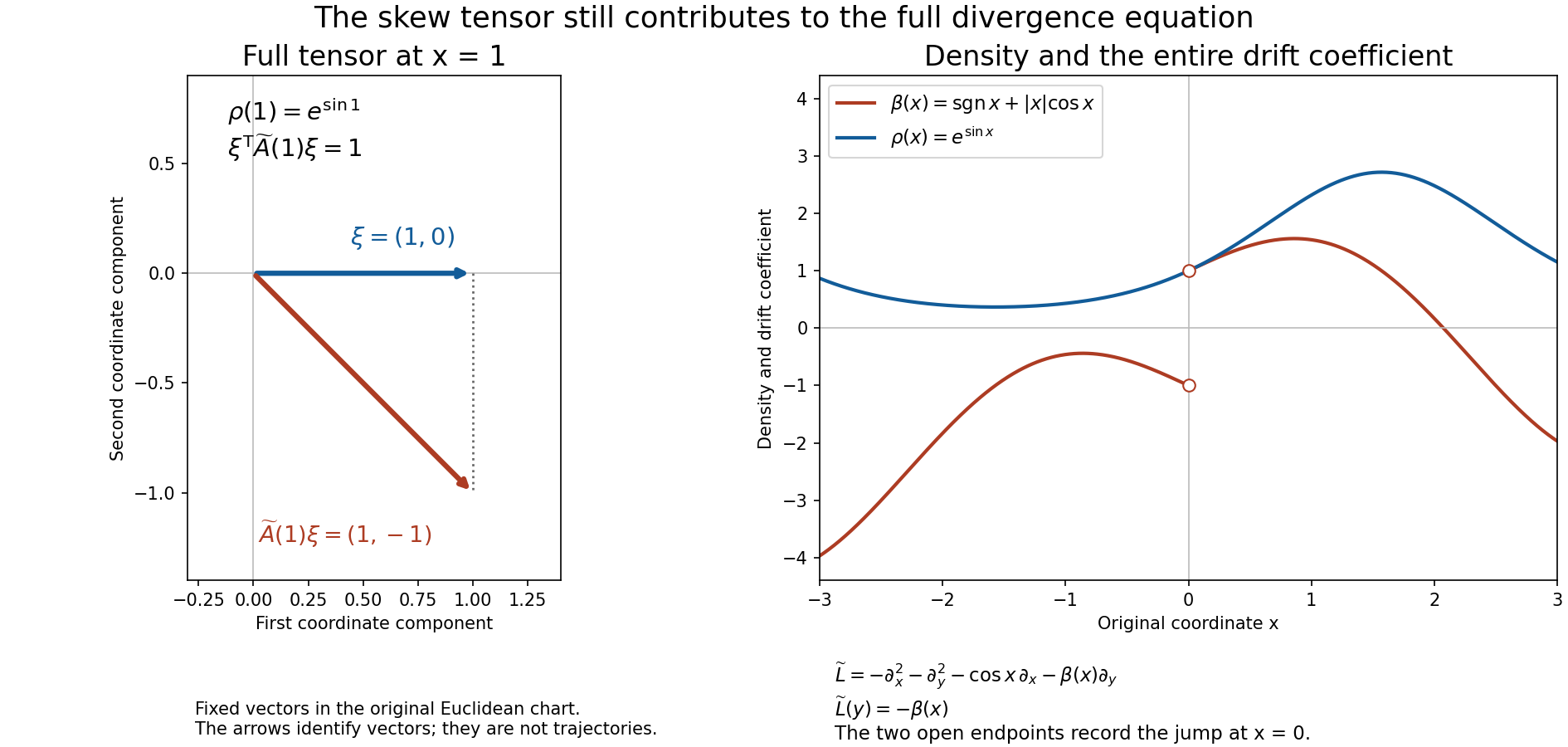
The fixed vectors on the left use the exact original tensor at the indicated coordinate. The curves on the right show the original density and the entire drift in DA16–DA17. The sign function has two open one-sided endpoints at zero; its chosen point value does not affect the weak equation. This is a coordinate diagram, not a trajectory or a physical model.
6. A bounded comparison with the original-author regularity source
The source here is Sergey E. Mikhailov’s original arXiv:0906.3875v3
archive, revised November 21, 2012, and its Part II file
Mik-JCE6-HeC4input.tex. The archive contains the updated
author sources of two published articles. The whole Part II prefix
through line729, including the complete proof of its theorem labeled
RegTh at lines464–725, was read for this comparison. The
later Part II body and the main Part I body are not claimed as read. The
exact freely accessible author version is arXiv:0906.3875v3.
The exact receiving operator and coefficient
classes. The source’s equation 2.1-H,
lines242–247, is
.
Use it here with the full operator
,
coefficient
,
lower coefficients
,
and right side
.
This is equality of the original equations, not replacement of the
density-bearing operator. Its scalar Petrovsky ellipticity follows from
.
The source’s actual adjoint coefficient
,
lines253–256, agrees with DA2 after multiplication by
.
In definition DC^sigma, lines261–266, the full
coefficient conditions are
At an integer exponent the source uses
the corresponding bounded derivative class; at a noninteger exponent its
plus class takes the union of strictly higher exponents. Its theorem
RegTh uses the intersection of coefficient classes at
and
for the direct equation. For
these are
;
for
they are
.
In both cases the leading coefficient need only satisfy the exponent-one
bounded weak-derivative requirement, and
does so locally. All first-order and zeroth-order conditions are
satisfied by their exact zero values. Multiplication by
is bounded on the relevant local
and
spaces. The two source conclusions are therefore precisely the
-to-
and
-to-
receiving assertions. This check does not apply an exponent-one
condition to the expanded density drift in DA9, which can be only
continuous or bounded; using the unexpanded full flux is essential.
Visible Fourier pairing erratum. The source fixes the transform with phase , with inverse phase , at lines151–152. Its scalar bilinear pairing at line140 uses an inverse transform in its first factor. The vector display at line156 instead integrates two forward transforms at the same frequency. With the stated bilinear pairing its correction is For Schwartz functions insert the full inverse formula for the second factor into the left side. Absolute Fubini is justified by ; the first integral is exactly the forward transform of at . For dual Bessel Sobolev classes, weighted Cauchy–Schwarz bounds the right side by their two norms, because . Schwartz density then extends the identity. Thus the frequency reversal is required; it is not a convention-dependent extra power of .
For an explicit counterexample take dimension and vector rank one and , with real . Its transform is . To verify the Gaussian factor directly, the integral of equals one by squaring and polar integration; differentiation of its transform and integration by parts give , . Translation then gives the displayed phase. Hence The second identity follows by scaling the same Gaussian transform and evaluating it at frequency . These values differ. The archived author source remains unchanged; DA19 is a separately identified conceptual erratum.
The course uses the original transform phase and inverse multiplier . Its exact comparison with the source convention is The latter is the full weak-derivative norm . Consequently ; taking dual unit balls gives . The source inner product is linear in its second entry, while the course pairing is linear in its first: their value for the same two arguments is related by complex conjugation. Both conventions and every original transform factor have now been compared explicitly.
The finite-norm justification in the source proof.
In step(i) of RegTh, lines591–619, the displayed estimate
contains the desired
norm of a cutoff of the original unknown. The argument makes its
coefficient positive and concludes that the norm is finite. The
displayed calculation does not first supply a regularization or an
inverse argument proving that this highest norm is finite, so absorption
of that quantity alone leaves a proof gap at that step. This identifies
a missing justification in the read proof, not a counterexample to its
theorem or a claim to have audited all its more general systems and
Holder cases. For the scalar Lipschitz receiving case actually used
here, DA6–DA8 prove the first gain using finite smooth norms and a weak
limit; DA9 and the complete L40–L43 proof establish the second gain
using smooth differences and Cauchy highest derivatives. These supply
the missing finite-norm justification in this course’s exact scope. No
broader source theorem is being silently substituted for the local
proof.
References
The local commutator and elliptic estimates used here are proved in Local inverses and distance-weighted elliptic estimates; the continuation input is in Curved weights and the directions in which support can end. The compact-component qualification above is part of the statement that should be retained whenever the manifold clause is used.
For a direct regularity comparison, Mikhailov, “Solution regularity and co-normal derivatives for elliptic systems with non-smooth coefficients on Lipschitz domains” (2013), Theorem 4.3 of the author postprint, treats a broader system setting and Sobolev indices. Its statement includes the scalar endpoints relevant here. Hunter’s Notes on Partial Differential Equations, revision 18 June 2014, Theorem 4.27, gives a detailed difference-quotient route for real coefficients and an initially weak solution. Those initial conditions differ from our first regularity step.
Malgrange, “Existence et approximation des solutions des équations aux dérivées partielles et des équations de convolution” (1956), Chapter III, relates adjoint continuation, compact hulls and global solvability on a smooth noncompact manifold. Its hull lemma and Theorem III.5 are useful comparisons for the global mechanism. The present argument supplies its own compact-hull construction and weighted estimate in the stated /Lipschitz setting.
Further questions
Three research routes follow from the distinctions established here. First, prescribe a growth class for the data and seek a weight with a quantitative growth bound; the arbitrary locally finite construction does not supply one. Second, add lower-order terms and determine the full adjoint kernel on compact components; constants need no longer describe it. Third, compare interior surjectivity with a chosen boundary condition, where traces and complementing conditions introduce additional constraints. Each question needs its own hypotheses and proof.