Reproduce the compact Fourier division diagrams
Read the full learner and complete formal proof. Every proof, all three worked examples and six complete solutions remain in that reader. Jump to the complete formal proof.
Exact original files
The following original files are supplied without any byte change. The proof download is the entire original CF042 manuscript, including CF1–CF31, all nine sections, examples, solutions, captions and human-source credits.
- compact-fourier-division-proof.md — 29808 bytes; SHA256
917DAFE122DCAED17C08C07DFE795CD3B54B64083BD6617254534AAEA0BBACCB. - make_figures.py — 6775 bytes; SHA256
E6CCA0A8AF4EBC8BAA02316B602572ABE3E7B5F853825E11B6E91593BB8ADFB7. - README-reproduce.md — 975 bytes; SHA256
89912DBCE320DE45CA85F072829ABDFD7E1DB1FB69AADA421DFF97CD3DC763A2. - geometry.json — 1514 bytes; SHA256
E059CED5DBCFD0B82A670D77F33C8758797058E51A0A5870E3217C76BBBEBE91. - support-plane-decay.png — 77877 bytes; SHA256
DE80AEE0D866B22928A13E21F850BCE353390B6290CCA92A871A887A45511D19. - support-plane-decay.svg — 66569 bytes; SHA256
BB72ADC0C6C1CDB54D212251B841965A417F6C3B47398727640E2D322BE12DBA. - safe-division-circle.png — 93101 bytes; SHA256
213E9E794D6CB9541563527F7D4F5252BCF848A6D968404D88B705B38C645673. - safe-division-circle.svg — 60698 bytes; SHA256
33DDC878CE17E88C905A15C69C1E660F143939B71CA727CD8676D0CD5861073B. - double-root-moments.png — 61766 bytes; SHA256
E5E91661169E54574FA80D28104F44BCC118DB5AFDDA9E7028B1916914297463. - double-root-moments.svg — 44468 bytes; SHA256
ED6FDEE37252C08413EC0B769110ABD359273F51FCE539569E477DC307A9888A.
Fresh portable replay
Download the renderer into an empty scratch directory. The original proof and README stay beside it; PNG, SVG and geometry files live in figures/. The renderer requires Python, NumPy and Matplotlib and creates its output directory. Use an explicit fresh output path:
python -B -X utf8 make_figures.py --output-dir fresh-figures
Compare fresh-figures/geometry.json with the supplied exact coordinate ledger, and compare its three PNG and three SVG files with the originals. Do not choose a directory holding the supplied originals. A fresh replay with Python 3.13.9, NumPy 2.4.4, Matplotlib 3.10.9 and Pillow 12.2.0 reproduced all seven output files byte for byte, including the geometry file; all three PNGs also matched in every RGBA channel. Different software or fonts may change rendering bytes even when the geometry is unchanged.
Read the geometry with the proof
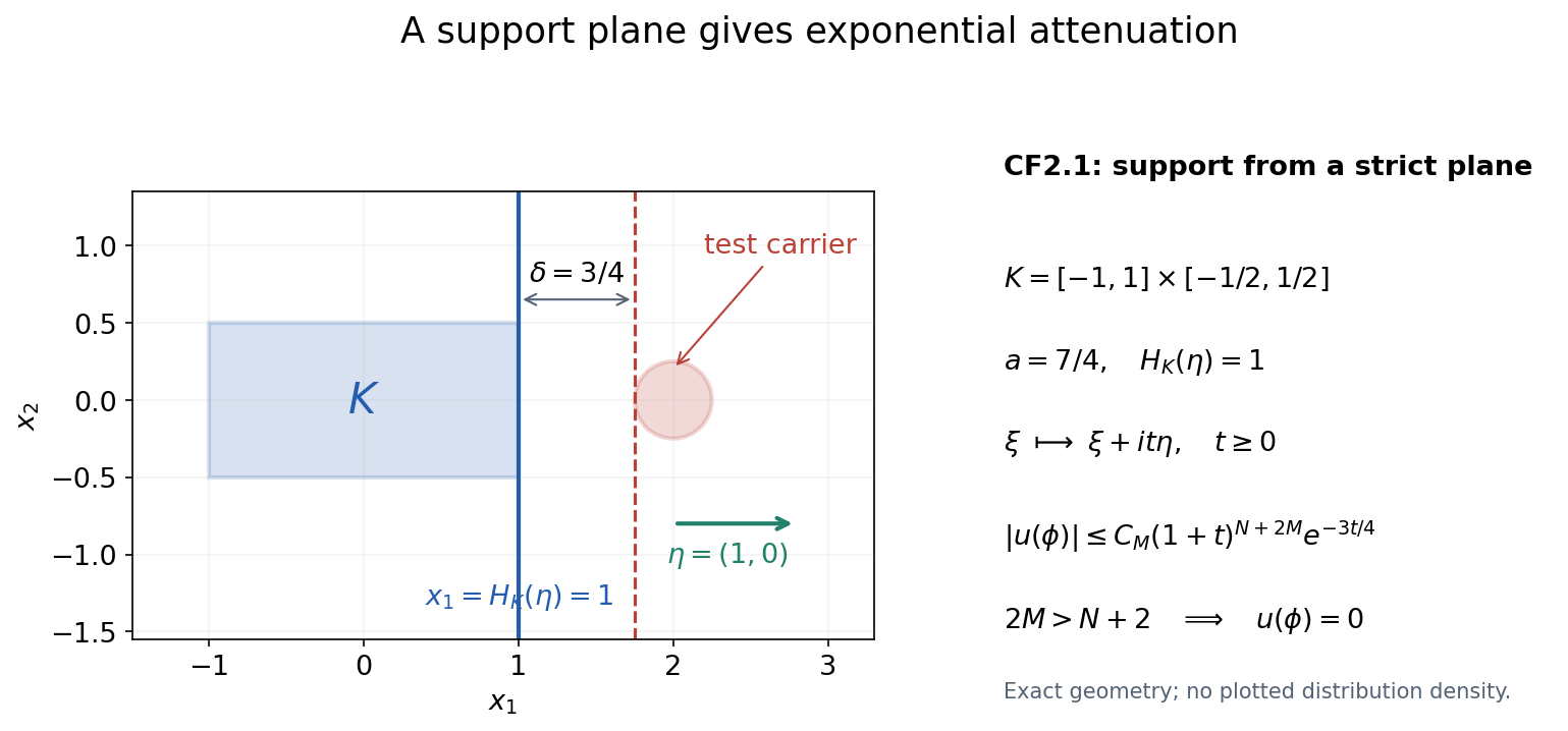
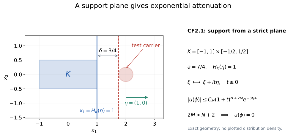
Figure CF-A uses the rectangle K = [−1,1] × [−1/2,1/2], the test disk with center (2,0) and radius 1/4, the unit direction (1,0), supporting planes at 1 and 7/4, and the strict gap 3/4. CF9–CF13 prove the polynomial factor times exp(−3t/4); the drawing is a carrier illustration, not a distribution density.
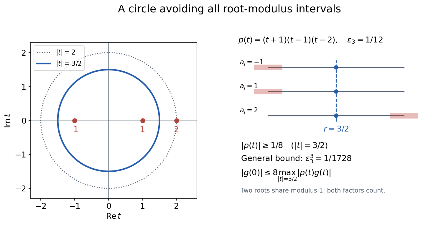
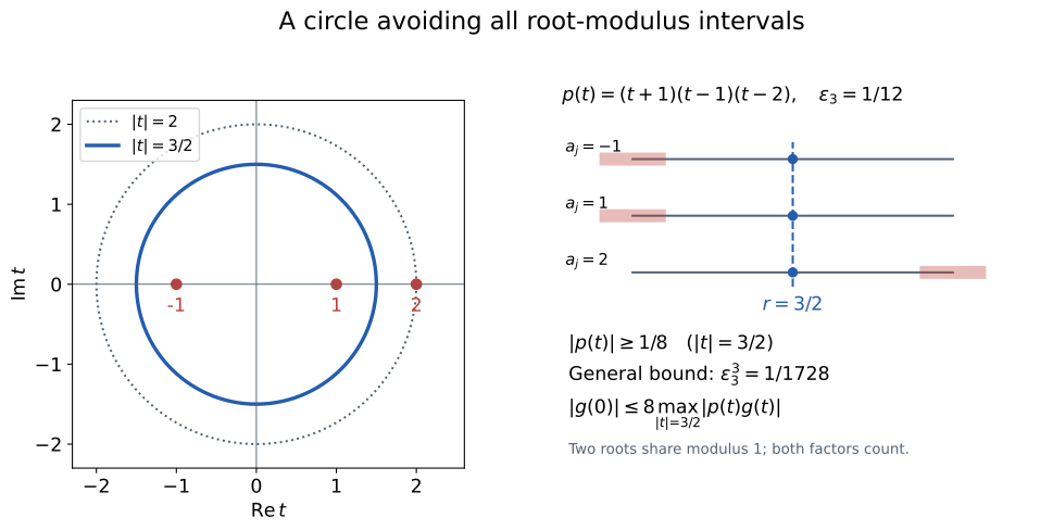
Figure CF-B has p(t) = (t+1)(t−1)(t−2), root-counted degree three, epsilon 1/12, the safe circle of radius 3/2 and the outer disk of radius two. The two roots of modulus one occupy separate interval rows. The bound 1/8 and reciprocal constant eight apply to this example; 1/1728 is the separate universal lower bound. CF14–CF19 and CF29 prove the estimates.
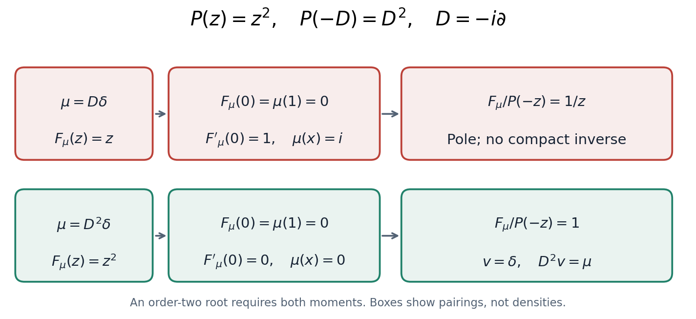
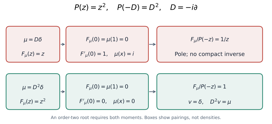
Figure CF-C compares D-delta and its second derivative for P(z) = z². Under D = −i partial, the first derivative has transform z and linear moment i, so its quotient 1/z has a pole. The second derivative has transform z², both required moments vanish, and its compact transpose inverse is delta. CF22–CF28 and the complete caption retain every sign.
Credits and component terms
Credits and CC0 notice retain the original AI author and the human mathematical source. Hörmander, The Analysis of Linear Partial Differential Operators I, second edition, 2003 reprint of the 1990 edition, is the original mathematical source: Theorem 7.3.1; Theorem7.3.2 and Lemma7.3.3; Definition7.3.5 and Lemma7.3.7. The full proof retains those approved locators and its publisher link. Source credit does not transfer the book copyright to CC0. Matplotlib, DejaVu and MathJax keep the component terms already supplied in the course.
The accepted formal module is bounded to the declared Fourier/Cauchy entries, L010 entry(3) and an additional ordinary-hull proof of entry(2), and the L011 entire-annihilator/compact-division statements. The complete Green reader and its earlier alternative are now supplied at their declared entries; the finite rectangle calculation remains given in the learner.