Reproduce the Logarithmic Fourier graphs construct a cone-supported inverse
These original drawings accompany Logarithmic Fourier graphs construct a cone-supported inverse. The complete mathematical proof, all worked examples and complete solutions remain in that reader.
Download the unchanged original files
Keep make_figures.py at the root of an empty scratch directory and the PNG, SVG and geometry files in figures/. The three unchanged Markdown sources and CREDITS.txt/LICENSE.txt stay at the package root; they are downloads and are not generated by the renderer. The renderer creates figures/ during a fresh run.
- make_figures.py — 12768 bytes; SHA-256
74DE844A388E1E72C454C1DADEF38DB26848F721B3563A6958777C6059861188. - geometry.json — 2855 bytes; SHA-256
7BE6AD84A74863F83E26D6C9D0075360D6B104C80767CE0AB15A8D370906D766. - logarithmic-cutoff-and-jacobian.png — 198251 bytes; SHA-256
108980A9AEE95641A978ED1337F703E10AC90EC669E00CC24A556330C636CE6C. - logarithmic-cutoff-and-jacobian.svg — 106660 bytes; SHA-256
C26D639A33242E16A54D4A5CDAE2414BE37EA0933F0444EF3862E3C356DEABA5. - support-plane-and-uniform-decay.png — 209810 bytes; SHA-256
B4C6D1145F69192F6D9EB33C8F1387225E96FC49F25B6F6E94213C24A34FF478. - support-plane-and-uniform-decay.svg — 104160 bytes; SHA-256
721E02447A86F6CE6C6E3AEFF6F136E2A916D3304F13B43D37C6E3907A4F0A0E. - two-variable-graph-and-directions.png — 340326 bytes; SHA-256
57A21A7399984F839DA726AB79469BA7878892C9DB00114F63001B2AFABB5FC0. - two-variable-graph-and-directions.svg — 888813 bytes; SHA-256
22B143DC261176B4B89083D21E8E1863F59826B8A5B375FE54B9C69595C02A13. - learner-full.md — 52320 bytes; SHA-256
14B84E4377A395E0FB24A72C170D6FB4279DBD855C456C5A9670082849551DF1. - manuscript.md — 38116 bytes; SHA-256
B16110319C93285E2ABF2A348CAEBD22E02FBA6C501189C1B2FB2140EF40E018. - learner.md — 14658 bytes; SHA-256
BC7793430A395A74C3D1E382F30B743F5FBBFDF832F7FFEBE5FC0632FA3D3F6E. - LICENSE.txt — 522 bytes; SHA-256
25E18118514AA1C4E2716F8F88557709A630213080B33E37BFCAEB1A9BA3702A. - CREDITS.txt — 2145 bytes; SHA-256
FE1DC532A41DAB0DC0659E848A42D8B80D8A52E6B129B17B099A8459E8E4C001.
Run the renderer
The unchanged program requires Python, NumPy and Matplotlib. In the scratch directory run:
python -X utf8 make_figures.py
It writes the supplied PNG, SVG and exact geometry files. A fresh replay with Python 3.13.9, NumPy 2.4.4 and Matplotlib 3.10.9, using Matplotlib’s bundled DejaVu Sans font, matched the eight renderer/figure files byte for byte and all three decoded PNG RGBA pixel arrays. No SVG date or identifier normalization was performed. Byte identity is qualified by that observed software and font environment; different versions may change rendering bytes. The geometry files specify the mathematical objects independently of rendering.
Check the mathematics and credits
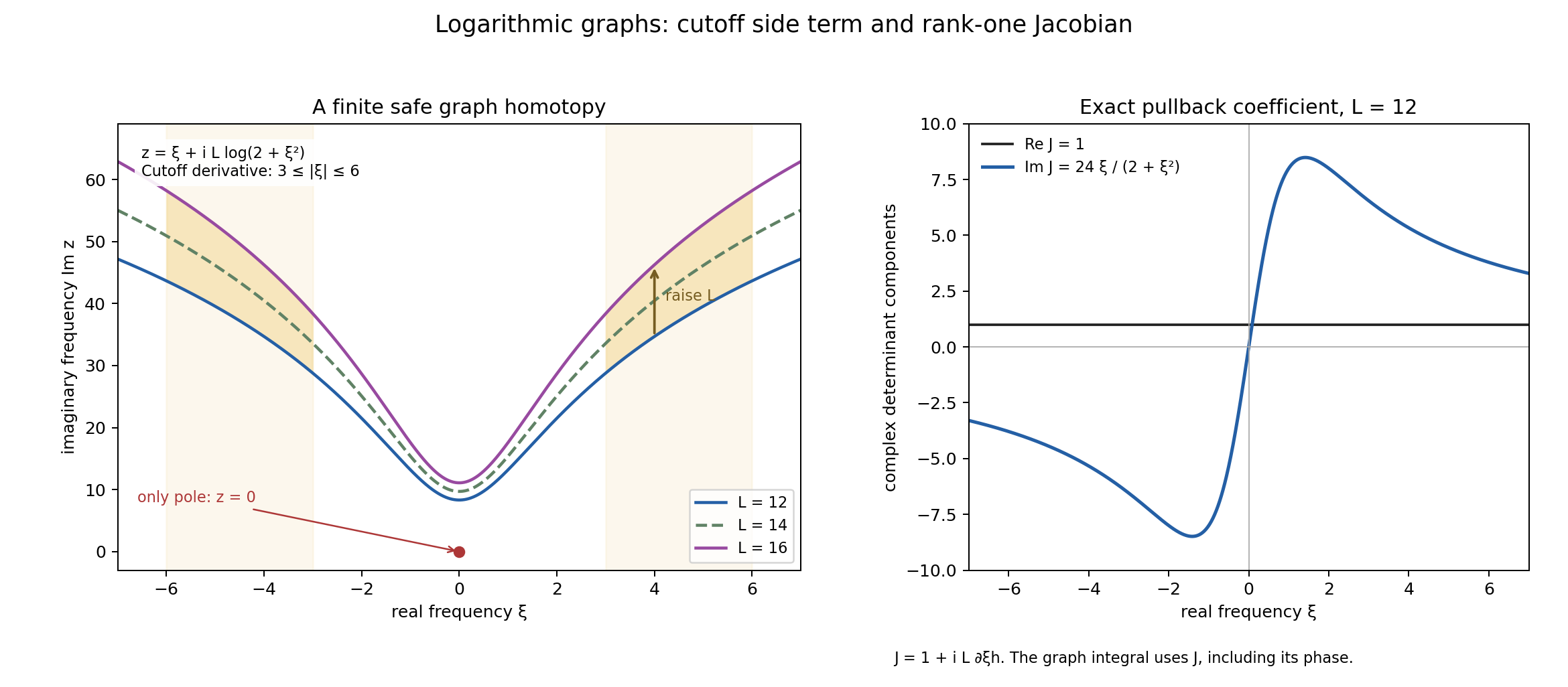
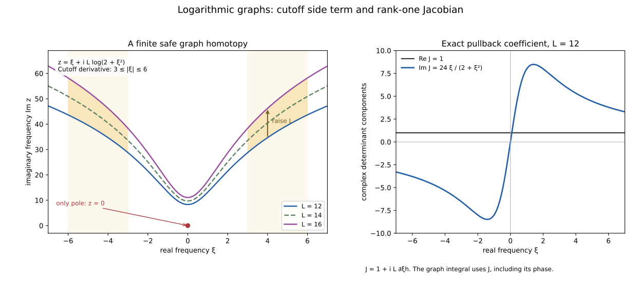
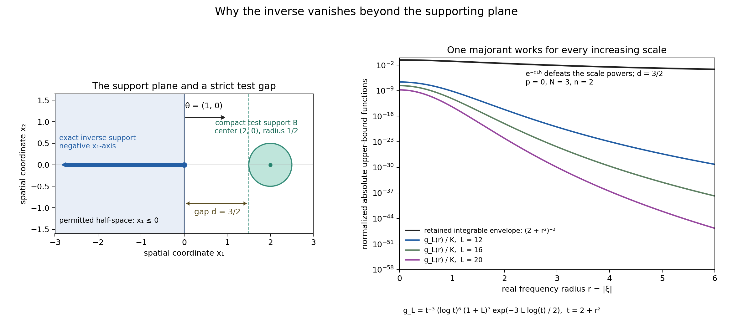
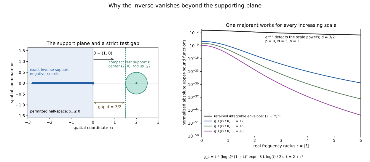
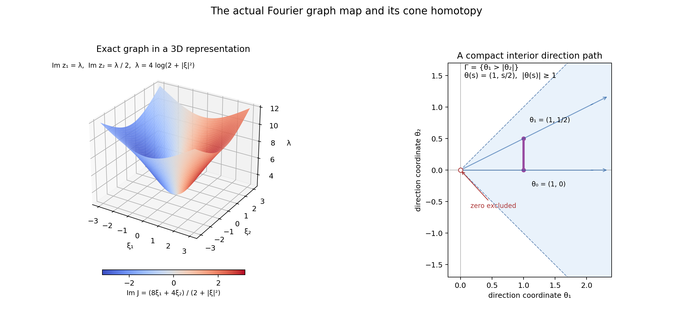
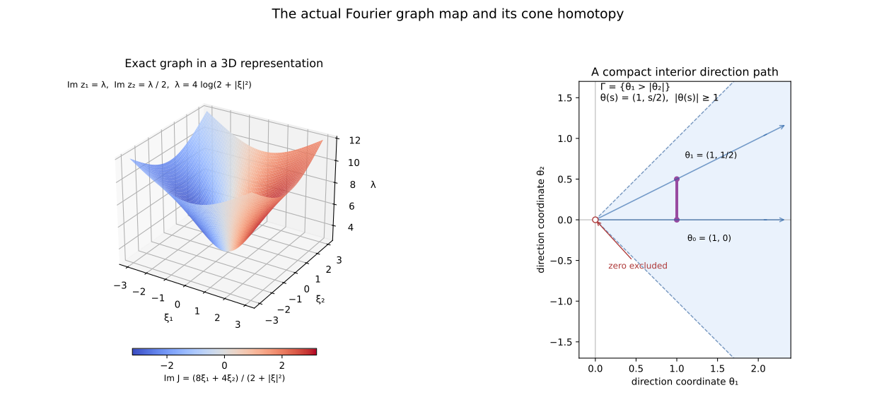
Figure 1 uses the exact graph z = ξ + i L log(2 + ξ²), L = 12, 14, 16, the only pole at zero, cutoff R = 3 and derivative region 3 ≤ |ξ| ≤ 6, and exact complex Jacobian J = 1 + 24iξ/(2 + ξ²) at L = 12. Figure 2 uses z = (ξ₁ + 4ih, ξ₂ + 2ih), h = log(2 + |ξ|²), λ = 4h and exactly recoverable Im z₂ = λ/2; color gives Im J. The path θ(s) = (1,s/2) lies in θ₁ > |θ₂|; it does not certify a kernel threshold at L = 4. Figure 3 uses the exact inverse −H(−x₁) ⊗ δ₀(x₂), its negative-axis support, θ = (1,0), A = p = 0, disk center (2,0), radius 1/2, gap d = 3/2, n = 2 and N = 3. Its curves are proved upper-bound functions with one integrable envelope, not measurements. Full captions, equations (5.8)–(5.11), (8.3)–(8.7), and Problems 2, 6 and 9 give the precise proof locators.
The exact original complete source, formal proof and exercise source are retained above. The theorem produces one common inverse for a nonempty ordinarily convex open positive-dilation cone excluding zero under uniform closed-angular logarithmic reciprocal bounds. Semyon Dyatlov, Gerd Grubb and Lars Hörmander receive the full comparison credits above and in CREDITS.txt; external copyrighted prose and media are absent. See the complete included convolution reading, Theorem 1.1, equations (1.4)–(1.8).
The original renderer, scene/geometry and diagrams are GPT-6.1 Sol (OpenAI), Ultra work, October 2026, dedicated under CC0. Matplotlib and the bundled DejaVu Sans font retain their own component terms already included with this course. The native geometry is explanatory; the full proof establishes the theorem.