Reproduce the L112 null-section figures
The two original figures in Null-section curvature and the Riesz comparison show the Lorentz null frame, the Gaussian/ambient mean-curvature identity, and finite or absent reflected focal values. The proof uses three spatial dimensions, \(G=c^2dt^2-|dx|^2\), the positive induced surface metric \(g=-G\), and the squared-separation-normalized reflected vector \(\nu=-L/2\).
Download and run
Download build_and_check.py into an empty folder. No additional file is needed. From that folder, with Python 3.13, run:
python -m pip install numpy==2.4.4 sympy==1.13.1 scipy==1.17.1 matplotlib==3.10.9
python build_and_check.py
The script creates a figures subfolder and writes both PNGs, both SVGs and both geometry JSONs listed below. It also runs 15 exact symbolic checks of arbitrary radial two-jets and 24 polynomial wave-integral checks. Its locally generated computational-checks.json is a diagnostic record, not part of the downloadable reproduction package.
The observed reproduction environment was Python 3.13.9, NumPy 2.4.4, SymPy 1.13.1, SciPy 1.17.1 and Matplotlib 3.10.9, with DejaVu Sans and the Agg renderer. Pillow 12.2.0 was used only for the package's image inspection. The script uses no TeX or Blender.
Figure 1 and its exact geometry
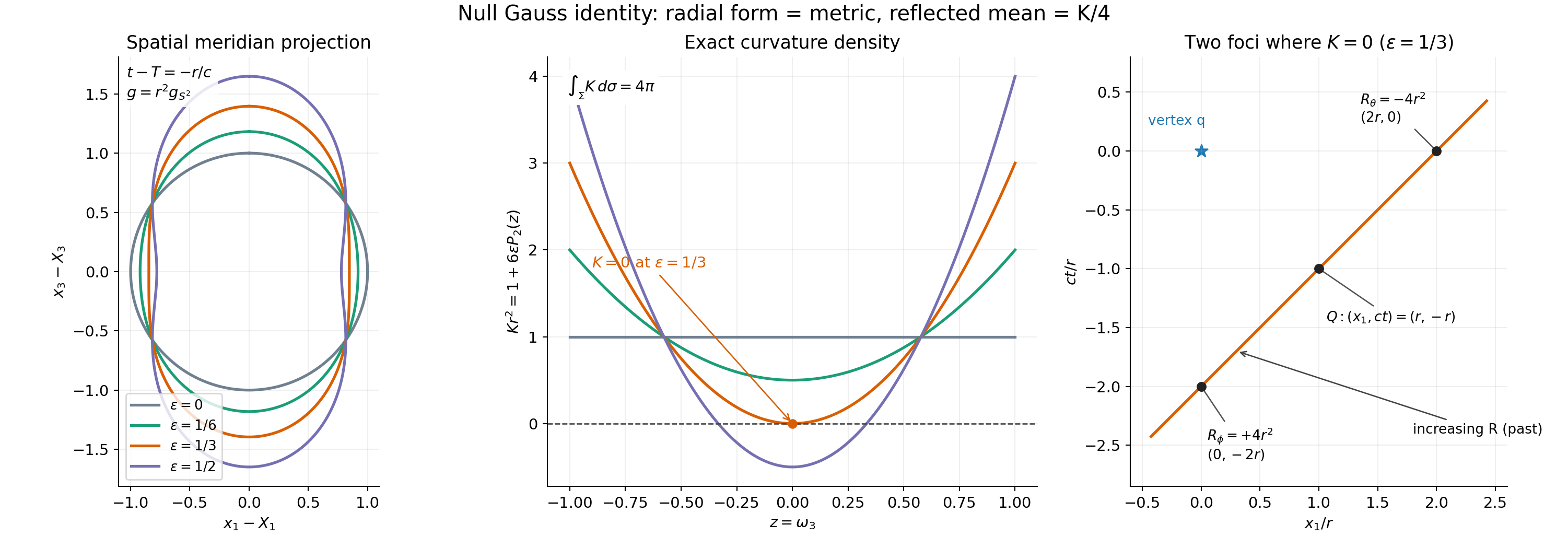
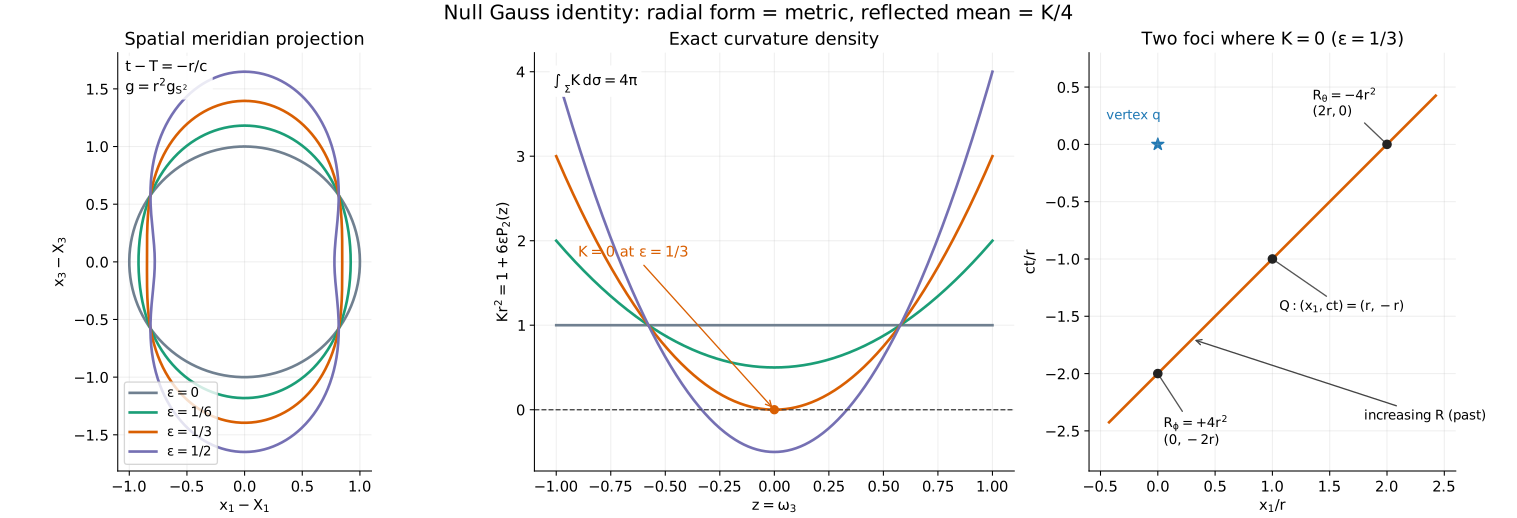
The spatial meridian is the projection of \(r=\exp(\epsilon P_2(\omega_3))\), \(P_2(z)=(3z^2-1)/2\), with \(t-T=-r/c\). It is not the induced surface metric. The middle panel plots exactly \(Kr^2=1+6\epsilon P_2(z)\). At the equator with \(\epsilon=1/3\), the reflected line has focal parameters \(-4r^2\) and \(+4r^2\); the negative value lies on the future continuation and the positive value on the past reflected ray. See the lesson's equations (11), (16), (23) and its complete Figure 1 caption. The original Riesz focal interpretation is located in the lesson's free primary reference [R49], section 68, pages 138–141.
Figure 2 and the degenerate cases
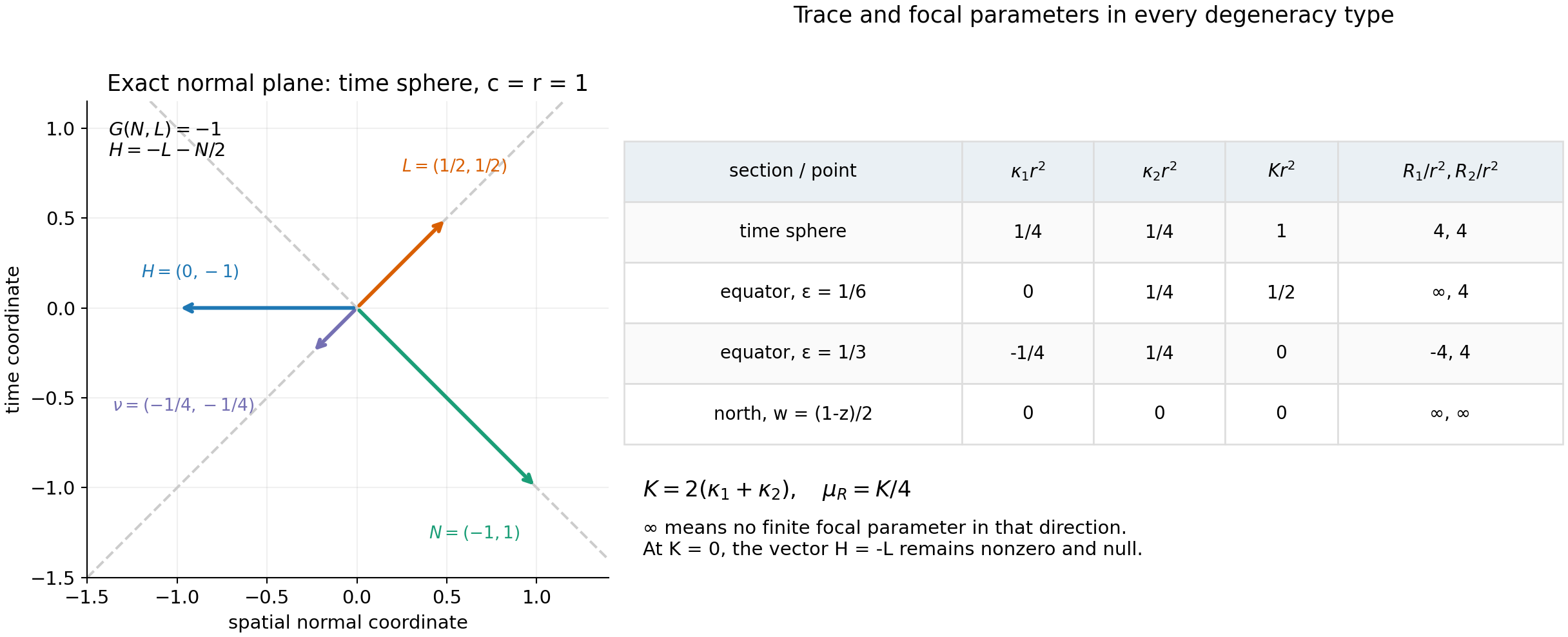
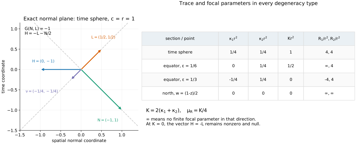
The normal-plane panel takes \(c=r=1\) and lists vectors as (time, spatial normal coordinate). Its exact vectors are \(N=(-1,1)\), \(L=(1/2,1/2)\), \(\nu=(-1/4,-1/4)\) and \(H=(0,-1)\). The table includes repeated nonzero, one zero, cancelling nonzero and two zero reflected-shape eigenvalues. Infinity denotes no finite focal parameter. See Theorem 2, equations (13)–(17), the examples and Exercise 6; the full caption retains these qualifications.
What can be compared exactly?
The copied script and six supplied outputs are bound to the accepted corrected source. The package's isolated replay compares both PNGs and both geometry JSON files byte for byte in the observed environment. Font libraries or renderer versions on another machine can change image bytes even when the coordinates are unchanged; the geometry JSONs and proof locators identify what to check mathematically.
Raw SVG byte equality is not promised. Matplotlib includes a creation timestamp and generated element IDs. The replay comparison removes the timestamp and consistently renames IDs and their references before comparing normalized SVG content. These changes do not alter paths, text, transforms or coordinates. Keep the downloaded originals for exact archival hashes.
The course remains a draft.