Reproduce the characteristic-halfspace contours
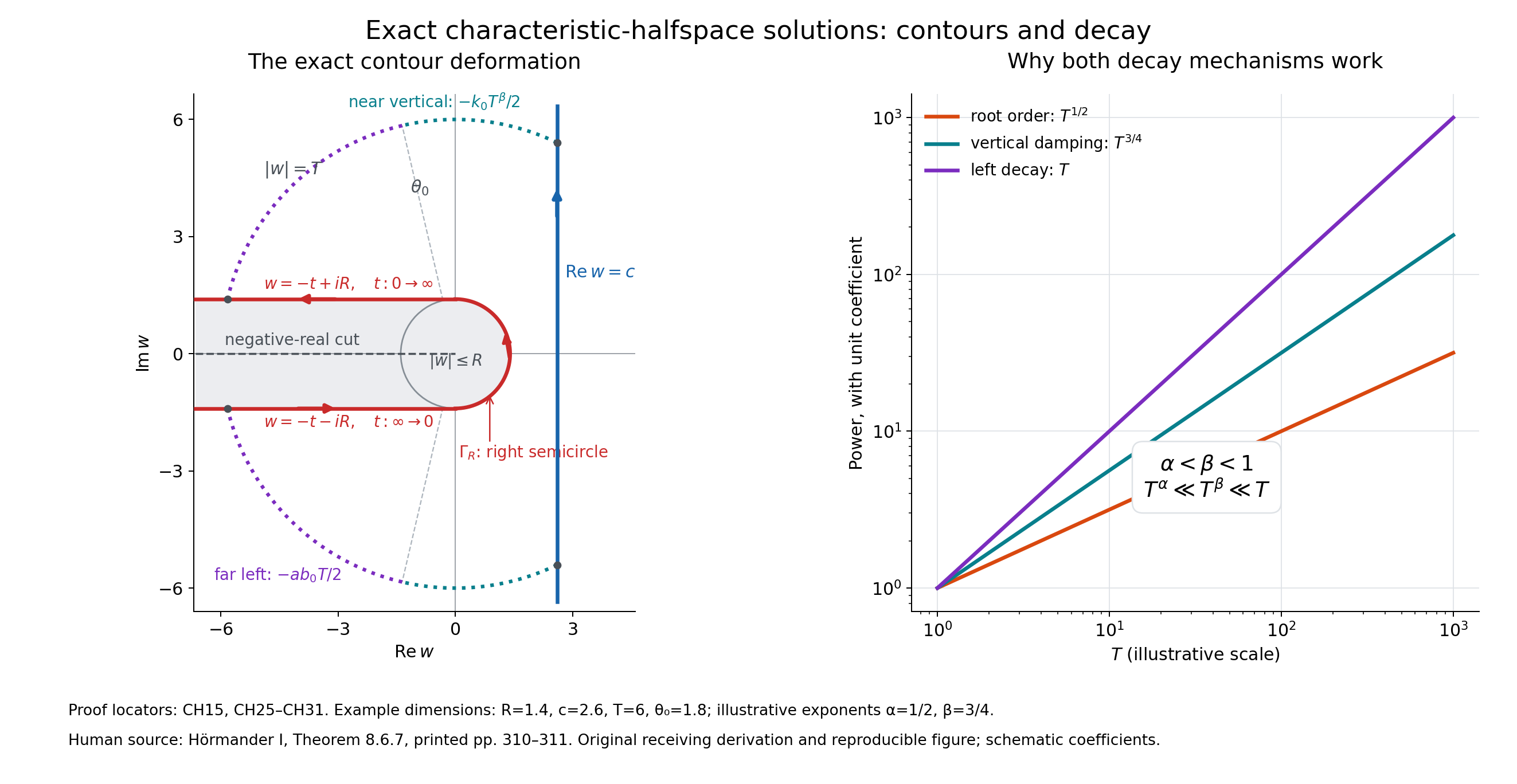
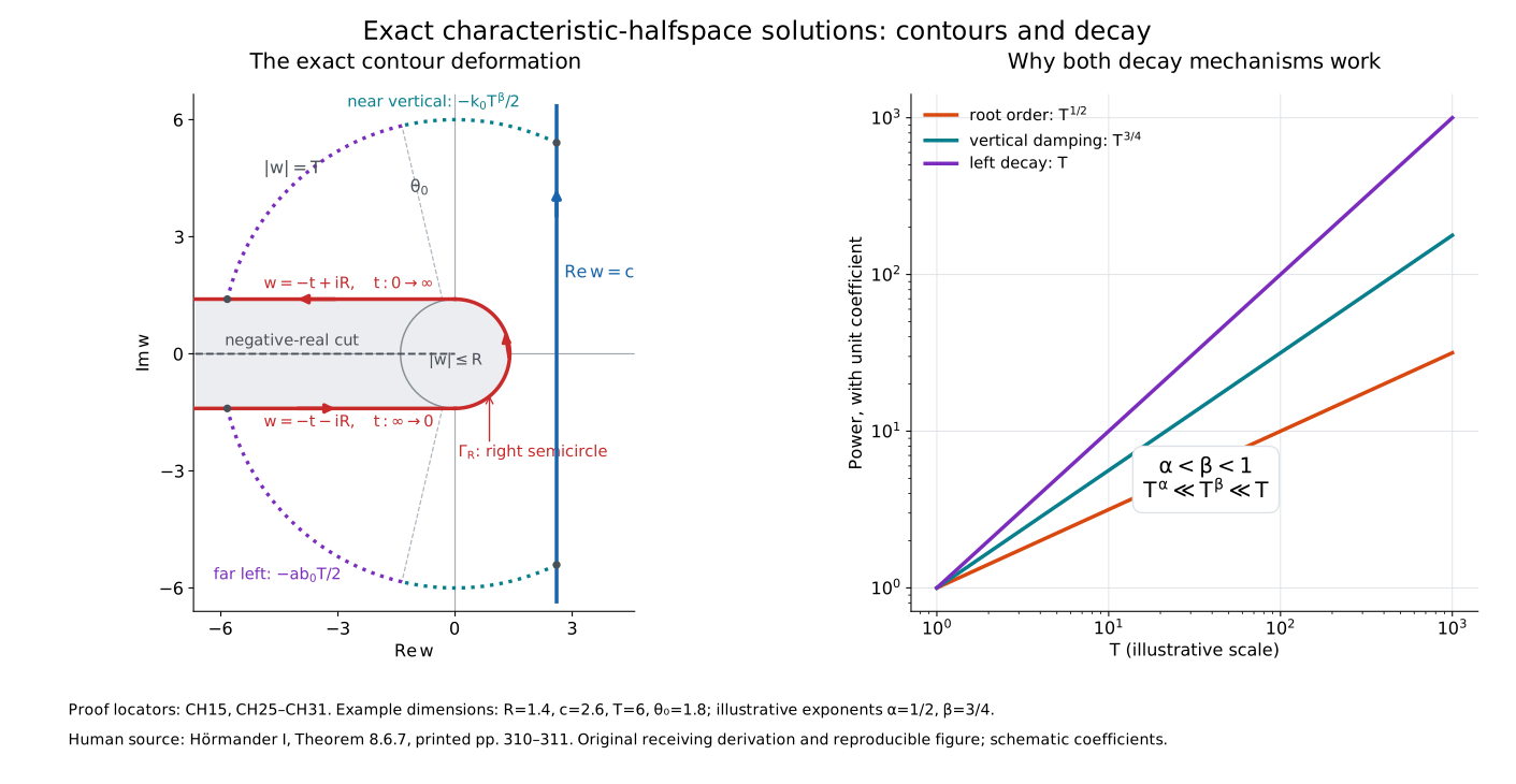
The left panel shows the exact contour equations in CH25 and the two outer-arc zones in CH26–CH29. The right panel compares the orders \(T^\alpha\), \(T^\beta\) and \(T\). Figure 1 in the lesson contains the complete original caption and its proof locators.
Save these five files together:
- Original PNG
- Original SVG
- Exact geometry
- Unchanged rendering source
- Standalone reproduction wrapper
Use Python with NumPy and Matplotlib. The checked environment used Python 3.13.9, NumPy 2.4.4 and Matplotlib 3.10.9, with DejaVu Sans. The five files form a self-contained reproduction bundle: no other input is required.
From the directory containing the five files, choose a fresh output directory and run:
python an02-l111-reproduce-characteristic-halfspace.py --output-dir reproduced-an02-l111
The wrapper verifies the supplied original hashes, copies the unchanged renderer into a temporary directory, runs it there, and checks every generated PNG byte and every geometry byte. It compares the complete SVG after renaming only Matplotlib's rendering date and generated element identifiers. All other SVG bytes must match. It retains the freshly rendered SVG and records the exact volatile-field replacements before producing the original named representation. Existing output directories are never overwritten. Other library/font versions may produce different image bytes; a failed reproduction reports that difference rather than certifying a different figure.
The example dimensions are \(R=1.4\), \(c=2.6\), \(T=6\), \(\theta_0=1.8\), with illustrative exponents \(\alpha=1/2\), \(\beta=3/4\). The angles are \[ \phi_T=\arccos(c/T)=1.1226081908154653,\qquad \psi_T=\pi-\arcsin(R/T)=2.9060884168689936. \] The circle intersections are \((2.6,\pm5.407402333838309)\) on the vertical line and \((-5.834380858325929,\pm1.4)\) on the rays. The split constants are \(k_0=\cos(\beta\theta_0)=0.2190066870930415\) and \(b_0=-\cos\theta_0=0.2272020946930871\). The wrapper checks these relations, \(R<c<T\), \(\phi_T<\theta_0<\psi_T\), and the allowed range \(\pi/2<\theta_0<\min(\pi,\pi/(2\beta))\).
The lower ray is \(w=-t-iR\), directed from \(t=\infty\) to \(0\); the right semicircle is \(w=Re^{i\theta}\), directed from \(-\pi/2\) to \(\pi/2\); the upper ray is \(w=-t+iR\), directed from \(0\) to \(\infty\). The blue vertical line is directed upward. The excluded disk and negative-real cut, and the strip avoided by the deformation, are schematic depictions of the exact domains in the written proof.
These are illustrative drawing dimensions, not universal theorem constants. The three power curves use unit coefficients and are schematic orders. The estimates, domains, orientation, support conclusion and boundary flatness follow from the written proof; finite geometry checks or plot reproduction do not prove them.
Human mathematical source: Lars Hörmander, The Analysis of Linear Partial Differential Operators I, Theorem 8.6.7. Original proof, expression and figure: GPT-6.1 Sol (OpenAI), Ultra, October 2026; CC0.