Reproduce the arbitrary-order perturbation figure
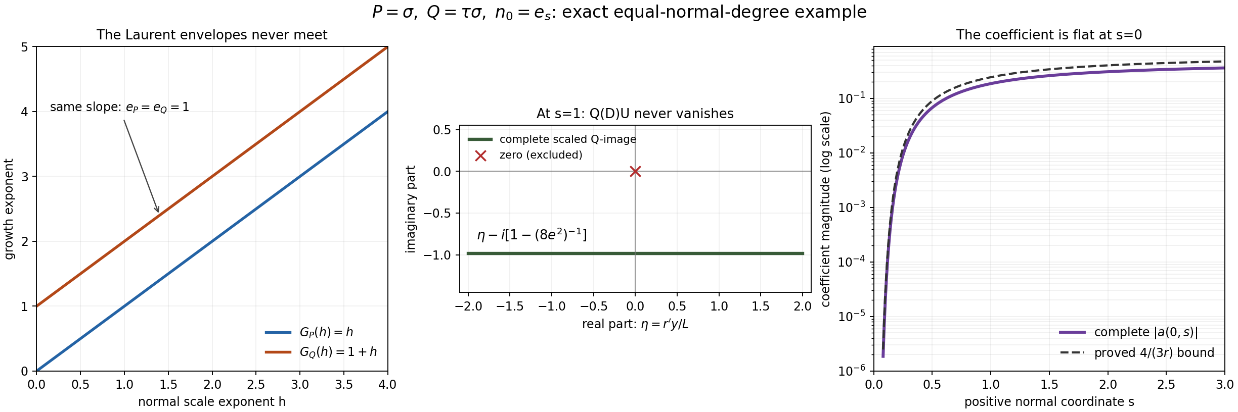
The three panels show the exact pair \(P=\sigma\), \(Q=\tau\sigma\), \(n_0=e_s\), with \(R=2\) and \(A=2\). The left panel compares the growth envelopes; the middle panel shows the complete scaled Q-image at \(s=1\); the right panel shows the complete coefficient modulus on \(y=0\) and its proved upper bound. Figure 1 in the lesson gives the exact formulas and interpretation.
Save all five files together:
- Original PNG
- Original SVG
- Exact geometry and historical inspection metadata
- Unchanged renderer and 206 bounded algebra/model checks
- Standalone reproduction wrapper
Use Python with NumPy, SymPy and Matplotlib. The checked reproduction used Python 3.13.9, NumPy 2.4.4, SymPy 1.13.1 and Matplotlib 3.10.9. Different rendering-library versions or fonts may change picture bytes; the wrapper fails clearly if the mathematical figure no longer matches its supplied original. No other input is required.
From the directory containing the five files, choose an output directory that does not exist and run:
python an02-l110-reproduce-higher-order-q.py --output-dir reproduced-an02-l110
The wrapper copies the unchanged rendering source to a temporary directory, executes all 206 checks, renders all three panels, and verifies the whole figure and geometry before creating the named outputs. It leaves the supplied originals untouched.
The PNG must reproduce exactly. Matplotlib's SVG includes a rendering date and generated element identifiers; the wrapper compares the complete SVG after renaming only those volatile fields, then restores their original representation. It records every such replacement and retains the fresh unnormalized SVG. Every other SVG byte must match.
The renderer also regenerates the complete mathematical geometry description. The supplied geometry includes an original historical visual-inspection annotation added after rendering. The wrapper checks all mathematical and descriptive fields, preserves that annotation separately, and records the distinction. It retains the freshly generated unannotated geometry. The final named PNG, SVG and geometry files have exactly the supplied original bytes.
The output directory also contains the complete fresh 206-check report and a reproduction record with versions, verification details and exact file digests. The numerical samples and symbolic checks supplement the lesson's written proof. They do not replace its global denominator estimates, support argument or proof that every boundary derivative vanishes.
The original proof, expressions and figure are GPT-6.1 Sol (OpenAI), Ultra, October 2026; CC0.