Weyl kernels, operator traces, and a finite trace-class test

Written and dedicated to the public domain by Codex, September 2026 (CC0).

A Weyl symbol lives on phase space, while its operator acts on a Hilbert space. To compare their traces, we first identify every Hilbert–Schmidt kernel and its exact Fourier factor. A trace-class operator with an integrable Weyl symbol then has a phase-space trace, even when its kernel has no continuous diagonal. Finally, a finite list of weighted symbol derivatives gives a concrete trace-class test. The integer $n+1$ is forced by the oscillator spectrum in $n$ configuration variables; no index formula is needed for these results.

The needed course lessons are Symbols, operators and Sobolev scales for the Fourier convention $D=-i\partial$, Weyl quantization, Plancherel and symbolic composition, and Traces that survive passage to cohomology for Hilbert–Schmidt operators, trace-class products, polar factorization and matrix traces. We prove the additional kernel, diagonal and weighted-derivative steps here. This lesson concerns the original matrix symbol on $\mathbb R^{2n}_{x,\xi}$; the analytic index integral requires further arguments.

1. Hilbert–Schmidt maps and their complete kernels

Put $H_\nu=L^2(\mathbb R^n;\mathbb C^\nu)$ and $H_\mu=L^2(\mathbb R^n;\mathbb C^\mu)$, with inner products linear in the first variable. A measurable matrix kernel $K(x,y)\in\operatorname{Hom}(\mathbb C^\nu,\mathbb C^\mu)$ is squared with its full Hilbert–Schmidt fiber norm $\operatorname{tr}_{\mathbb C^\nu}(K(x,y)^*K(x,y))$. If $K\in L^2(\mathbb R^{2n})$, Cauchy–Schwarz in $y$ gives $$\|T_Ku\|_{H_\mu}^2 \leq \|K\|_{L^2_{x,y};\mathrm{HS}}^2\,\|u\|_{H_\nu}^2,\qquad T_Ku(x)=\int_{\mathbb R^n}K(x,y)u(y)\,dy . \tag{CI1}$$ The integral exists for almost every $x$. To recover the exact Hilbert–Schmidt norm, take an orthonormal basis $(e_j)$ of $H_\nu$. For almost every $x$, Parseval in the input Hilbert space identifies $\sum_j\|T_Ke_j(x)\|_{\mathbb C^\mu}^2$ with the squared $L^2_y$ norm of the whole matrix row $K(x,\cdot)$. Tonelli then gives $$\|T_K\|_{\mathcal S_2(H_\nu,H_\mu)}^2 =\sum_j\|T_Ke_j\|_{H_\mu}^2 =\iint_{\mathbb R^{2n}} \operatorname{tr}_{\mathbb C^\nu}(K^*K)(x,y)\,dx\,dy. \tag{CI2}$$ Conversely, for an arbitrary Hilbert–Schmidt $T:H_\nu\to H_\mu$, the finite-rank kernel sums $$K_N(x,y)=\sum_{j=1}^N(Te_j)(x)e_j(y)^* \tag{CI3}$$ are Cauchy in the full matrix-valued $L^2_{x,y}$ norm, since orthonormality in $y$ makes the squared norm of a tail equal to $\sum_{j=M+1}^N\|Te_j\|^2$. Let $K$ be their $L^2$ limit. Each $T_{K_N}$ agrees with $T$ on the first $N$ basis vectors, and (CI1) makes $T_{K_N}\to T_K$ in operator norm. Density of the finite basis spans and the Hilbert–Schmidt bound make $T=T_K$. Thus square-integrable kernels and Hilbert–Schmidt maps are isometrically the same objects, with no unmentioned smoothness assumption.

2. The exact Weyl factor

Use the original Fourier convention $D=-i\partial$ and inverse coefficient $(2\pi)^{-n}$. For a matrix Weyl symbol $a(u,\xi)$, its kernel is the partial inverse Fourier transform $$K_{a^w}(x,y) =(2\pi)^{-n}\int_{\mathbb R^n} e^{i(x-y)\cdot\xi}\, a\!\left(\frac{x+y}{2},\xi\right)d\xi . \tag{CI4}$$ This first holds for Schwartz symbols. The linear change $u=(x+y)/2,\ v=x-y$ has absolute Jacobian one: in one coordinate pair its inverse matrix $\left(\begin{smallmatrix}1&1/2\\1&-1/2\end{smallmatrix}\right)$ has determinant $-1$, and the $n$ coordinate pairs multiply the absolute values. Plancherel in $v$, with the exact inverse Fourier coefficient in (CI4), gives $$\|a^w\|_{\mathcal S_2(H_\nu)}^2 =(2\pi)^{-n}\iint_{\mathbb R^{2n}} \operatorname{tr}_{\mathbb C^\nu}(a(u,\xi)^*a(u,\xi)) \,du\,d\xi . \tag{CI5}$$ Schwartz functions are dense in matrix $L^2(\mathbb R^{2n})$, and both sides of (CI5) are complete. The partial Fourier transform in (CI4) therefore extends the identity to every $L^2$ Weyl symbol. Conversely (CI3), followed by the invertible coordinate change and partial Fourier transform, gives a unique $L^2$ Weyl symbol for every Hilbert–Schmidt operator. This also proves that the symbol-to-kernel map is injective at the $L^2$ level.

3. Continuous trace-class kernels and their diagonal

Let $T:H_\nu\to H_\nu$ be trace class. Its polar factorization gives $T=AB$ with $A=U|T|^{1/2}$ and $B=|T|^{1/2}$, both Hilbert–Schmidt; the trace lesson proves the exact norm identity and finite-rank approximation used here. Let their $L^2$ kernels be $A(x,z)$ and $B(z,y)$. Cauchy–Schwarz in $z$ makes $$K_T(x,y)=\int_{\mathbb R^n}A(x,z)B(z,y)\,dz \quad\text{for almost every }(x,y), \tag{CI6}$$ and bounds its absolute matrix norm by $\|A(x,\cdot)\|_{L^2_z}\|B(\cdot,y)\|_{L^2_z}$, an $L^2_{x,y}$ product. Fubini first proves that its operator is $AB$ on compact smooth tests; the $L^2$ bound and density then prove it on all $H_\nu$. In particular this is the unique Hilbert–Schmidt kernel of $T$.

The diagonal factorization $k(x)=\int A(x,z)B(z,x)\,dz$ is defined for almost every $x$. Matrix Cauchy–Schwarz and then scalar Cauchy–Schwarz in $x$ show $k\in L^1_x$. Finite-rank kernel approximation of $A,B$, together with $\|A_1B_1-A_2B_2\|_1 \leq\|A_1-A_2\|_2\|B_1\|_2+\|A_2\|_2\|B_1-B_2\|_2$, gives the exact trace identity $$\operatorname{Tr}T =\int_{\mathbb R^n}\operatorname{tr}_{\mathbb C^\nu} \left(\int_{\mathbb R^n}A(x,z)B(z,x)\,dz\right)dx. \tag{CI7}$$ For finite rank this is a direct sum of rank-one inner products; the displayed trace-norm bound and $L^1$ bound pass the identity to the Hilbert–Schmidt factors.

If the operator kernel has a continuous representative $K_T(x,y)$, its actual diagonal equals $k(x)$ almost everywhere. Here is the step that avoids assigning arbitrary values to an $L^2$ kernel on a measure-zero diagonal. Regard $y\mapsto B(\cdot,y)$ as an $L^2_z$-valued $L^2_y$ function. At almost every $x$, it has an $L^2_z$-valued Lebesgue point $y=x$, while $A(x,\cdot)\in L^2_z$, and (CI6) holds for almost every $y$. Average (CI6) over a ball $B_\varepsilon(x)$ in $y$. The average of $B(\cdot,y)$ tends to $B(\cdot,x)$ in $L^2_z$, so its pairing with $A(x,\cdot)$ tends to $k(x)$. The continuous representative’s average tends to $K_T(x,x)$. Therefore $$\operatorname{Tr}T =\int_{\mathbb R^n}\operatorname{tr}_{\mathbb C^\nu}K_T(x,x)\,dx \quad\text{when }K_T\text{ has a continuous representative.} \tag{CI8}$$ The integral is absolutely defined because the diagonal agrees almost everywhere with the $L^1$ factorization in (CI7). No compactness of $\mathbb R^n$ or positivity of $T$ was used.

4. The trace of an integrable Weyl symbol

The diagonal argument in Section 3 does not automatically apply to a trace-class Weyl operator with merely $a\in L^1$; the kernel need not be continuous. Use a coherent-state resolution that keeps the Weyl coefficient. Let $g(x)=\pi^{-n/4}e^{-|x|^2/2}$, $\|g\|_2=1$, and $g_{q,p}(x)=e^{ip\cdot(x-q/2)}g(x-q)$. Fourier inversion in $p$, followed by $\int|g(x-q)|^2dq=1$, proves for $u,v\in\mathcal S$ and then for all $L^2$ vectors that $$(2\pi)^{-n}\iint_{\mathbb R^{2n}} \langle u,g_{q,p}\rangle \langle g_{q,p},v\rangle\,dq\,dp =\langle u,v\rangle . \tag{CI9}$$ The phases involving $q/2$ cancel in this product. Cauchy–Schwarz and (CI9) give an absolute integral bound $(2\pi)^{-n}\int|\langle w,g_{q,p}\rangle \langle g_{q,p},v\rangle|\,dq\,dp\leq\|w\|_2\|v\|_2$. Expand a trace-class $T$ as a trace-norm convergent sum of rank-one maps with total coefficient sum $\|T\|_1$. The bound permits termwise integration and proves $$\operatorname{Tr}T =(2\pi)^{-n}\iint \langle Tg_{q,p},g_{q,p}\rangle\,dq\,dp . \tag{CI10}$$ For $H_\nu$, sum this identity over the standard fiber basis $e_\alpha$, $1\leq\alpha\leq\nu$; every fiber index remains present.

For a Schwartz Weyl symbol, insert (CI4) into the quadratic pairing and set $u=(x+y)/2,\ v=x-y$. The Wigner factor of $g_{q,p}$ is computed by one complete Gaussian Fourier integral: $$W_{g_{q,p}}(u,\xi) =\int e^{-iv\cdot\xi} g_{q,p}(u+v/2)\overline{g_{q,p}(u-v/2)}\,dv =2^n e^{-|u-q|^2-|\xi-p|^2}. \tag{CI11}$$ Hence $\langle a^wg_{q,p},g_{q,p}\rangle =(2\pi)^{-n}\int a(u,\xi)W_{g_{q,p}}(u,\xi)\,du\,d\xi$. The same identity holds for any integrable matrix symbol $a$: the Gaussian Wigner factor is bounded, the kernel identity is distributional, and approximation of $a$ in $L^1$ makes the pairing converge. Integrate $q,p$ in (CI11): $\int 2^n e^{-|u-q|^2-|\xi-p|^2}\,dq\,dp =2^n\pi^n=(2\pi)^n$, independently of $u,\xi$. Absolute Fubini follows from $a\in L^1$. If $a^w$ is also trace class, (CI10) therefore gives the exact formula $$\operatorname{Tr}a^w =(2\pi)^{-n}\iint_{\mathbb R^{2n}} \operatorname{tr}_{\mathbb C^\nu}a(u,\xi)\,du\,d\xi . \tag{CI12}$$ The hypotheses “$a\in L^1$” and “$a^w$ trace class” play different roles and are both retained. Formula (CI12) has not inferred trace class from $L^1$ alone.

The constants can be checked without a limiting argument on the full Gaussian $a(u,\xi)=e^{-|u|^2-|\xi|^2}$. Its $\xi$ integral in (CI4) gives $K_{a^w}(x,y)=2^{-n}\pi^{-n/2}e^{-(|x|^2+|y|^2)/2} =2^{-n}g(x)\overline{g(y)}$, because $|(x+y)/2|^2+|x-y|^2/4=(|x|^2+|y|^2)/2$. Thus it is the rank-one orthogonal projection onto $g$, multiplied by $2^{-n}$. The two independently proved formulas give exactly $$\operatorname{Tr}a^w=2^{-n} =(2\pi)^{-n}\iint e^{-|u|^2-|\xi|^2}\,du\,d\xi, \qquad \|a^w\|_2^2=4^{-n} =(2\pi)^{-n}\iint e^{-2|u|^2-2|\xi|^2}\,du\,d\xi. \tag{CI13}$$

5. The full finite seminorm and the claim

Let $n,\nu\ge1$, $z=(x,\xi)\in\mathbb R^{2n}$, and let $a(z)\in\operatorname{End}(\mathbb C^\nu)$ be a smooth matrix symbol for which the following full finite sum is finite: $$\mathcal N_{n+1}(a) =\sum_{\substack{\alpha,\beta,\alpha',\beta'\in\mathbb N^n\\ |\alpha|+|\beta|+|\alpha'|+|\beta'|\le n+1}} \left\|x^\alpha\xi^\beta \partial_x^{\alpha'}\partial_\xi^{\beta'}a(x,\xi) \right\|_{L^2(\mathbb R^{2n};\mathrm{HS}_{\nu})}. \tag{CT1}$$ The operator $a^w$ is then trace class on $L^2(\mathbb R^n;\mathbb C^\nu)$, and $$\|a^w\|_{\mathcal S_1} \le C_{n,\nu}\mathcal N_{n+1}(a). \tag{CT2}$$ The proof uses the exact positive oscillator, not a replacement of the original symbol by a completed or rescaled object. We will also prove that (CT1) makes $a\in L^1$, so the actual trace is the original phase-space integral from CI12.

6. Oscillator eigenvectors and the Hilbert–Schmidt inverse

On $\mathcal S(\mathbb R^n)$ put $$H=I+\sum_{j=1}^n(x_j^2+D_j^2) =I+|x|^2-\Delta_x,\qquad c_j=\frac{x_j+\partial_{x_j}}{\sqrt2},\qquad c_j^*=\frac{x_j-\partial_{x_j}}{\sqrt2}. \tag{CT3}$$ Integration by parts makes $c_j^*$ the Hilbert adjoint of $c_j$ on Schwartz vectors. The derivative identity $\partial_{x_j}x_j=x_j\partial_{x_j}+I$ gives $[c_i,c_j^*]=\delta_{ij}I$, all other creation/annihilation commutators zero, and the exact unshifted identity $$H=(n+1)I+2\sum_{j=1}^n c_j^*c_j. \tag{CT4}$$ Let $g(x)=\pi^{-n/4}e^{-|x|^2/2}$. It has norm one and $c_jg=0$. Repeatedly commute each annihilator through the creators and use $c_jg=0$ to see that $$h_\gamma=(\gamma!)^{-1/2} (c_1^*)^{\gamma_1}\cdots(c_n^*)^{\gamma_n}g, \qquad \langle h_\gamma,h_\delta\rangle=\delta_{\gamma\delta}, \qquad Hh_\gamma=(n+1+2|\gamma|)h_\gamma. \tag{CT5}$$ These vectors are complete. The creators generate Gaussian times polynomials with triangular nonzero leading terms, hence their span is exactly the span of $x^\alpha g(x)$. If $f\in L^2$ is orthogonal to every $x^\alpha g$, set $F(w)=\int f(x)g(x)e^{w\cdot x}dx$ for $w\in\mathbb C^n$. Cauchy–Schwarz against the Gaussian gives absolute convergence locally uniformly in $w$, and the same bound after arbitrary $w$-derivatives. Every Taylor coefficient at zero vanishes by orthogonality, so successive one-variable entire-function uniqueness gives $F=0$. On $w=it$, this is the Fourier transform of the $L^1$ function $fg$, hence Fourier injectivity gives $fg=0$ almost everywhere and $f=0$. Thus (CT5) is an orthonormal basis. Its diagonal operator is selfadjoint on the coefficient domain $\sum_\gamma(n+1+2|\gamma|)^2|u_\gamma|^2<\infty$; finite Hermite sums are a graph core by truncation. For any Schwartz $u$, integration by parts against $h_\gamma$ shows the coefficients of the differential expression $Hu$ are $(n+1+2|\gamma|)u_\gamma$, so $H|_{\mathcal S}$ lies inside that diagonal operator. Since the finite Hermite core lies inside $\mathcal S$, its closure is exactly the diagonal selfadjoint operator. This proves the real spectral powers used below.

Take the integer $k=n+1$. On the full vector-valued Hilbert space, (CT5) gives $$\|H^{-k/2}\otimes I_\nu\|_{\mathcal S_2}^2 =\nu\sum_{\gamma\in\mathbb N^n}(n+1+2|\gamma|)^{-k} <\infty. \tag{CT6}$$ Indeed the number of $\gamma$ with $|\gamma|=r$ is $\binom{r+n-1}{n-1}\le C_n(1+r)^{n-1}$. The shell sum is bounded by $C\sum_{r\ge0}(1+r)^{n-1-k}=C\sum_{r\ge0}(1+r)^{-2}$, including $n=1$. This is the exact reason the threshold is $k=n+1$.

7. The integer oscillator graph estimate

For each $j$, the ladder relation from (CT5) is $$(c_j^*)^k h_\gamma =\left(\frac{(\gamma_j+k)!}{\gamma_j!}\right)^{1/2} h_{\gamma+ke_j}. \tag{CT7}$$ Fix $\gamma$ and choose $j$ with $\gamma_j\ge|\gamma|/n$. Then $(\gamma_j+k)!/\gamma_j!\ge(\gamma_j+1)^k \ge c_{n,k}(1+|\gamma|)^k$. The other direction follows from each factor $\gamma_j+\ell\le|\gamma|+k$. Since $H$ has eigenvalue $n+1+2|\gamma|$, the coefficient comparison, summed against the squared Hermite coefficients of $u$, proves $$\|H^{k/2}u\|_2^2 \le C_{n,k}\sum_{j=1}^n\|(c_j^*)^k u\|_2^2 \quad (u\in\mathcal S). \tag{CT8}$$ This is an integer-order estimate although $H^{k/2}$ need not be a differential operator when $k$ is odd. No fractional-symbol formula has been assumed.

By (CT3), each $(c_j^*)^k=2^{-k/2}(x_j-\partial_{x_j})^k$. Noncommutative expansion by induction, moving each derivative past each multiplication using $\partial_{x_j}x_j=x_j\partial_{x_j}+I$, writes it as a finite linear combination of $x_j^r\partial_{x_j}^s$ with $r+s\le k$, including all lower commutator terms. Applying the triangle inequality to (CT8) gives the exact graph estimate $$\|H^{k/2}u\|_2 \le C_{n,k}\sum_{\substack{\alpha,\beta\in\mathbb N^n\\ |\alpha|+|\beta|\le k}} \|x^\alpha D^\beta u\|_2 . \tag{CT9}$$ All coefficients and commutator terms are finite constants depending only on $n,k$.

8. Original Weyl symbol under each output weight

For a Schwartz matrix symbol $a$, start from its actual kernel (CI4), write $z=(x+y)/2$ and $v=x-y$, and differentiate or integrate by parts in the phase $e^{iv\cdot\xi}$. Multiplication by the output $x_j=z_j+v_j/2$ and $v_je^{iv\cdot\xi}=-i\partial_{\xi_j}e^{iv\cdot\xi}$ gives the exact left-action identity $$x_j a^w =\left(z_j a+\frac{i}{2}\partial_{\xi_j}a\right)^w, \qquad D_j a^w =\left(\xi_j a-\frac{i}{2}\partial_{z_j}a\right)^w . \tag{CT10}$$ The second follows by differentiating both $e^{iv\cdot\xi}$ and $a(z,\xi)$ with respect to the output $x_j$, retaining the factor $1/2$ in $\partial_{x_j}z_j$. These formulas hold entrywise for matrices; no matrix factors are commuted. Repeated action in the displayed operator order shows that the Weyl symbol of every $x^\alpha D^\beta a^w$, $|\alpha|+|\beta|\le k$, is a finite sum of terms $$C\,z^\rho\xi^\sigma \partial_z^{\rho'}\partial_\xi^{\sigma'}a, \qquad |\rho|+|\sigma|+|\rho'|+|\sigma'| \le|\alpha|+|\beta|\le k. \tag{CT11}$$ The bound is proved by induction on the word length: each application in (CT10) adds one multiplication or one derivative; when the derivative hits an earlier polynomial weight, both counts decrease by one. Thus no hidden term can exceed the total degree $k$ in (CT1).

The graph estimate applies to every output used in this step. For Schwartz $a$, formula (CI4), its partial Fourier transform and its invertible linear coordinate change give $K_{a^w}\in\mathcal S(\mathbb R^{2n})$. For every $f\in L^2$, every output derivative and every polynomial output weight, differentiating the kernel integral gives $$\sup_x\left|x^\alpha\partial_x^\beta(a^wf)(x)\right| \leq\sup_x\left\|x^\alpha\partial_x^\beta K_{a^w}(x,\cdot) \right\|_{L^2_y;\mathrm{HS}}\|f\|_2<\infty. \tag{CT11a}$$ The right side is finite because the full kernel is Schwartz; a fixed sufficiently high power of $1+|y|$ bounds its squared row integral uniformly in $x$. The same domination justifies differentiation under that integral at every order. Thus $a^wf$ is a Schwartz vector, even when $f$ is an arbitrary orthonormal basis vector. This establishes the actual graph domain before applying (CT9).

Apply the proven Weyl Hilbert–Schmidt identity CI5 separately to every term in (CT11), then use (CT9) on each output $a^w e_\ell$ of an orthonormal input basis. Tonelli permits the sum of nonnegative squared norms, and finite-dimensional Cauchy–Schwarz absorbs the finite number of terms: $$\|H^{k/2}a^w\|_{\mathcal S_2} \le C_{n,\nu}\mathcal N_k(a). \tag{CT12}$$ The full original $(2\pi)^{-n/2}$ factor from CI5 is inside $C_{n,\nu}$; it was not set equal to one in the proof.

9. Factorization, density, and the actual trace

On Schwartz inputs, insert the exact spectral identity $$a^w=(H^{-k/2}\otimes I_\nu) (H^{k/2}\otimes I_\nu)a^w . \tag{CT13}$$ The first factor is Hilbert–Schmidt by (CT6); the second is Hilbert–Schmidt by (CT12). The Hilbert-ideal product inequality from the owned trace lesson therefore proves (CT2), with no claim that either factor is bounded by its symbol’s pointwise supremum.

For completeness, smooth compactly supported matrix symbols are dense in the norm (CT1) among smooth symbols with finite (CT1). Multiply $a$ by a radial cutoff $\chi(z/R)$ equal to one on $|z|\le R$. An undifferentiated weighted term converges by dominated convergence. If $j\ge1$ derivatives hit the cutoff, their factor is $O(R^{-j})$ on $R\lesssim|z|\lesssim2R$; there $R^{-j}\le C\langle z\rangle^{-j}$. Multiplying this by an original weight monomial of degree $d$ bounds it by a finite sum of weight monomials of degree at most $d$, times a lower derivative of $a$ whose total weighted/derivative degree remains at most $k$. Its $L^2$ tail tends to zero. After cutoff, ordinary smooth mollification converges in every derivative $L^2$ norm through order $k$, and all polynomial weights are bounded on one fixed enlarged support. The resulting compact smooth approximants $a_R$ satisfy $\mathcal N_k(a_R-a)\to0$. Equations (CI5) and (CT2) extend the trace-class operator and the bound to the original symbol.

Finally (CT1) itself supplies the integrability needed for the trace formula. In $2n$ phase dimensions, $k=n+1>n$, so $\int_{\mathbb R^{2n}}\langle z\rangle^{-2k}dz<\infty$. The polynomial inequality $\langle z\rangle^{2k}\le C_k\sum_{|\rho|+|\sigma|\le k} |x^\rho\xi^\sigma|^2$ follows by expanding $(1+|x|^2+|\xi|^2)^k$ with the multinomial theorem. Cauchy–Schwarz therefore yields $$\|a\|_{L^1_{z};\mathrm{HS}_\nu} \le \left(\int\langle z\rangle^{-2k}dz\right)^{1/2} \|\langle z\rangle^k a\|_{L^2_z;\mathrm{HS}_\nu} \le C_{n,\nu}\mathcal N_k(a). \tag{CT14}$$ Apply CI12 to the now proved trace-class $a^w$ and the actual integrable symbol $a$: $$\operatorname{Tr}a^w =(2\pi)^{-n} \iint_{\mathbb R^{2n}} \operatorname{tr}_{\mathbb C^\nu}a(x,\xi)\,dx\,d\xi . \tag{CT15}$$ The quantitative estimate (CT2) and trace identity (CT15) use the original matrix-valued Weyl symbol and exactly the finite threshold in (CT1).

10. Worked example: a rationally decaying matrix symbol

For $M>n+\tfrac12$, keep the full scalar function and matrix rank $$a_M(x,\xi) =\bigl(1+|x|^2+|\xi|^2\bigr)^{-M}I_\nu \quad\text{on }\mathbb R^{2n}. \tag{WT1}$$ Every differentiated factor can be obtained by repeated product and chain rules, giving $$|\partial_{x,\xi}^{\gamma}a_M(z)|_{\mathrm{HS}_\nu} \le C_{M,\gamma,\nu}\langle z\rangle^{-2M-|\gamma|}, \qquad \langle z\rangle=(1+|x|^2+|\xi|^2)^{1/2}. \tag{WT2}$$ To see the bound without hiding a term, a derivative of order $j$ is a finite sum of expressions $Cz^\delta(1+|z|^2)^{-M-(j+|\delta|)/2}$ with $|\delta|\le j$ and $j+|\delta|$ even; each has the displayed decay. For a term in (CT1) with polynomial weight degree $d$ and derivative degree $j$, where $d+j\le n+1$, (WT2) bounds its Hilbert–Schmidt norm by $C\langle z\rangle^{-2M+d-j}$. The largest exponent occurs at $d=n+1,j=0$. In $2n$ dimensions its square is integrable exactly when $2(-2M+n+1)+2n<0$, or $M>n+\tfrac12$. Thus the full finite seminorm $\mathcal N_{n+1}(a_M)$ is finite, and (CT2) proves $a_M^w$ is trace class.

The trace can now be computed from (CT15), without a diagonal regularity assumption. Polar integration and $t=r^2$ give $$\begin{aligned} \operatorname{Tr}a_M^w &=(2\pi)^{-n}\nu \int_{\mathbb R^{2n}}(1+|z|^2)^{-M}\,dz\\ &=(2\pi)^{-n}\nu \frac{2\pi^n}{\Gamma(n)} \frac12\int_0^\infty t^{n-1}(1+t)^{-M}\,dt\\ &=(2\pi)^{-n}\nu\pi^n \frac{\Gamma(M-n)}{\Gamma(M)} . \end{aligned} \tag{WT3}$$ The sphere-area factor follows by computing the Gaussian integral in Cartesian and polar coordinates; the last integral is the beta integral with the original exponents $n-1$ and $-M$. Its $M>n$ convergence condition is separately satisfied by the stronger trace-class criterion used here.

The exact trace-class threshold of the same rational symbol

The finite-derivative test above is sufficient. The actual original symbol (WT1) has the stronger, exact classification $$a_M^w\text{ is trace class on }H_\nu \quad\Longleftrightarrow\quad M>n, \qquad M\in\mathbb R. \tag{WT6}$$ We retain $a_M=(1+|x|^2+|\xi|^2)^{-M}I_\nu$, its matrix rank, Weyl convention, and every phase-space factor. For $n<M\leq n+1/2$, the finite seminorm (CT1) is not finite, but the operator is still trace class. This does not change the statement or proof of (CT2).

For $t>0$, let $T_t=(e^{-t(|x|^2+|\xi|^2)})^w$ on the scalar configuration Hilbert space. The complete Gaussian Fourier integral in (CI4) gives $$K_t(x,y)=(2\pi)^{-n}\left(\frac\pi t\right)^{n/2} \exp\left(-t\left|\frac{x+y}{2}\right|^2 -\frac{|x-y|^2}{4t}\right). \tag{WT7}$$ Put $q_t=(1-t)/(1+t)$, retaining its sign. Use the actual Hermite basis (CT5). Its generating vector is $$F_z(x)=g(x)\exp\left(\sqrt2\,z\cdot x-\frac{z\cdot z}{2}\right) =\sum_{\gamma\in\mathbb N^n} \frac{z^\gamma}{\sqrt{\gamma!}}h_\gamma(x),\qquad T_tF_z=(1+t)^{-n}F_{q_tz}. \tag{WT8}$$ Here $z\cdot z=\sum_jz_j^2$, without complex conjugation. The first identity is proved by differentiating: $\partial_{z_j}F_z=c_j^*F_z$ and $F_0=g$. Gaussian domination makes $F_z$ an entire $L^2$-valued function, so its Taylor coefficients are precisely the creators in (CT5), with the displayed factorials.

To verify the second identity rather than importing a kernel summation formula, insert $F_z$ into (WT7). The coefficient of $|y|^2$ in the combined negative exponent is $(1+t)^2/(4t)$, and the linear term is $((t^{-1}-t)/2)x\cdot y+\sqrt2 z\cdot y$. Completing this Gaussian square retains the integral factor $(4\pi t/(1+t)^2)^{n/2}$. Multiplied by the coefficient in (WT7), it is $(1+t)^{-n}$. The remaining exponent is exactly $-|x|^2/2+\sqrt2 q_tz\cdot x-q_t^2(z\cdot z)/2$, together with the original normalization of $g$. This proves (WT8). Differentiating it at $z=0$ gives the complete diagonal action $$\begin{gathered} T_th_\gamma=(1+t)^{-n}q_t^{|\gamma|}h_\gamma,\\ \|T_t\otimes I_\nu\|_1 =\nu(1+t)^{-n}\sum_{\gamma\in\mathbb N^n}|q_t|^{|\gamma|} =\nu(1+t)^{-n}(1-|q_t|)^{-n}\\ =\begin{cases} \nu(2t)^{-n},&0<t\leq1,\\ \nu\,2^{-n},&1\leq t<\infty. \end{cases} \end{gathered} \tag{WT9}$$ The sum is the product of $n$ convergent geometric series, since $|q_t|<1$. At $t=1$, $q_t=0$, the zero-degree eigenvalue is $2^{-n}$, and every other eigenvalue is zero, exactly as in (CI13). For $t>1$, odd total degrees have negative eigenvalues; taking absolute values in (WT9) is required. On a compact subinterval of $t>0$, the geometric tails are uniform and each eigenvalue is continuous. Hence $t\mapsto T_t\otimes I_\nu$ is continuous in trace norm.

For $M>n$, the original Gamma integral gives, pointwise and as a tempered distribution, $$\begin{split} a_M(x,\xi)&=\frac1{\Gamma(M)} \int_0^\infty t^{M-1}e^{-t} e^{-t(|x|^2+|\xi|^2)}I_\nu\,dt,\\ a_M^w&=\frac1{\Gamma(M)} \int_0^\infty t^{M-1}e^{-t}(T_t\otimes I_\nu)\,dt,\\ \|a_M^w\|_1&\leq\frac{\nu}{2^n\Gamma(M)} \left(\int_0^1t^{M-n-1}e^{-t}\,dt +\int_1^\infty t^{M-1}e^{-t}\,dt\right)<\infty. \end{split} \tag{WT10}$$ The second integral is a trace-norm integral, whose convergence follows from every original factor in (WT9). It can be defined by ordinary compact-interval Riemann sums in the complete trace ideal, followed by the two norm-convergent endpoint limits. Its identification with the original Weyl operator is exact: pair both sides with Schwartz input and output vectors, use their Schwartz Wigner function and (CI4), and apply absolute Fubini. The Gaussian symbol is bounded by one, while $t^{M-1}e^{-t}$ is integrable; the Wigner function has finite absolute integral. The resulting pairing is that of the original Gamma integral. Distributional kernel uniqueness therefore identifies this trace-class map with $a_M^w$, rather than with a different quantization. Since $M>n$ also gives $a_M\in L^1$, its trace is the full original expression (WT3) for every $M>n$.

For necessity, let $M$ be any real number and suppose this original Weyl operator is trace class. The scalar symbol $(1+|x|^2+|\xi|^2)^{-M}$ is positive and has at most polynomial growth. Thus its pairing with the positive Gaussian Wigner function (CI11) is absolutely defined at every coherent state, even when the symbol is not integrable. Approximation against that Schwartz Wigner function proves the same Weyl pairing identity directly. Sum over the $\nu$ fiber vectors in (CI10); every diagonal pairing is nonnegative. Absolute integrability of those pairings would imply, by nonnegative Tonelli and the complete Gaussian integral in (CI11), $$\begin{split} \|a_M^w\|_1 &\geq(2\pi)^{-n}\int_{\mathbb R^{2n}} \sum_{\alpha=1}^{\nu} \left|\langle a_M^w(g_{q,p}e_\alpha), g_{q,p}e_\alpha\rangle\right|\,dq\,dp\\ &=(2\pi)^{-n}\nu\int_{\mathbb R^{2n}} (1+|x|^2+|\xi|^2)^{-M}\,dx\,d\xi. \end{split} \tag{WT11}$$ The first inequality is the absolute rank-one integral bound proved before (CI10), summed along a singular-value expansion. In $2n$ phase dimensions, the last radial integral converges exactly when $2M>2n$; at $M=n$ its radial tail is logarithmically divergent, and for $M<n$ it diverges by a power. Consequently $M\leq n$ contradicts finite trace norm. This proves both directions of (WT6).

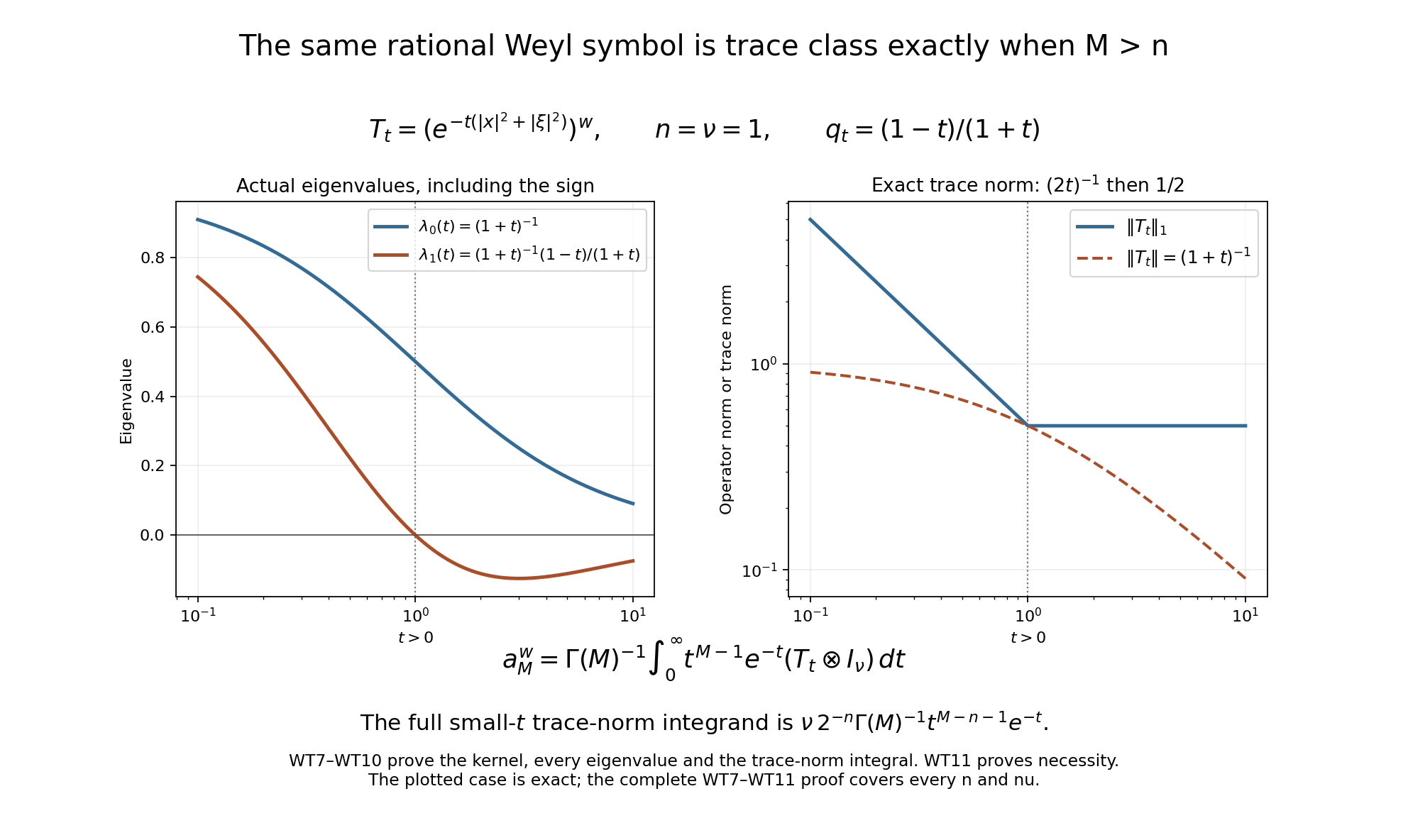
The drawing uses the explicit case $n=\nu=1$. It records the actual sign change of the degree-one eigenvalue at $t=1$ and the trace norm from (WT9), including its factor $1/2$. The rational-symbol classification follows from the full endpoint integral (WT10) and the positive coherent-state integral (WT11), not from a plotted sample. This is an editorial strengthening of the worked example.

11. Exercises and complete solutions

Exercise 1. Let $u\in L^2(\mathbb R^n;\mathbb C^\mu)$ and $v\in L^2(\mathbb R^n;\mathbb C^\nu)$. The rank-one map $S_{u,v}:H_\nu\to H_\mu$ is $S_{u,v}w=u\langle w,v\rangle$, with the lesson’s inner product linear in its first variable. Find its kernel and Hilbert–Schmidt norm. In the square case $\mu=\nu$, find its trace.

Solution. The kernel is the full rectangular matrix $K(x,y)=u(x)v(y)^*$, so $$\iint\operatorname{tr}_{\mathbb C^\nu}(K^*K)\,dx\,dy =\left(\int|u(x)|^2dx\right) \left(\int|v(y)|^2dy\right). \tag{WT4}$$ Equation (CI2) makes this $\|S_{u,v}\|_2^2$. In the square case, the rank-one trace is $\langle u,v\rangle=\int v(x)^*u(x)\,dx$; equation (CI7) gives the same value from the factored diagonal. The answer uses the actual $\nu$-input and $\mu$-output types and does not identify a rectangular operator’s trace.

Exercise 2. Determine every real $s$ for which $H^{-s/2}$ in (CT3) is Hilbert–Schmidt, and explain why $n+1$ is the first integer exponent allowed in the trace-class factorization.

Solution. Equation (CT5) gives $$\|H^{-s/2}\|_2^2 =\sum_{r=0}^\infty \binom{r+n-1}{n-1}(n+1+2r)^{-s}. \tag{WT5}$$ The shell count is bounded above and below by positive multiples of $(1+r)^{n-1}$ for large $r$, so the summand is comparable to $(1+r)^{n-1-s}$. The positive series converges exactly when $n-1-s<-1$, namely $s>n$; at $s=n$ it diverges like the harmonic series. The first integer $s>n$ is $n+1$, exactly the exponent $k$ in (CT6)–(CT13).

12. Antecedent

The proofs above are the course’s direct trace and finite-derivative calculations; the exterior index coefficient and its boundary reduction belong to the subsequent index-formula lessons. The additional differentiation, integration, rectangular-kernel and oscillator-domain inputs are proved in Section 13. The earlier Hilbert–Schmidt and trace-ideal proofs are in Traces that survive passage to cohomology.

13. Complete differentiation and integral inputs

This editorial supplement supplies the vector differentiation step in Section 3 and the scalar integrals in (WT3) and (WT10). It leaves the original symbol, kernel, statements and proofs above identifiable. Its measure and norm inputs are the complete proofs in Banach estimates, quotient spaces and compact parameter arguments, Sections 15.0–15.3, 15.6–15.7 and 17.1–17.3: completed Lebesgue measure, full product integration, compact smooth density, the plane polar formula, and the original Banach-valued integral. No theorem about vector Lebesgue points is assumed.

13.1. A norm-valued differentiation proof

Let $E$ be a real or complex Banach space with its given norm, and let $h:\mathbb R^n\to E$ be strongly measurable and locally norm-integrable. Strong measurability means almost-everywhere convergence of finite-valued measurable functions, as defined in that prerequisite. We prove $$\lim_{r\downarrow0}\frac1{|B_r|} \int_{B_r(x)}\|h(y)-h(x)\|_E\,dy=0 \quad\text{for almost every }x. \tag{TD1}$$ Here $B_r(x)=\{y:|y-x|<r\}$, $|B_r|=r^n|B_1|$, and $0<|B_1|<\infty$; containing and contained coordinate boxes prove the latter two inequalities. The exact scaling is the affine-change formula (LP5). Every average uses the original Lebesgue density. Formula (BI7) constructs its vector integral and bounds its norm by its norm integral; (BI8) permits every continuous linear functional to pass through it.

First, for scalar $g\geq0$ in $L^1$, put $$(\mathcal Mg)(x)=\sup_{r>0}\frac1{|B_r|} \int_{B_r(x)}g(y)\,dy.$$ For fixed radius the integral is measurable by the product-integration proof, applied to $1_{\{|x-y|<r\}}g(y)$. For fixed $x$, it is continuous in positive $r$: the sphere of radius $r$ has measure zero, since its enclosing annuli have measures bounded by $|B_1|[(r+\delta)^n-(r-\delta)^n]\to0$, and dominated convergence applies to $g$. Division by $|B_r|$ preserves this continuity. Hence the supremum can be taken over positive rational radii and is measurable.

We need the following estimate, with its covering constant retained: $$|\{x:\mathcal Mg(x)>\lambda\}| \leq\frac{3^n}{\lambda}\int g(y)\,dy, \qquad \lambda>0. \tag{TD2}$$ To prove it, take a compact subset $K$ of this measurable set. For each $x\in K$, choose a ball centered at $x$ whose average exceeds $\lambda$. These open balls cover $K$, so finitely many suffice. From this finite family choose a ball of greatest radius, retain it, discard every ball intersecting it, and repeat on the remaining family. The retained balls $B_j$ are disjoint. Each discarded ball has radius at most that of the retained ball which removed it. The triangle inequality therefore puts the entire discarded ball inside the concentric ball $3B_j$. Consequently $$|K|\leq\sum_j|3B_j|=3^n\sum_j|B_j| <\frac{3^n}{\lambda}\sum_j\int_{B_j}g \leq\frac{3^n}{\lambda}\int g.$$ There are only finitely many balls here, so no infinite selection theorem is used. The passage from compact subsets to the measurable set follows from the already constructed outer measure, as follows. For a closed bounded coordinate box $Q$, cover $Q\setminus F$, where $F$ is the measurable set in question, by an open $O$ with $|O\setminus(Q\setminus F)|<\varepsilon$. Such a cover is proved in Section 15.0. Then $Q\setminus O$ is compact, lies in $F$, and omits from $F\cap Q$ measure at most $\varepsilon$. Exhaust by boxes and let $\varepsilon\downarrow0$. This proves (TD2) including sets of initially unknown finite measure.

Suppose first $h\in L^1(\mathbb R^n;E)$. Formula (BI4) approximates it in the original norm integral by finite-valued integrable functions. Each nonzero cell has finite measure. Approximate its indicator in scalar $L^1$ by a compact smooth function using (LP11), multiply by its original vector value, and retain the finite sum. The full error is bounded by the sum of the scalar approximation errors times the original vector norms. Thus there are continuous compactly supported $E$-valued functions $h_l$ with $\int\|h-h_l\|_E\to0$. This works even when $E$ is nonseparable.

Write $g_l(x)=\|h(x)-h_l(x)\|_E$ and let $D_h(x)$ denote the nonnegative upper limit of the averages in (TD1). Continuity of $h_l$, the norm triangle inequality and the definition of $\mathcal M$ give $$D_h(x)\leq (\mathcal Mg_l)(x)+g_l(x),\qquad |\{x:D_h(x)>2\lambda\}| \leq\frac{3^n+1}{\lambda}\int g_l(x)\,dx. \tag{TD3}$$ The second term uses the elementary inequality $\lambda|\{g_l>\lambda\}|\leq\int g_l$. These sets are measurable: strong measurability makes $(x,y)\mapsto\|h(y)-h(x)\|_E$ measurable by finite-valued approximation, and product integration and the same rational-radius argument apply. Let $l\to\infty$ at each fixed $\lambda>0$. Every set in (TD3) has measure zero. Taking $\lambda=1/j$, $j\geq1$, proves $D_h=0$ almost everywhere, hence (TD1).

For a locally integrable $h$, apply this argument to $1_{[-L-1,L+1]^n}h$, for each positive integer $L$. It is norm-integrable by the local hypothesis. At $x\in[-L,L]^n$, all sufficiently small balls lie in the larger box, so their original averages agree. The countable union of these boxes proves (TD1) on the original whole space.

For the exact receiver in Section 3, take $E=L^2(\mathbb R^n_z;\operatorname{End}(\mathbb C^\nu))$ with the Hilbert–Schmidt fiber norm, and $h(y)=B(\cdot,y)$. Its original joint $L^2$ kernel makes this an $E$-valued $L^2_y$ function. Here is also its strong-measurability justification. Compact smooth functions are dense in the joint scalar $L^2$ space entry by entry. On their compact boxes, uniform continuity gives finite sums of rectangular indicators times the actual matrix coefficients. Choose such finite tensor sums whose joint squared error from $B$ is summable. Fubini makes their squared $E$-valued slice errors summable for almost every $y$, so they converge there in $E$. Each tensor sum is a finite-valued strongly measurable $E$-valued function of $y$. This proves precisely the required strong measurability; Cauchy–Schwarz on bounded boxes gives local norm-integrability.

Outside the union of the null sets in this construction, (TD1), Fubini and (BI7) give $$\left\|\frac1{|B_r|}\int_{B_r(x)}B(\cdot,y)\,dy -B(\cdot,x)\right\|_E \leq\frac1{|B_r|}\int_{B_r(x)} \|B(\cdot,y)-B(\cdot,x)\|_E\,dy\longrightarrow0. \tag{TD4}$$ Fix also a nonexceptional $x$ for which $A(x,\cdot)\in L^2_z$ and (CI6) holds for almost every $y$. Each matrix entry of its product integral is a bounded linear functional on $E$, by the original Cauchy–Schwarz inequality. Formula (BI8) and (TD4) therefore justify the precise averaging and limit used in Section 3. The continuous representative has its average tending to $K_T(x,x)$. All its entries consequently equal the corresponding entries of $k(x)$ almost everywhere. This proves the full matrix diagonal assertion, its absolute integrability and (CI8), with the existing polar factorization and matrix order unchanged.

13.2. The full Gamma and radial integrals

For real $a>0$, define $\Gamma(a)=\int_0^\infty u^{a-1}e^{-u}\,du$. The integral near zero converges because $a-1>-1$. At infinity, choose an integer $j>a$; the retained exponential-series term gives $e^u\geq u^{j+1}/(j+1)!$, so the integrand is at most $(j+1)!u^{a-j-2}$, an integrable tail. Thus $\Gamma(a)$ is finite and strictly positive. The change $s=cu$, with $c>0$, retains both power and density factors and gives $$\int_0^\infty u^{a-1}e^{-cu}\,du =c^{-a}\Gamma(a). \tag{TG1}$$ For $a,b>0$, apply nonnegative Tonelli to the defining product of these two integrals. In its inner integral use $v=ut$, $dv=u\,dt$; after interchanging the resulting $u,t$ integrals use $s=(1+t)u$, $du=(1+t)^{-1}ds$. These are positive one-variable affine changes on their full positive domains. They give the complete identity $$\begin{aligned} \Gamma(a)\Gamma(b) &=\int_0^\infty\int_0^\infty u^{a-1}v^{b-1}e^{-u-v}\,dv\,du\\ &=\int_0^\infty t^{b-1} \left(\int_0^\infty u^{a+b-1}e^{-(1+t)u}\,du\right)dt\\ &=\Gamma(a+b)\int_0^\infty t^{b-1}(1+t)^{-a-b}\,dt. \end{aligned} \tag{TG2}$$ Every integral before division is nonnegative, so no unproved absolute-convergence interchange occurs. The left side and $\Gamma(a+b)$ are finite and positive; division proves the exact beta value and its convergence. In (WT3) use $a=M-n$, $b=n$, retaining the original condition $M>n$, both powers, and $\Gamma(M-n)\Gamma(n)/\Gamma(M)$. In (WT10) use (TG1) with $a=M$ and $c=1+|x|^2+|\xi|^2$; no matrix or Fourier factor is changed.