Stable modes and the algebra of boundary data
A frozen boundary equation asks which normal profiles remain bounded inside the domain, and which boundary measurements determine those profiles. For systems, the number of profiles counts algebraic multiplicity. Eigenvectors alone can miss solutions. This lesson constructs the bounded solution space from Cauchy data, then changes the equation while preserving that space and its boundary measurements.
Section 13 of Metric and topological foundations proves the full original scalar and finite-coordinate calculus. Its Section 13.12 gives the exact Gaussian, Rayleigh, logarithmic-contour, matrix and half-line receiving maps, retaining every original factor, endpoint and norm.
The complete original real-number, compactness, extrema and finite-norm proofs are in Section 12 of Metric and topological foundations. Its Section 12.10 gives the exact receiving minimum and spectral-contour maps; the original coordinates, norms and constants are retained.
Throughout, vector spaces are finite-dimensional and complex, coefficients are constant in the normal variable, and
We call a solution stable when it is bounded for . Under the no-real-root hypotheses below, this is equivalent to exponential decay of the solution and every derivative. No diagonalizability, simplicity of roots, commutation of matrix coefficients, or prescribed number of boundary equations is assumed.
Polynomial and contour interfaces for stable boundary models proves scalar polynomial division over , Bézout, Cayley–Hamilton, complex triangularization, and the contour moments for globally convergent power-series numerators with specified spectral indices. That lesson now proves the complex-root theorem and the full determinant, kernel and invariant-quotient maps in Section 9. Sections 10.1–10.9 there supply the full finite bases and direct sums, projection rank and trace, matrix algebra, original-inner-product adjoints and operator norms. Compactness of the original unit sphere retains its separate topological base. Section 16 below makes the original annihilator and Cauchy receiving maps explicit. We also use its locally uniform exponential-series calculus, termwise differentiation and integration under uniform convergence, and dominated differentiation of exponentially decreasing tails. The spectral and ODE consequences needed here are proved below.
1. Spectral calculus without an eigenbasis
Let be a finite-dimensional complex vector space and . Choose any norm. The series
converges locally uniformly with all derivatives, since its norms and the norms of its differentiated terms are bounded by scalar exponential series. Thus , , and multiplication of absolutely convergent series gives . If , differentiating shows that it is constant. Consequently
is the unique solution with . In particular the solution space has dimension .
Here is the spectral information, including the nilpotent terms. Keep an original least-degree nonzero annihilator with leading coefficient . Its named monic comparison has factorization ; the original polynomial is , with every unit and multiplicity retained. Section 16.1 proves the full scalar-unit and polynomial evaluation maps. The spectral label used there denotes the same actual root as here, through the identity . The factors are pairwise relatively prime. Repeated Bézout identities give polynomials which are one modulo and zero modulo every other factor. Their sum is one modulo the named comparison, while the full original calculation uses and . Formula (SR2) retains both original scalar factors. Evaluation at therefore gives projections
Their images are exactly
Indeed, the polynomial congruences show both inclusion in this kernel and that is the identity there. Thus . On , write , where . The inverse and the evolution on that summand are
The first identity follows by multiplying a finite geometric series; the second follows from the exponential series for commuting and . The entire-series contour moment formula from the preceding lesson, applied to the first identity, yields
where is a finite union of positively oriented closed contours enclosing every eigenvalue once and no point of the spectrum on the contours. Integrating the resolvent alone around a single eigenvalue gives . These assertions also follow directly from (S2), so multiple poles are included.
The full characteristic/pole comparison is proved in Sections 16.2–16.3, including the exact nonzero leading resolvent coefficient. For later counting, equals the algebraic multiplicity of in . The direct sum decomposes the determinant into the determinants of the restrictions. A nilpotent map is upper triangular with zero diagonal in a basis adapted to its successive kernels; the restriction to therefore contributes . The length of a nilpotent chain affects polynomial factors in time, while the dimension of the whole generalized eigenspace determines the number of solutions.
The exact original annihilator and scalar-unit calculation in Sections 16.1–16.4 proves these same operators and contour formulas with every leading factor shown.
2. A monic equation and its complete Cauchy coordinates
Let have dimension , let , and put
The scalar variable commutes with every coefficient; the coefficients need not commute with each other. The case has only zero solutions and determinant one; the following arguments can be read with .
For , define the companion map
If , its state satisfies . Conversely, the first rows of this first-order equation imply that any state solution is the jet of its first component, and the last row gives . Applying Section 1 proves existence and uniqueness for arbitrary Cauchy data and gives .
We will need the exact characteristic polynomial:
For a direct determinant check, make the triangular change of variables and for ; its determinant is one. The first rows of become , and the coefficient of in the last row is . Move that last block row to the front and eliminate its other entries using the identity block rows. The block-row permutation has sign , and the negative identities contribute . Their product is one. This proves (S5), as a polynomial identity, without assuming that any is invertible.
There is also a useful polynomial encoding of a jet. Set and
This maps bijectively onto the -valued polynomials of degree less than . To see this, read coefficients from the highest power downwards: the coefficient of is , the next is , and in general the next unknown occurs with coefficient , accompanied only by already recovered .
Let be the first coordinate. Solving gives
The latter equality follows by substituting the first formula into the last block row; its coefficient of is . Consequently (S3), applied to , gives the solution with jet :
The contours enclose all roots of . Formula (S7) is valid for repeated roots and matrix poles of arbitrary order. It is the finite sum of the pole moments computed from (S2). The triangular bijection above proves uniqueness of the polynomial in this representation, as well as existence. In particular, it does not require a factorization of into linear matrix factors.
Section 16.7 proves the corresponding original numerator, inverse coordinates, resolvent and contour maps when the actual leading matrix is any invertible . It retains its full determinant and both block signs.
3. Bounded solutions, derivatives, and multiplicity
First, boundedness of a solution of a monic constant-coefficient equation controls all its derivatives. This fact is useful before any spectral separation is imposed.
Lemma. If is any monic matrix polynomial and , then boundedness of on implies boundedness there of for every .
Proof. Write , with state space , and define
If , the continuous integrand vanishes on the interval. Its derivatives at zero then vanish, so every Cauchy coordinate of is zero. The positive function has a positive minimum on the unit sphere. Thus for every ,
All components of the state are bounded. Repeated differentiation of expresses every higher derivative through a fixed power of , proving the claim. The same argument with integration over proves the negative-half-line version. An equation with invertible leading coefficient is first multiplied on the left by its inverse.
Assume now that has no real eigenvalues. Define
where surrounds precisely the upper-half-plane spectrum. This is a projection commuting with . On its image, (S2) shows that and all its derivatives decay as : every polynomial factor is dominated by the exponential . On the image of , the corresponding decay holds as .
Conversely, if is bounded for , set . Then
The norm of on the lower spectral subspace tends to zero, by (S2), while the last factor is bounded. Taking gives . The negative-half-line assertion follows with signs reversed. Hence initial evaluation identifies the two bounded solution spaces with and , and every solution splits uniquely into one of each kind.
For (S4), assume
The companion characteristic identity and the lemma imply that its stable solution space
corresponds under exactly to . All its derivatives decay exponentially. The dimension is the sum of the algebraic multiplicities of the roots of in the upper half-plane. The analogous lower space gives a direct-sum decomposition of all solutions. The statement counts generalized modes, even if the scalar determinant has high multiplicity and the space of ordinary eigenvectors is small.
Section 16.5 also proves the exact bounded modes when real roots are present; those extra modes are distinguished from the original no-real-root decay assertion above.
4. Parameters and fixed projections
Suppose is a family on an open parameter set, where , and every has no real eigenvalues. Near a fixed parameter one can choose the same contours in (S8): invertibility on a compact contour persists under small matrix perturbations. The resolvent is , and, for one derivative,
Repeated differentiation gives finite sums of ordered products of such factors; their order cannot be changed when matrices do not commute. Differentiating the contour integral proves that is . Since the rank of a projection is its integer-valued trace, its rank is locally constant. A basis of its image at one parameter remains a basis after applying nearby projections, so the stable spaces form a vector bundle. A global eigenbasis or a splitting into individual eigenvalue branches is unnecessary.
On a compact parameter set contained in this no-real-spectrum region, there are constants and such that
To justify the common contour used for this estimate, matrix norms give a common bound for all eigenvalues. If their distances from the real axis had no positive lower bound, a convergent sequence of parameters and a convergent subsequence of eigenvalues would give a real eigenvalue at the limiting parameter, by continuity of the determinant. Choose a rectangle enclosing all upper eigenvalues with its lower side strictly above the real axis, and with its other sides beyond the common spectral bound. Its distance from the spectra is positive. Formula (S3) with this contour, and , proves (S11). In parameter charts, derivatives through order obey the corresponding estimate by (S10). Constants are local on the parameter space; no global spectral gap is asserted on a noncompact parameter set.
These results apply to when the coefficients of a fixed-degree monic polynomial vary and (S9) holds. Collisions among roots in one half-plane do not damage the stable bundle or these estimates.
Section 16.6 gives every ordered multiindex derivative with its full multiplicity and the original contour length, spectral-gap and resolvent constants.
5. Collapsing rates within their half-planes
Let , let , and let . Put
Theorem. Each has no real eigenvalues, and its upper spectral projection is exactly . At , its solution with initial value is
Proof. On an original primary summand , the restriction is
Its only eigenvalue has the same strict imaginary-part sign as , including at both endpoints. The fixed direct sum of all original upper summands is therefore the full upper primary subspace for every , and the lower sum is its complementary lower subspace. The spectral projection is uniquely the projection onto the first along the second, hence equals . Formula (S13) follows by exponentiating the restrictions and .
Distinct original eigenvalues can coalesce during this deformation, and at the last endpoint nilpotent parts vanish. Individual generalized eigenspaces labelled by distinct moving eigenvalues therefore need not stay individually identifiable. The two half-plane sums and their projection are what remain fixed.
For parameter-dependent and positive , (S12) has the same regularity as those data by Section 4. There is no additional requirement that avoid the original eigenvalues.
6. Polynomial coordinates adapted to two half-planes
Return to (S4), now with , and fix . Write
There are unique coefficients with
For completeness, set , so and . Then the coefficients are those of the polynomial
This gives an explicit formula
with binomial coefficients outside their ordinary range interpreted as zero. The right side of (S15) has degree at most , proving existence. If a combination in (S14) vanishes, divide by for ; the polynomial vanishes on infinitely many , so each coefficient vanishes. This proves uniqueness and invertibility of the change of basis. Comparing the coefficient of gives
Neither nor , nor any intermediate coefficient, is assumed invertible. The negative powers of in (S16) require ; there is no claim of uniformity as .
7. First-order coordinates that respect decay
For a solution of , define
The polynomials form a basis of the scalar polynomials of degree at most , by the same argument as in Section 6. Thus (S18) is an invertible, constant, scalar-block change from the Cauchy state . There is no loss of a Cauchy coordinate.
The transformed equations are
The second equations follow by commuting scalar polynomials in ; the first is precisely (S14) applied to . We have only moved scalar differential factors past constant matrix coefficients, never exchanged two matrix coefficients.
These equations are exactly a first-order system, not merely consequences that define a larger space. One way to check the converse is to let denote the invertible change in (S18). The leading matrix of the left side of (S19) has row zero , and lower rows have in adjacent columns. Its determinant is one by the factorization in the next result at . Call that leading matrix , and the constant matrix . Every jet initial value yields a transformed solution, so for every initial vector . Hence . Invertibility of proves the converse.
This change of state is an exact first-order reduction. The next construction has a different purpose: it produces a homotopy of fixed-degree polynomial systems beginning with the original equation plus auxiliary equations. Choosing for those auxiliary equations places their characteristic root at , where they have no stable solutions. Auxiliary equations would instead introduce the real root zero.
8. An explicit stabilization and its leading coefficient
For , define the degree- polynomial by its action on . The first component is
and the remaining components are
For , the sum in the middle line of (S20) is empty; the last block appears only once. At the endpoints,
and every entry of contains . After that scalar factor is removed, its equations are (S19).
Let be the coefficient of in . Define by , , and let have identity diagonal, zero off-diagonal entries except in its first row, and
Then
To verify this, its first block is . Its intermediate first-row blocks are , and its last block is . The lower rows are exactly . These are the leading blocks of (S20)–(S21).
Both factors in (S23) are block triangular with identity diagonal. Therefore
Moreover, with , while . Its inverse is the explicit finite expression
In block form, , and for ,
Every entry has degree at most one in the ; using (S17) to replace makes it a linear combination of them. No product of two ’s occurs. The factorization uses only addition, composition with scalar multiples of identity, and the relation (S17). Consequently the inverse calculation also works for coefficients in any unital, possibly noncommutative, algebra satisfying that relation. Only the determinant statement is restricted here to finite-dimensional matrices.
9. A determinant identity retaining every root
For every complex and every ,
Proof. First suppose . The block of rows and columns indexed is lower triangular with diagonal , and therefore has determinant . Eliminating these rows expresses the auxiliary components as
The Schur complement in the first row is
The block determinant formula proves (S27) whenever . Both sides are polynomials in , so equality on that set proves equality also at . The calculation never assumes invertibility of .
If (S9) holds, (S27) proves that is invertible at every real . It also records multiplicity: the upper-half-plane roots, with algebraic multiplicity, are exactly those of ; the auxiliary factor adds only the lower root , with multiplicity . If this is already a root of , multiplicities add. At , writing , where is the first-order polynomial of (S19), gives . A zero of the auxiliary factor is not discarded from the full equation.
10. The stable space is preserved, with an explicit inverse
Assume (S9), and write , with the definition extended to invertible leading coefficient by left normalization.
Theorem. For every ,
is a linear isomorphism. On these spaces,
Proof. The leading coefficient is invertible by (S24), and the determinant has no real zeros by (S27). Section 3 therefore applies to : every stable solution and all its derivatives decay exponentially.
Equation (S21) says . The expression in parentheses is bounded. The kernel of , for , consists exactly of times vector polynomials of degree less than : substitute and use . No nonzero such function is bounded for . Cancellation is therefore valid on this bounded solution space, giving the first recurrence in (S29). Iteration gives the second one.
For , multiply the second identity by . In the last term of (S20), use . The first row of the differential equation becomes
Thus has the asserted codomain.
To construct the inverse, first observe that for a smooth exponentially decreasing function , whose derivatives have the same property, the unique bounded solution of is
Differentiating the integral or integrating once by parts gives , which is equivalent to . The difference of any two bounded solutions is , so is zero. Differentiation under the integral is justified by the exponential derivative bounds. If , then
Every has these bounds by Section 3. Define
These functions are defined on all real ; for fixed , the integration tail still lies in the decaying region. They and all their derivatives decay on the positive half-line, satisfy (S29), and hence satisfy every lower row of . Substituting the recurrences into the first row gives , as above. This proves surjectivity. If , each successive bounded solution of is zero by uniqueness, proving injectivity.
Since commutes with scalar constant-coefficient differentiation on these functions, the lift can also be written
At , this is exactly ; no division by is needed. The same estimates show local dependence of the lift on coefficients and on . In Cauchy coordinates this is an isomorphism of the stable bundles from Section 4. On compact parameter sets, differentiation of (S30) in introduces powers of , whose integrals remain finite because has a positive lower bound and the stable decay estimates are uniform.
11. Boundary measurements, their orders, and the zero endpoint
For , let be a finite-dimensional complex vector space and
The boundary map is
The empty family is allowed, with target zero. We call these measurements complementing precisely when (S33) is bijective. In particular its domain and target dimensions must agree; injectivity alone does not establish complementing data with arbitrary targets.
For any finite orders , composition with (S28) gives
Since is an isomorphism, is bijective if and only if is. This statement includes both and , and does not require .
The preserved data form the commuting square
The left vertical arrow is invertible; the bottom measurement map is invertible exactly when the top one is. This diagram concerns solution spaces, so it does not extend an expression with singular coefficients to arbitrary Cauchy vectors.
For the following alternative expression, impose the additional hypothesis . There are unique coefficients such that
Repeating the change of variables with degree gives
Thus , where
The degrees and powers of follow from (S36), including when the actual order is less than . From (S29),
Consequently for and ,
This is equality of functions of , so it remains true at the boundary after evaluation at zero. The factors make (S37) unsuitable as a formula for an ambient boundary operator at . The correct endpoint map is (S34). On the explicitly lifted stable vectors (S32), the factors cancel with , but this cancellation does not define on arbitrary vectors at zero.
Here the orders are orders in the single normal variable. In a boundary PDE, tangential orders and their Sobolev shifts are additional data. None of the finite-dimensional statements permits dropping them or replacing an arbitrary boundary system by Dirichlet data.
12. The reduction with its leading coefficient retained
Combine the preceding statements under exactly these assumptions: is finite-dimensional over ; ; has degree and leading coefficient ; for every real ; ; and .
The family in (S20)–(S21) begins with the stabilized equation (S22), has no real characteristic roots, preserves the full stable solution space by first-coordinate projection, and preserves bijectivity of every finite collection of boundary measurements transported by that projection. Its leading coefficient has determinant one and inverse entries linear in . The extra boundary expression (S37) requires orders less than and .
Define
It is monic of degree . Left multiplication by the invertible constant matrix changes neither the differential equation’s solutions nor any of their boundary measurements. Because , it also leaves (S27) unchanged. At , (S23) gives , so the starting polynomial is unchanged. At ,
for a matrix with no real eigenvalues: the first-order factor is monic and its determinant is . Thus its stable equation can be further deformed by Section 5. The scalar factor in (S39) has only the lower root ; cancellation of that factor is valid for bounded solutions by Section 10, and is not an equality of full solution spaces.
The preceding construction begins with a monic polynomial because its Cauchy coordinates use the leading identity. For an original polynomial retain and every leading-coefficient factor. Set only to calculate the monic comparison, and let and denote (S20)–(S23) formed from . The expression is used only for this comparison; multiplication is on the left. The family attached to the original equation is Its first row has the original left factor ; the other rows are unchanged. In particular, The determinant identity follows without cancellation: , while left multiplication contributes . The leading matrix is These orders follow from matrix multiplication; no commutation of with the other coefficients is used. Since the diagonal left factor is invertible, if and only if , and if and only if . Thus the first-coordinate stable isomorphism and every transported boundary measurement remain exact for the original equation. The monic comparison satisfies ; it does not erase from the original family. For singular , this comparison is unavailable and the full -dimensional Cauchy space can fail, as Problem 6 shows.
13. Example: cubic time factors in a four-dimensional stable space
Let , let , and consider
It is monic of degree two, and its determinant is , so every solution is stable. To see all four coordinates directly, write
Since , substitution proves the equation. The free constants give all four solutions by Cauchy uniqueness. Thus a second-order matrix equation can contain a cubic polynomial times an exponential; the order of the scalar equation alone does not bound the length of a generalized chain for the full state matrix. In agreement, the upper-right entry of is .
The pair of measurements , is complementing because every Cauchy jet is stable. Under the construction with , the stabilized system has determinant . Its stable dimension remains four, while its total solution dimension is eight.
14. Example: noncommuting coefficients and an unsuitable trace
Consider
Its coefficients and do not commute: has upper-right entry . The determinant is . A bounded solution must have , since its second component solves . Therefore
The stable dimension is two. The ordinary vector trace has image and a one-dimensional kernel, despite equality of source and target dimensions. In contrast, the two scalar measurements
are bijective onto . The entire construction above applies without changing the coefficient order or imposing a scalar boundary model.
15. Problems with solutions
Problem 1: a real root at the boundary of the hypothesis. Let , for real . Determine the positive-half-line bounded initial values, including . Explain the failure of a continuous stable projection across zero.
Solution. The solution is . For , every initial vector is stable. For , only zero is bounded. At zero, precisely vectors with are bounded, and their solutions are constant. Thus the bounded dimensions are respectively two, zero, and one. The upper spectral projection is for positive and zero for negative , so cannot extend continuously across zero. At zero, boundedness does not imply decay, and the upper/lower splitting omits the real generalized eigenspace. This identifies why the no-real-spectrum hypothesis is used.
Problem 2: the smallest block homotopy. For , write , its leading coefficient, and an inverse of that coefficient. Verify the determinant-one assertion without commutativity assumptions.
Solution. With ,
Writing , its leading coefficient and inverse are
Multiplying the two displayed factors or multiplying verifies the formulas; no two unrelated coefficient matrices are interchanged. Each triangular factor has determinant one. In addition, (S27) reads .
Problem 3: boundary orders beyond the coordinate basis. Let have arbitrary finite degree and let be monic of degree . Prove a unique division formula with . Which factor order is required, and what does this imply on solutions?
Solution. If has leading term with , subtract . The leading term cancels because , and the degree decreases. Iterating constructs and of degree below . If two decompositions exist, a nonzero difference of degree makes have degree exactly , since its leading coefficient is unchanged by multiplication by . It cannot equal a polynomial of degree below ; hence both differences vanish. The required order is , which composes . On constant-coefficient solutions, . This justifies normal-order reduction for this algebraic model. A PDE with variable coefficients or tangential orders needs its own division and mapping argument.
Problem 4: a negative power of the homotopy parameter. Take , , and any stable scalar solution . Find , verify (S37), and identify its valid zero-parameter interpretation.
Solution. Since , one has . For , the recurrence gives , so . At zero, the stable lift has ; inserting this into is undefined. The correct boundary functional remains from (S34). Along a lifted family, its limiting value can be computed before setting , using . It is not an ambient formula at zero.
Problem 5: nilpotent coalescence at the last endpoint. Let be the direct sum of the blocks on , on , and on , where . Describe (S12) when .
Solution. The first block is , the next is , and the last is . The upper projection is always . For , the first and second upper blocks have distinct eigenvalues; at one, their eigenvalues coalesce at and the nilpotent part of the first vanishes. The full -eigenspace at one has dimension three. Thus individual primary summands associated with distinct spectral values have merged, while the upper spectral subspace has remained the same three-dimensional space throughout.
Problem 6: why the leading coefficient matters. Treat as a degree-one matrix polynomial on . Determine the solutions and compare their dimension with the formal count .
Solution. The equations are and , so the solution space is one-dimensional, although . The leading coefficient is , which is singular. Initial values are constrained, and multiplication by the inverse leading coefficient is impossible. In contrast, a genuinely monic degree-one polynomial supplies two free initial coordinates. This example concerns the leading-coefficient hypothesis; its determinant also has a real root, so it is not an example within the stable reduction theorem.
16. Full original factors in the spectral and Cauchy maps
We make explicit every scalar and matrix leading factor used by Sections 1–5 and 12. The original characteristic multiplicities, nilpotent orders, projection maps, Cauchy coordinates and contour conventions remain in the calculation. The bounded-mode classification at real roots and the complete original-leading-matrix numerator map are stated as additional results; they do not silently change the no-real-root assumptions of the earlier reduction.
The entry proof is Polynomial and contour interfaces for stable boundary models, Sections 2–4 and 9: original polynomial division and Bézout, full complex roots/factorization, original scalar units, determinant signs, kernel coordinates and both invariant quotient maps. We retain the finite basis and scalar-calculus entry definitions used there. Each argument below preserves the chosen original norm and actual coordinates; no Jordan decomposition or selected smooth eigenvalue branch is assumed.
16.1. The original annihilator and complete primary projection maps
Let be the original finite-dimensional complex vector space, , and . Cayley–Hamilton in Section 4 of Polynomial and contour interfaces for stable boundary models supplies a nonzero annihilator. Keep an original least-degree nonzero annihilator , with original leading coefficient . That lesson proves that divides every annihilator. For , is nonconstant, because a nonzero constant acts as that nonzero scalar times the nonzero identity. The full factorization proved there is Every original leading unit and root multiplicity is retained. A least-degree choice is unique up to its nonzero original scalar unit, by division in both directions. The named monic polynomial is exactly , as a comparison; it does not replace in this calculation.
The coprime-factor proof in Section 3 of Polynomial and contour interfaces for stable boundary models gives . In the original quotient calculation set . The full identities are For the factor , is one modulo that factor; for every other factor it is zero. Thus each of , , and for is divisible by every factor. The exact Bézout divisibility proof in Section 3 of Polynomial and contour interfaces for stable boundary models makes it divisible by their full product . Its evaluation is zero because . Consequently Here the image equality is an exact map: gives the first inclusion; gives on the kernel. Applying to a zero sum proves directness. Each projection commutes with , since it is an evaluated scalar polynomial.
A different Bézout choice has the same factorwise remainders. Its difference from is a multiple of , whose full evaluation is zero. Thus it gives the same actual , not just the same abstract summand. Under an original coordinate change , polynomial evaluation gives : expand every finite power and use the ordered adjacent products . Applied separately to both factors in (SR2), this gives This is the exact coordinate map for the full original projection.
If , a least-degree annihilator can be the original nonzero constant . Its root set is empty, and the empty projection sum is zero, exactly the identity of the zero vector space. The empty decomposition in (SR3) therefore includes that case without adding a root or assigning a multiplicity.
16.2. Actual nilpotent order and characteristic multiplicity
On define the original restricted operator . Equation (SR3) gives . In fact every is nonzero and this exponent is exact.
To prove both assertions without a Jordan assumption, suppose that , also including an empty . The original polynomial would annihilate by that supposed zero power. It annihilates every other through the retained full factor . The direct sum (SR3) would then make it an annihilator of , with its original nonzero leading coefficient and degree one less than . Minimality excludes this. Hence ; in particular .
Choose an actual for which . The original vectors are independent. If their linear combination vanished, take its smallest index with nonzero coefficient and apply . The full higher terms vanish by the known zero power, leaving that nonzero coefficient times the unchanged nonzero vector , a contradiction. Thus
For the full determinant calculation choose a basis by successively extending bases of for . The actual map sends each such space into the preceding one. In that ordered basis its matrix is upper triangular with every diagonal entry zero; no vector or matrix entry is rescaled. For the full original change of basis , the determinant identities proved there give Choose bases of the original direct summands and concatenate them, with full coordinate matrix . The original operator is block diagonal in those coordinates. Its full characteristic polynomial is therefore All determinant factors remain explicit and their inverse products are proved; the characteristic leading coefficient one was computed from the original permutation sums in the polynomial and contour lesson, rather than imposed on the original annihilator. Each root’s characteristic multiplicity is exactly , while the annihilator exponent is exactly . The opposite determinant convention retains the full factor .
An eigenvalue is a root of : if , , then the original finite polynomial gives . Conversely each has a nonzero vector in , for example above. Thus is precisely the original spectrum. For , both spectra are empty and the actual characteristic determinant is the empty product one.
16.3. The original resolvent, pole orders and every unit factor
For , multiplication of the full finite geometric sum gives on the original summand Indeed multiplication by produces the identity minus , and that full terminal term is zero by (SR3). The product in the opposite order is the same since every factor is a power of the same original restricted operator. Using (SR2)–(SR3), the full global operator formula is Every actual scalar-unit and projection factor is present. Acting on each original summand proves both inverse identities for this original matrix; no leading coefficient has been dropped from the receiving map.
Multiplying (SR10) by the full power and taking gives All terms with a smaller pole power at tend to zero; every term at a distinct root has a bounded nonzero denominator near and also tends to zero after that multiplication. The nonzero conclusion follows by applying the right side to the unchanged from Section 16.2. Hence the resolvent’s pole order is exactly , which need not equal the characteristic multiplicity . This is an exact nonzero coefficient and limit, not merely a distinction between two names.
For example, in the original three coordinates let Direct multiplication gives both inverse identities and all displayed zeros. The full determinant is . An original least-degree annihilator is , for any original : the actual nilpotent part has square zero and is nonzero. A nonzero degree-zero annihilator is impossible; a degree-one annihilator would have to vanish on all diagonal entries, leaving its nonzero leading coefficient in the actual upper-right entry, also impossible. Thus the characteristic multiplicity is three and the exact annihilator/resolvent order is two.
16.4. Original contour and exponential receivers at every order
Let be a finite integer linear combination of the original piecewise closed paths, avoiding every root. Keep For a numerator having its asserted globally convergent power series about each of these finitely many roots, the proved entire-series moment formula of Polynomial and contour interfaces for stable boundary models gives the full receiving identity This follows by integrating the actual finite sum (SR10). No sum/interchange beyond the proved scalar moments is needed. Every factorial, root repetition, nilpotent power, contour index and original projection factor remains. The stated entire-series hypothesis includes constants, polynomials and exponentials. No formula for an arbitrary holomorphic numerator on an arbitrary domain is inferred here.
For , all higher derivatives vanish exactly; a contour with index one at precisely the selected roots and zero at the others therefore gives the sum of their actual . For , the original derivative is , so (SR14) retains all powers of and every factorial.
The corresponding exponential equality is obtained directly from the original operator series, without a contour assumption: On each original , the two operators and commute. Expand every finite binomial power of their sum. The scalar exponential majorants give absolute convergence on each compact time interval, including the differentiated series, so regrouping by the finitely many surviving powers is valid. The full factorial relation gives the two series product. All higher nilpotent terms are the proved zero operators, not omitted nonzero contributions. Acting on the full direct sum proves (SR15).
Termwise differentiation of the actual series gives , where , and repeated differentiation gives . The original addition identity gives . Thus every solution of is , because differentiating the full product gives zero. Initial evaluation and are inverse linear maps; these are the actual Cauchy maps used in the source.
16.5. Complete bounded-mode classification, including the real roots
First every linear map is bounded for the original chosen norm. Choose an actual basis , retaining these vectors. If , triangle inequality and Cauchy–Schwarz give , with the full constant . On the coordinate unit sphere the actual function is continuous by that inequality, and is everywhere positive by independence. Coordinate compactness supplies its actual minimum . Homogeneity then gives . For any original linear map , this proves Every original basis vector and both comparison constants are retained. These are comparison maps, not replacements of the original norm. In particular all projections and coordinate functionals used below are bounded. The zero-dimensional case requires no positive sphere minimum and every map is the zero map.
On , (SR15) gives for an actual For every full term tends to zero as . To prove the elementary exponential domination, choose any . The scalar series gives for , so . The remaining factor is bounded and tends to zero. Every derivative is covered by the same actual finite expansion with the additional fixed factor .
Conversely take and the largest for which . It exists and lies between zero and . Some actual coordinate functional has ; boundedness was proved in (SR16), without changing or . The complete scalar polynomial in has nonzero leading coefficient . For , the full reverse triangle inequality bounds its modulus below by If , the lower sum is at most times its full coefficient sum. Taking at least twice that coefficient sum divided by the actual nonzero leading modulus makes (SR19) at least half the full leading term. If , the lower sum is empty and the modulus is its exact nonzero constant.
It follows that when , every nonzero gives an unbounded solution on the positive half-line, since its scalar lower bound contains . When , it is bounded exactly when , equivalently ; then the solution is exactly . On a general , applying the bounded actual projection to a bounded solution isolates each such component; components cannot conceal one another’s growth. Thus the complete positive-half-line bounded initial space is With , , the same full expansions and inequalities reverse the imaginary-part signs, giving These formulas prove the precise additional real-root modes rather than simply discarding the no-real-root hypothesis. Under the original no-real-spectrum assumption in Section 3 the extra sums are empty, so its actual upper projection gives , its lower projection gives , and every such solution and derivative decays in its own half-line. The original stable dimension counts in the upper half-plane, by (SR8), whereas time-polynomial degree is bounded by . Neither count can be substituted for the other.
16.6. Full ordered parameter derivatives and common contour bounds
For an original family , near a fixed parameter a compact contour avoiding its spectrum stays disjoint from nearby spectra. Indeed the original determinant is continuous on the compact contour, has a strictly positive modulus minimum there, and small changes of its full finitely many coefficients preserve half that minimum. Inversion is continuous through its full cofactor matrix divided by that nonzero determinant. Differentiating and multiplying by the actual inverse gives , with this exact product order.
For a nonzero multiindex , , the full formula is Here every inner list is ordered; matrices are never commuted. One direct proof retains the actual Neumann series for the original difference small enough that its operator product norm is less than one. Its finite Taylor coefficient at is the sum over ordered nonzero lists in (SR22); each coefficient is divided by , and differentiation multiplies it by the full . Terms with more than differences have no such coefficient. The remainder bounds in the finite Taylor theorem and the geometric-series tail make the coefficient passage valid through order . Equivalently, labeling each of the successive derivative applications partitions the labels into ordered nonempty batches; their multinomial counts are precisely the displayed coefficients. Both constructions include every repeated derivative and every original factor.
For a compact parameter set with no real spectrum, the original norm has a common bound for , and every eigenvalue satisfies by the original eigenvector inequality in Section 9.8 of Polynomial and contour interfaces for stable boundary models. A hypothetical sequence of spectral points whose imaginary parts tend to zero has a convergent parameter subsequence and a bounded complex-point subsequence. Continuity of the original full determinant would give a real eigenvalue at the limit, contradicting the original hypothesis. Thus there is an actual gap .
Choose an original positive rectangle enclosing all upper roots, with lower height , upper height greater than , and left/right coordinates beyond . Its orientation and all its edges are retained; the proven rectangle index is one at every upper root and zero at every lower root. Let be its full length and let . This is finite by the original determinant/cofactor continuity and compactness. The original contour formula therefore gives The full contour factor yields in the norm bound, and retains the original differential convention.
For each parameter derivative in a fixed original chart, insert every term of (SR22) into the same contour. Its original operator norm is bounded by For the actual bound is (SR23). The finite derivative bounds hold in each chart on the compact set under consideration. This proves the full regularity and uniform decay statements in Section 4 even when roots collide in one half-plane; no selection of individual smooth roots was used. It makes no global gap claim on a noncompact parameter set.
16.7. Original matrix-polynomial Cauchy and numerator maps
In this section has the original meaning in Section 2 as matrix-polynomial order. Keep , with , , and all original matrix coefficients in their original order. If , all state spaces and solution spaces are zero and every determinant is the empty product one. Otherwise let . The actual original-equation companion and jet maps are The original equation implies through its last row after multiplying on the left by the displayed . Conversely the first rows give every jet coordinate from the first, and multiplying the full last row by the original gives exactly . Both implications retain every left factor and do not commute any coefficients. Therefore the actual map is inverse to , by the already proved first-order uniqueness; the original solution dimension is .
For a direct characteristic calculation make the original triangular coordinate change , , on the state coordinates. Its original block diagonal is all identities, so its determinant is one. The first output rows of are . The coefficient of in the last row is exactly , with this order. Move that last block row to the front: its full sign is . Each remaining negative identity gives the total factor . Eliminate every other entry of the first row by those identity rows, retaining the original determinant under each row addition. Thus Both signs are retained and their product is one because their full exponent is , an even integer. Also by the original determinant multiplication proof. Hence the nonzero original prefactor preserves every root and multiplicity through an explicit scalar-unit map. It is not a replacement of the original determinant. All formulas include , where the negative block list and row permutation are empty.
The full original polynomial numerator of an arbitrary actual state is Here is the original invertible leading matrix, including at the highest coefficient . The inverse map from the full numerator coefficients is the ordered triangular recursion For the sum is empty. To verify each row, the coefficient of in (SR27) is ; its last term is precisely . Multiplication on the left by the actual inverse yields (SR28). Thus the original numerator map is a linear bijection, with every matrix order and leading factor explicit. Its monic comparison has ; the comparison does not erase from either actual forward or inverse map.
To find the first coordinate of the actual resolvent solve . Its first rows give For the last row, multiply by the original and substitute all preceding rows. Its right side becomes the full sum . For each original , its coefficient is exactly , proving the second identity. All denominators are legitimate exactly away from the original roots by (SR26) and the actual determinant-inverse criterion; no linear factorization of a matrix polynomial has been assumed. Applying the already proved exponential contour receiver to the original gives Every root multiplicity, matrix pole order, original leading factor, factorial in the earlier scalar pole moments and the original contour prefactor is retained. This is the full original-equation receiving extension of the monic formula (S7) in Section 2; its arbitrary numerator is unique through (SR28).
Boundedness of the original first component gives boundedness of the full original state without assuming spectral separation. With the original state and component norms let . If , continuity makes its integrand zero on the entire interval. The first-coordinate solution is then identically zero there. Its derivatives at zero vanish, and its Cauchy coordinates vanish by the first rows of (SR25). Thus is positive on the original nonzero state space. Its continuity follows from the original finite matrix exponential and norm bounds; the original unit sphere is compact by the retained coordinate comparisons (SR16). Let be its actual minimum on that sphere. Homogeneity and the original flow addition rule then give Hence a bounded has a bounded original jet; conversely its first-coordinate projection is bounded whenever its jet is bounded. The exact derivative conventions are and , retaining the full original factor . The actual finite operator norm bounds prove boundedness for every derivative. The negative-half-line proof uses the original interval with its own positive minimum and the same exact Cauchy map. For the zero state space the implication is immediate and no minimum on an empty sphere is introduced.
When the original determinant has no real roots, (SR26), (SR20)–(SR21) and (SR31) identify the original bounded solution space with the companion’s upper primary space and prove decay of every derivative. Its dimension is the sum of the upper-root algebraic multiplicities of the original , with the original map displayed in (SR26). The full leading-coefficient homotopy and transported boundary measurements in Section 12 retain their separate original formulas and proofs. Formulas (SR25)–(SR31) give the complete original-equation Cauchy, numerator, resolvent and contour maps without dropping its leading matrix.
17. Bounded profiles with complex parameters
This separate extension allows real characteristic roots and complex stabilization parameters. Sections 3–12 keep their original stable, no-real-root statements. Here bounded profiles may contain nondecaying real-root modes. The complete classification and jet estimate in Sections 16.5 and 16.7 provide the additional argument; no uniform bundle claim through a real-root crossing is made.
17.1. The original polynomial and its full stabilized family
Keep the original finite-dimensional complex space, its chosen norm, and There is no restriction on the real roots of . Fix Use only for the coefficient calculation (S15)–(S17), retaining the original polynomial. Those identities use , scalar polynomial algebra and the actual ordered coefficients; their proofs hold for complex without a positivity assumption. Form by exactly (S20)–(S21), with every displayed power of , including the empty middle sum when . The original family and leading coefficient are Indeed the factorization (S23) is still . Its actual nilpotents satisfy , , so (S25)–(S26) is the same finite inverse for every complex . Both triangular determinants equal one. This proves (SB3), keeping the inverse product in its required order.
The lower-block elimination in Section 9 also uses no real-parameter restriction. For it has the same lower-block determinant and the same Schur complement . Thus, with both original determinant factors visible, Both sides are polynomials, so the identity holds also at . The auxiliary root is , with imaginary part and multiplicity . If it is already an original root, the multiplicities add. Every original real root remains in the determinant, with its full algebraic multiplicity.
17.2. The bounded inverse and all original derivative bounds
Let consist of smooth solutions of the original equation on that are bounded for ; define in the same way. They include all bounded real-root modes. By (SR31) and (SB3), boundedness of either solution controls its complete original Cauchy jet and every derivative. This implication requires neither spectral separation nor exponential decay.
If is smooth on and all its derivatives are bounded on the positive half-line, set For negative , split this integral at . Its first part is over a finite interval of smooth values; its tail has the same exponential majorant as on the positive half-line. On a compact set of ’s the finite interval can be chosen uniformly. This proves convergence and justifies every differentiation in by the corresponding derivative majorant.
To verify the equation, integrate the derivative of . The upper endpoint is zero, the lower endpoint is , and consequently . Including the original factor gives , hence . Two bounded solutions differ by . Its norm is , so boundedness forces . Thus (SB5) is the unique bounded inverse. It commutes with each , by the just-proved differentiation.
For , retain the actual constants , . Direct integration yields In particular gives the full bounded, nondecaying case with denominator .
Theorem. For every parameter pair (SB2), first-coordinate projection is a linear bijection Its inverse is exactly If for all required derivatives, then the lifted components satisfy For , the single summand is the original bound.
Proof. For a bounded original family solution the lower row says , where . All its derivatives, and thus , are bounded by (SR31). Substituting gives . Thus is a vector polynomial of degree at most . If it is nonzero, an actual bounded coordinate functional detects a nonzero leading coefficient. The full polynomial lower bound (SR19), multiplied by , is unbounded. Therefore . This proves every recurrence (S29) on the present bounded space, including complex .
Substitute these recurrences in the original first row. Its complete expression is The last summand uses the additional in (S20), exactly as in Section 10. This proves the codomain of (SB7).
Conversely, (SR31) bounds every derivative of a bounded original , so each step (SB8) is defined by (SB5), has bounded derivatives by (SB6), and satisfies the actual lower row. Equation (SB10) gives the first row. This proves surjectivity. Uniqueness of the bounded inverse successively shows that a lifted solution with has every component zero, proving injectivity. In particular gives with no division by that parameter.
Finally and (SB6) give the recursion for the derivative bounds . Starting at , its two finite sums combine by , with each endpoint term retained. Induction proves exactly (SB9).
17.3. Exact iterated kernels and parameter derivatives
The lift has a full integral formula, rather than only a formal inverse power. For , Induction proves this formula. The step from to has an absolutely integrable double integral, bounded on the positive half-line by the complete product envelope . For negative , use the same finite-interval/tail split as above. Fubini therefore applies. The substitution , with Jacobian one and , has inner integral . The factor becomes exactly , proving (SB11) with its full factorial.
Only scalar constant-coefficient operators are commuted in the following binomial calculation: Indeed commutes with , and expansion of supplies precisely these coefficients. No two original matrix coefficients are commuted.
For each integer , differentiation in gives and On a compact subset of , the displayed integrals have common integrable derivative envelopes, which justifies the differentiation. The scalar moment used here is exact: for , . At it is direct integration. For , integration by parts has zero upper endpoint and zero lower endpoint, and gives times the preceding moment. This proves every factorial in (SB14).
For the full product rule for the original lift is Its indices make every factorial and power defined; differentiated polynomial terms outside this range are zero. Taking norms and using (SB14) proves the explicit bound Here by (SB2), and every power-zero factor equals one. For the other parameter, the complete formula is At the power-zero term is one. The coordinate is independent of both parameters; its positive-order parameter derivatives vanish. Applying (SB17) to (SB15) gives all mixed derivatives, with exactly the same finite product-rule coefficients.
For fixed and , these formulas prove holomorphic dependence of the lift on in its right half-plane and polynomial dependence on . To verify the analytic assertion directly, expand in (SB5) at a fixed . For , the sum of integral norms in any bounded derivative seminorm is at most . It converges, so termwise integration gives the Taylor series in that seminorm. On a compact negative interval, the finite first part has uniformly bounded smooth input values and an entire exponential series; the remaining tail has the same convergent majorant, with its finite shift factor. This proves the assertion in each local derivative seminorm as well. Formula (SB11), finite products and (SB12) then give the asserted dependence of every component. This concerns a fixed original solution space; it does not assert smoothness of bounded spaces when an original root crosses the real axis.
17.4. Real modes, multiplicities and the exact Cauchy maps
For the original companion in (SR25), the bounded initial space is exactly Only actual roots contribute a summand. Formula (SR20) proves this for the full state and (SR31) identifies first-coordinate boundedness with state boundedness. The original Cauchy map and its inverse in (SR25) identify it with the actual solution space.
The exact real-root kernel map, for each real , is The first rows of the eigenvector equation force precisely these coordinates. The last row, multiplied on the left by the actual , says . Both directions follow, proving the map and inverse without dropping the leading coefficient. Formula (SR26) retains its complete signs and factor ; hence every upper-root primary dimension equals the algebraic multiplicity of that root in the original . Consequently Real bounded modes are counted by their geometric nullities, not by substituting their entire algebraic multiplicities. Higher real Jordan terms give the unbounded time polynomials already proved in (SR18)–(SR20).
For real , , since its imaginary part is . The original stabilized real-root kernel and its inverse are The lower rows uniquely force these coordinates because ; the first row is the actual Schur complement proved in (SB4). This proves the displayed bijection. For , direct integration in (SB5) gives , and . Thus (SB8) gives exactly the coefficient in (SB21), preserving the original frequency and factor . At , its first coordinate is one times , and every positive-index coordinate is zero. The auxiliary lower root supplies no additional bounded mode by the classification (SR20).
17.5. Every finite boundary measurement and its ordered remainder
For the original finite family (S33), with arbitrary finite normal orders, put The target remains the actual , including the empty target. The bijection (SB7) proves and : the first follows by evaluating (SB22), and the second follows in both directions using the inverse lift. Thus bijectivity, kernel dimension and image are preserved for every complex , including zero, and every in (SB2).
When , equations (S35)–(S36) retain exactly their full coefficients, including , , , and the entire signed binomial sum. The polynomial change of variables needs only , so applies here. The same recurrence proves (S37) for as an equality of functions on the lifted bounded space. It remains unsuitable for an ambient operator at zero; (SB22) is the actual endpoint map.
For any larger boundary degree one can also prove an exact polynomial reduction without altering the original equation. If its current leading coefficient is and its degree is , subtract This cancels exactly the leading term , with the original composition order. Repeating the strict degree decrease gives , where . Uniqueness follows because any nonzero difference , with leading coefficient , gives the nonzero leading coefficient in ; invertibility of makes its degree at least . It cannot equal a polynomial of degree less than . On actual solutions, constant-coefficient differentiation and these ordered compositions give . Thus the actual arbitrary-order measurements can be computed by this remainder and the original coefficient formula (S36), with every subtracted term recorded. This finite-dimensional normal-variable proof makes no reduction of tangential PDE orders or their Sobolev shifts.
17.6. The exact measurement map during rate deformation
Return only for this paragraph to the original no-real-root branch (S9). Let be the original companion, its full upper projection, and a fixed real number. The deformation in Section 5 is Its bounded initial space is the same , by (S12). An original profile is ; the new first-order state profile is , for the same . Sending to is a bijection: its forward map uses the unique original Cauchy state, and its inverse is . First-order uniqueness and (SR25) prove both compositions to be identities.
For the original boundary polynomial, keep every original coefficient and derivative order in Since , this is precisely the transported original measurement. Its commuting map is proved by substituting , so it preserves the original kernel, image and bijectivity.
If one instead applies the unchanged polynomial to the first coordinate of the new state profile, the measurement is . The complete difference from (SB25) is For each , expansion of the middle difference produces . Successive terms telescope, retaining their order, to . This proves (SB26) without assuming commutation. The zero-order summand has zero difference; for degree zero the displayed sum is empty.
A concrete original order-two example shows why this receiving map matters. Take Here , , and belongs to the bounded upper space. The original measurement and its transported value are both . Applying the unchanged derivative polynomial to the deformed first coordinate instead gives , with difference . Both profiles are exponentially decreasing. This proves that preservation of the initial stable space does not itself preserve unchanged derivative expressions; (SB25) supplies the exact correspondence. The earlier stable-bundle statement is retained with its original scope.
17.7. A real double root and an exact complex lift
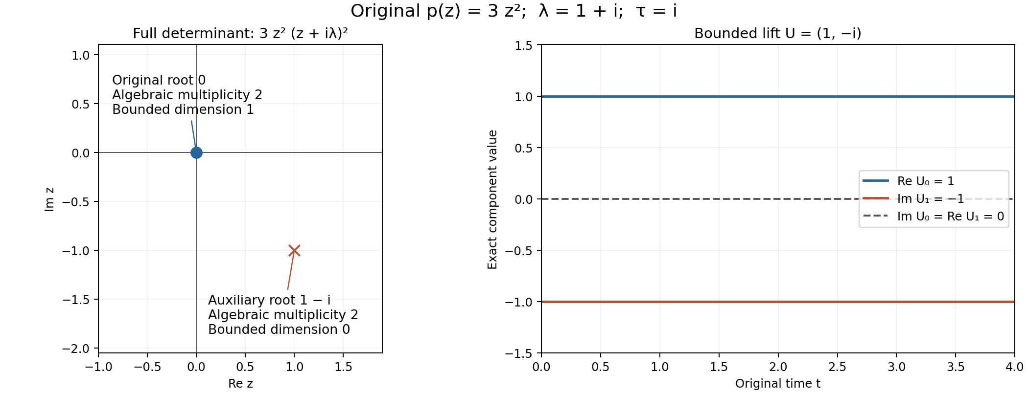
The figure uses the original polynomial , , , , . The coefficient calculation gives , since . The full original determinant is The original root zero has algebraic multiplicity two, but its bounded original space consists exactly of constants and has dimension one: gives , bounded exactly when . The auxiliary root also has multiplicity two and has no bounded positive-half-line mode. Formula (SB21) gives the exact lifted constant . The original first-row value at is , while the lower row is . These are symbolic equalities with all factors retained. The right panel shows , , and both zero components. Its finite plotting interval is an illustration of this exact profile, not a numerical proof of boundedness. The editable figure source and parameters preserve these original coordinates.
If , both solution spaces and all kernels above are zero, every determinant is the empty product one, and every measurement has the zero-domain image. The proofs use no minimum on an empty sphere. All statements about nonzero leading coordinates and roots then disappear, while the zero-space bijections and arbitrary target convention remain exact.
Further questions and analytic use
The next analytic use of this algebra is a family over nonzero tangential covectors. Section 4 supplies its stable vector bundle, and (S33) supplies the finite-dimensional complementing map. A global boundary parametrix also needs symbol calculus, coordinate invariance, bundle gluing and adjoint theory; Cauchy data from jumps and residues and Solving an elliptic system from compatible boundary measurements develop those analytic steps. A fiberwise stable isomorphism alone does not establish their Sobolev estimates or index statements.
For the analytic use of a homogeneous differential principal polynomial, Cauchy data from jumps and residues, Section9 proves the exact reflection of the original solutions and every Cauchy jet. Its positive mode bundle together with the antipodal pullback of that bundle maps bijectively onto the entire original jet bundle, with an explicit inverse. In dimension at least three the original stable rank is necessarily half the total solution rank; in dimension two the antipodal ranks are complementary and may differ. These conclusions use the additional homogeneous differential and ellipticity hypotheses proved there. They are not imposed on the arbitrary matrix polynomials or bounded real-root constructions of this lesson.
Two useful research questions are to identify when the stable bundle admits a globally chosen system of boundary measurements, and to determine which additional estimates survive when spectral roots approach the real axis. The examples here already distinguish the local rank condition from a global choice of boundary data, and show why estimates uniform through a real crossing cannot be inferred from this lesson.
References
The finite-dimensional algebra, decay estimates, examples and solved problems in this lesson are given above.
Polynomial and contour interfaces for stable boundary models, Sections 2–9, proves the exact scalar algebra and contour tools used here.