Two p-adic logarithms: determinant bounds
Draft. Public domain (CC0).
A large valuation of \(2^a-3^b\) means that the two powers agree to many p-adic digits. The determinant method measures how far this agreement can continue. It places products of powers in a single residue class, obtains a nonzero algebraic determinant, and compares a height bound with the large valuation forced by near agreement.
We use the exponential, logarithm, power laws and cyclotomic distances proved in p-adic analysis for linear forms in logarithms. The polynomial zero argument is the method proved in Two logarithms I: interpolation determinants. The weighted product formula is Places of number fields in extensions and the product formula, Theorem 5.2. The height convention and its power law are proved in Heights of algebraic numbers. The necessary determinant estimates are written out below.
Throughout, \(v=v_p\) is normalized by \(v(p)=1\), and \(\ln\) is the real natural logarithm. All algebraic numbers have a specified embedding into \(\overline{\mathbb Q}_p\). We distinguish the global degree \(d\), local ramification index \(e\), and local residue degree \(f\).
1. Residues and principal units
Put \(K_0=\mathbb Q(\alpha_1,\alpha_2)\), \(d=[K_0:\mathbb Q]\), and \(F=\mathbb Q_p(\alpha_1,\alpha_2)\). Its residue field has \(p^f\) elements and \([F:\mathbb Q_p]=ef\le d\). Assume \(v(\alpha_i)=0\).
The multiplicative group of the residue field is cyclic. Here is an elementary proof. In a finite abelian group, elements whose orders have prescribed prime power parts can be multiplied to obtain an element of order equal to the least common multiple \(m\) of all element orders. To see this, for each prime choose an element whose order contains the largest occurring power of that prime, and raise it to its complementary part; the resulting elements have pairwise coprime orders. Their product has the product of those orders, since a power that kills the product must kill each component. In a finite subgroup of a field's multiplicative group, every element is a root of \(X^m-1\), so the group has at most \(m\) elements. The element just constructed already has \(m\) distinct powers. It generates the group.
Every nonzero residue has a unique lift to a \((p^f-1)\)-st root of unity in \(F\). For completeness, take any unit \(a\) with that residue and set \(g=p^f-1\). Since \(a^g\in1+\mathfrak m_F\), the powers \((a^g)^{p^n}\) tend to one: the power laws of Lesson 9 first enter \(v(x-1)>1/(p-1)\), and then add one at each further p-th power. Consequently
\[ a^{p^{f(n+1)}}-a^{p^{fn}} =a^{p^{fn}}\bigl((a^g)^{p^{fn}}-1\bigr)\longrightarrow0. \]The differences have valuations tending to infinity, so the sequence is Cauchy. Its limit \(\eta\) has the original residue and satisfies \(\eta^{p^f}=\eta\). Thus \(\eta^g=1\). If two such lifts have the same residue, their quotient \(w\) is a principal unit with \(w^g=1\). The prime-to-p power law in Lesson 9 gives \(v(w^g-1)=v(w-1)\) when \(w\ne1\), which rules this out. This proves uniqueness.
Lift a generator of the residue group to \(\eta\). We may write
\[ \alpha_i=\eta^{m_i}\epsilon_i, \qquad \epsilon_i\in1+\mathfrak m_F, \qquad g=p^f-1. \tag{10.1} \]We use the full residue group here; no condition \(\gcd(m_1,m_2,g)=1\) is required. Choose the least integer \(t\ge0\) such that
\[ p^t>\frac e{p-1},\qquad c_0=\frac{p^t}e. \tag{10.2} \]Lesson 9 proves \(v(\epsilon_i^{p^t}-1)\ge c_0>1/(p-1)\). Also
\[ \frac{p^t}e\le\frac p{p-1}\le2. \tag{10.3} \]If \(t>0\), minimality gives the first inequality. If \(t=0\), it follows from \(e\ge1\).
2. Three integral determinant estimates
Lemma 10.1 (factorials and alternants). For \(n\ge0\),
\[ \frac n{p-1}-\frac{\ln(n+1)}{\ln p} \le v(n!)\le\frac n{p-1}. \tag{10.4} \]For \(z_1,\ldots,z_n\in\mathbb Z_p\),
\[ v\!\left(\prod_{i<j}(z_j-z_i)\right) \ge\sum_{j=0}^{n-1}v(j!) \ge\frac{n(n-1)}{2(p-1)}-\frac{n\ln n}{\ln p}. \tag{10.5} \]Use \(0\ln0=0\). If \(0\le\nu_1<\cdots<\nu_n\), the determinant \(\det(z_i^{\nu_j})\) satisfies the same lower bound.
Proof. The digit formula \(v(n!)=(n-s_p(n))/(p-1)\) was proved in Lesson 9. At a fixed digit sum \(s=a(p-1)+c\), \(0\le c<p-1\), the smallest nonnegative integer is \((c+1)p^a-1\): moving one digit unit from a higher position to an unfilled lower position decreases the number. Concavity of \(\ln(1+x)\) on \([0,p-1]\) gives \(\ln(c+1)\ge c\ln p/(p-1)\). Hence \(s_p(n)\le(p-1)\ln(n+1)/\ln p\), proving (10.4).
The polynomial \(\binom Zj\) is p-adically integral on \(\mathbb Z_p\). It is integral on nonnegative integers, which are dense in \(\mathbb Z_p\): every residue modulo \(p^h\) has such a representative. Continuity gives the assertion on the completion. Replacing the powers in the Vandermonde determinant by falling factorials gives
\[ \det\!\left(\binom{z_i}{j-1}\right)_{i,j=1}^n =\frac{\prod_{i<j}(z_j-z_i)}{\prod_{j=0}^{n-1}j!}. \]The determinant on the left is integral. Sum (10.4), and use \(\ln(n!)\le n\ln n\), to obtain (10.5).
Finally \(\det(Z_i^{\nu_j})\) is alternating, so it vanishes on \(Z_i=Z_j\). Division by the monic polynomial \(Z_j-Z_i\) takes place over \(\mathbb Z\). Each such factor is prime in \(\mathbb Z[Z_1,\ldots,Z_n]\), because its quotient ring is a polynomial ring over \(\mathbb Z\), an integral domain. Distinct pair factors are not associates. They therefore all divide the alternant, with an integer polynomial quotient. Evaluating that quotient in \(\mathbb Z_p\) and applying (10.5) proves the last assertion. \(\square\)
Lemma 10.2 (centering without an occupancy hypothesis). Let \(N=KL\), and let the row labels \(l_i\) consist of \(K\) copies of each integer \(0,\ldots,L-1\). For any ordering of integers \(0\le r_i\le R-1\),
\[ \left|\sum_i l_ir_i-\frac{L-1}{2}\sum_i r_i\right| \le\frac{NL(R-1)}8. \tag{10.6} \]Proof. The weights \(l_i-(L-1)/2\) sum to zero. Their positive sum is \(K\lfloor L^2/4\rfloor/2\): sum the arithmetic progression on either side of the midpoint. A weighted sum with \(r_i\in[0,R-1]\) has maximum at \(R-1\) on the positive weights and zero on the negative weights, and minimum at the reverse choice. Both absolute values are at most \(K(R-1)L^2/8=NL(R-1)/8\). \(\square\)
Lemma 10.3 (a polynomial zero lemma). Let \(a_1,a_2\ne0\) lie in a field of characteristic zero. Let \(E_1,E_2\subset\mathbb Z^2\) be finite and suppose
\[ \#\{a_1^ra_2^s:(r,s)\in E_1\}\ge L, \qquad \#\{b_2r+b_1s:(r,s)\in E_2\}>(K-1)L. \tag{10.7} \]A nonzero polynomial of partial degrees at most \(K-1,L-1\) cannot vanish at all points
\[ \bigl(b_2(r+r')+b_1(s+s'),a_1^{r+r'}a_2^{s+s'}\bigr), \quad (r,s)\in E_1,\ (r',s')\in E_2. \]Proof. Write \(P(X,Y)=\sum_{j=1}^q Q_j(X)Y^{e_j}\), with distinct \(0\le e_j<L\) and nonzero \(Q_j\). Evaluation of these monomials on the at least \(L\) distinct available values has row rank \(q\): otherwise a nonzero polynomial of degree less than \(L\) would have at least \(L\) roots. Choose \(q\) labels \((r_i,s_i)\in E_1\) giving an invertible matrix \((y_i^{e_j})\), where \(x_i=b_2r_i+b_1s_i\) and \(y_i=a_1^{r_i}a_2^{s_i}\).
The polynomial \(D(X)=\det(Q_j(X+x_i)y_i^{e_j})_{i,j}\) has nonzero leading coefficient: it is the product of the leading coefficients of the \(Q_j\)'s times \(\det(y_i^{e_j})\). Its degree is \(\sum_j\deg Q_j\le(K-1)L\). Proposed vanishing gives, at each point \((x,y)\) from \(E_2\), a homogeneous linear system with coefficient determinant \(D(x)\) and nonzero vector \((y^{e_j})\). Thus \(D(x)=0\). The second cardinality condition supplies more roots than its degree. \(\square\)
3. A close root and the analytic determinant
Lemma 10.4 (removing the common p-part). Suppose \(\epsilon_1,\epsilon_2\) are principal units in \(F\), \(b_i>0\), and \(u=v_p(\gcd(b_1,b_2))\). If
\[ v(\epsilon_1^{b_1}-\epsilon_2^{b_2})>u+\frac1{p-1}, \]there is a root of unity \(\zeta\in F\), of order dividing both \(p^u\) and \(p^t\), such that, for \(b_i'=b_i/p^u\),
\[ \delta=\epsilon_1^{b_1'}-\zeta\epsilon_2^{b_2'}, \qquad v(\delta)=v(\epsilon_1^{b_1}-\epsilon_2^{b_2})-u. \tag{10.8} \]Proof. Set \(\sigma=\epsilon_1^{b_1'}/\epsilon_2^{b_2'}\). Then \(v(\sigma^{p^u}-1)\) equals the valuation in the hypothesis. Choose a \(p^u\)-th root \(\zeta\) maximizing \(v(\sigma-\zeta)\). For every other root \(\xi\), maximality and the ultrametric inequality give \(v(\sigma-\xi)\le v(\zeta-\xi)\). The cyclotomic product identity proved in Lesson 9 gives
\[ \sum_{\xi^{p^u}=1,\ \xi\ne\zeta}v(\zeta-\xi)=u. \]Factoring \(\sigma^{p^u}-1\) therefore yields \(v(\sigma-\zeta)>1/(p-1)\). Distinct p-power roots have distance valuation at most \(1/(p-1)\), again by Lesson 9. Thus all the other factors have exactly their root distance valuation, giving \(v(\sigma-\zeta)=v(\sigma^{p^u}-1)-u\).
The chosen root is closer than any of its other \(\mathbb Q_p\)-conjugates, so Krasner's lemma, in Extensions of complete valued fields, Theorem 4.1, gives \(\zeta\in\mathbb Q_p(\sigma)\subset F\). If its order is \(p^w\) with \(w>0\), the cyclotomic ramification theorem proved in Lesson 9 gives \(p^{w-1}(p-1)\le e\). Definition (10.2) implies \(w\le t\). Multiplying \(\sigma-\zeta\) by the unit \(\epsilon_2^{b_2'}\) proves (10.8). \(\square\)
Take a matrix with rows \((k,l)\), \(0\le k<K\), \(0\le l<L\), and distinct selected columns \((r_j,s_j)\), \(0\le r_j<R\), \(0\le s_j<S\), all in one class \(m_1r_j+m_2s_j\equiv c\pmod g\). Its entries are
\[ \binom{b_2r_j+b_1s_j}{k}\alpha_1^{p^t l r_j}\alpha_2^{p^t l s_j}. \tag{10.9} \]Lemma 10.5 (analytic valuation). Let \(\Delta\) be a determinant of order \(N=KL\) extracted in this way. Write \(\Lambda=\alpha_1^{b_1}-\alpha_2^{b_2}\). If
\[ v(\Lambda)\ge c_0\left(N-\frac12\right)+u, \]then
\[ v(\Delta)\ge\frac{p^tNK(L-1)}{2e}-\frac{N\ln N}{\ln p}. \tag{10.10} \]Proof. Substitute (10.1). Since all columns have one residue class, the root-of-unity factor in each row is constant across that row; removing these factors changes no valuation. The positive valuation of \(\Lambda\) also forces \(m_1b_1\equiv m_2b_2\pmod g\), so the principal-unit difference has the same valuation. We may therefore work with \(\epsilon_1,\epsilon_2\).
Lemma 10.4 applies. Interchange the two bases, coefficients and column coordinates if necessary so that \(p\nmid b_2'\). Put
\[ \theta=b_1'/b_2'\in\mathbb Z_p,\qquad z_j=r_j+\theta s_j\in\mathbb Z_p,\qquad \omega=\log(\epsilon_1^{p^t}),\qquad v(\omega)\ge c_0. \]The logarithm here is the p-adic logarithm. The deep-unit power laws of Lesson 9, together with \(\zeta^{p^t}=1\), give
\[ \epsilon_2^{p^t l s_j} =\epsilon_1^{p^t\theta l s_j} \bigl(1-\epsilon_1^{-b_1'}\delta\bigr)^{p^t l s_j/b_2'} =\epsilon_1^{p^t\theta l s_j}(1+\delta q_{ij}), \qquad v(q_{ij})\ge0. \tag{10.11} \]Indeed the final power has p-adic integral exponent, and the logarithm and exponential are isometries on their deep domains. Its difference from one has valuation at least \(v(\delta)\). All the substitutions take place in those domains, since \(v(\delta)\ge c_0(N-1/2)>1/(p-1)\).
If \(\delta=0\), the power factor in (10.11) is exactly one; set every \(q_{ij}=0\). This treats a possible zero difference without dividing by zero.
The factor \(q_{ij}\) in (10.11) depends on \(l_i,s_j\), not on \(k_i\). Within each fixed \(l\), the binomial polynomials \(\binom Xk\) may be replaced by \(X^k/k!\) by a triangular row transformation with diagonal entries one. Factoring \(b_2^{k_i}\) from each row, define
\[ \phi_i(z)=\frac{z^{k_i}}{k_i!}\exp(l_i\omega z), \qquad \Delta'=b_2^{\sum_i k_i} \det\bigl(\phi_i(z_j)(1+\delta q_{ij})\bigr). \tag{10.12} \]Here \(v(\Delta')=v(\Delta)\), and the extracted scalar has nonnegative valuation.
Expand the determinant by choosing its ordinary part in a set \(I\) of \(n\) rows and its error part in the other \(N-n\) rows. Expand that summand by the columns chosen for those \(n\) rows. Every summand then contains a factor \(\delta^{N-n}\), a pure \(n\)-row minor \(A\) of \(\phi_i(z_j)\), and a complementary error minor \(B\). We claim
\[ v(A)\ge c_0\left(\frac{n(n-1)}2-\sum_{i\in I}k_i\right) -\frac{n\ln n}{\ln p}, \qquad v(B)\ge-\frac{\sum_{i\notin I}k_i}{p-1}. \tag{10.13} \]The bound for \(B\) follows directly from \(z_j\in\mathbb Z_p\), unit exponential values, integral \(q_{ij}\), and \(v(k_i!)\le k_i/(p-1)\).
For \(A\), expand
\[ \phi_i(z)=\sum_{\nu\ge k_i}\binom\nu{k_i} l_i^{\nu-k_i}\omega^{\nu-k_i}\frac{z^\nu}{\nu!}. \]Its determinant is a sum over distinct orders \(0\le\nu_1<\cdots<\nu_n\). The node determinant is \(\det(z_j^{\nu_h})\); Lemma 10.1 bounds its valuation below by \(n(n-1)/(2(p-1))-n\ln n/\ln p\). The coefficient determinant is an integer polynomial in \(\omega\), homogeneous of degree \(\sum_h\nu_h-\sum_{i\in I}k_i\). If it is nonzero this degree is nonnegative. The factorial denominators lose at most \(\sum_h\nu_h/(p-1)\). Since \(c_0>1/(p-1)\) and \(\sum_h\nu_h\ge n(n-1)/2\), the resulting lower bound is exactly the bound for \(A\) in (10.13). This argument includes \(\omega=0\); terms of positive degree then vanish.
These series may be regrouped: \(\phi_i\) is analytic on a disc of radius greater than one, because \(v(\omega)>1/(p-1)\). In a finite product of its convergent coefficient series only finitely many terms exceed any fixed positive absolute size. The summation lemma of Lesson 9 justifies the multilinear expansions and the regrouping by distinct orders.
Now \(\sum_i k_i=N(K-1)/2\). As \(c_0>1/(p-1)\), each complete summand has valuation at least
\[ (N-n)v(\delta) +c_0\left(\frac{n(n-1)}2-\frac{N(K-1)}2\right) -\frac{N\ln N}{\ln p}. \]For \(0\le n\le N\),
\[ (N-n)\left(N-\frac12\right)+\frac{n(n-1)}2 =\frac{N(N-1)}2+\frac{(N-n)^2}2 \ge\frac{N(N-1)}2. \tag{10.14} \]Apply the ultrametric inequality to the finite row expansion, then subtract \(N(K-1)/2\). This proves (10.10). \(\square\)
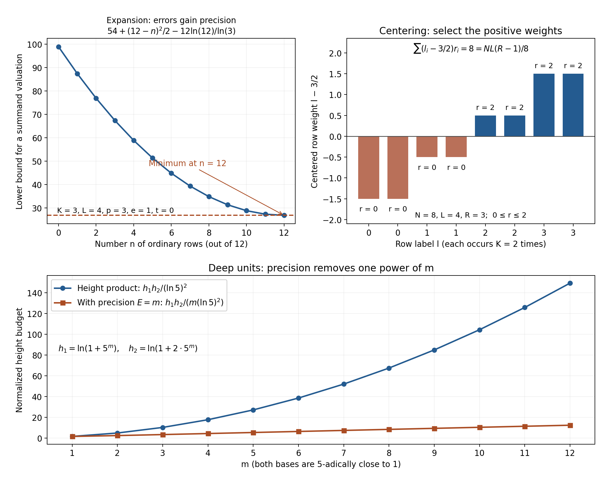
Figure 1. Left: Lemma 10.5 with \(K=3,L=4,N=12,p=3,e=1,t=0,u=0\). Under its precision hypothesis, a summand using \(n\) ordinary rows has valuation at least \(54+(12-n)^2/2-12\ln12/\ln3\); the dots are these lower bounds, not measured determinant valuations. The minimum is attained in the bound at \(n=12\). Right: Lemma 10.2 with \(K=2,L=4,N=8,R=3\). The weights are \(l_i-3/2\); selecting \(r_i=2\) on positive weights and zero on negative weights gives the exact extremum \(8=NL(R-1)/8\). Equations (10.6) and (10.14) prove these two mechanisms. Bottom: the family \(\alpha_1=1+5^m,\alpha_2=1+2\cdot5^m\) from Theorem 10.11, with \(1\le m\le12\). The curves show the calculated height budgets \(h_1h_2/(\ln5)^2\) and \(h_1h_2/(m(\ln5)^2)\), where \(h_i=h(\alpha_i)\). They illustrate the precision divisor in (10.43); the curves are height factors, while the exact difference valuation is \(m\).
4. The arithmetic determinant and a parameter theorem
For the selected columns define
\[ W=(R-1)b_2+(S-1)b_1, \qquad \beta=\frac W2 \left(\prod_{k=1}^{K-1}k!\right)^{-2/(K(K-1))}. \tag{10.15} \]Lemma 10.6 (height bound). If \(\Delta\ne0\), then
\[ v(\Delta)\le\frac{dN}{2ef\ln p} \left\{\ln N+(K-1)\ln\beta +\frac{p^tL}{2}\bigl((R-1)h(\alpha_1)+(S-1)h(\alpha_2)\bigr)\right\}. \tag{10.16} \]Proof. The polynomial
\[ P(X,Y)=\det\!\left(\binom{b_2r_j+b_1s_j}{k_i}X^{l_ir_j}Y^{l_is_j}\right) \in\mathbb Z[X,Y] \]satisfies \(\Delta=P(\alpha_1^{p^t},\alpha_2^{p^t})\). Its coefficients are integers because each binomial is evaluated at a nonnegative integer.
On \(|X|=|Y|=1\), replace the binomial basis in each \(l\)-block by \((Z-W/2)^k/k!\), again without changing the determinant. Each row has Euclidean norm at most \(\sqrt N(W/2)^k/k!\). Hadamard's inequality gives
\[ \|P\|_{\mathbb T^2}\le N^{N/2}\beta^{N(K-1)/2}. \tag{10.17} \]One can prove the inequality used here by successively subtracting orthogonal projections of each row onto the span of earlier rows. These operations preserve the determinant; the resulting perpendicular row lengths multiply to its absolute value, and each is no larger than its original row length. If the rows are dependent the determinant is zero.
Every monomial in the determinant expansion has first exponent \(\sum_i l_ir_{\pi(i)}\). Lemma 10.2 places all such exponents in an interval of length at most \(NL(R-1)/4\), and places all second exponents in an interval of length at most \(NL(S-1)/4\). Divide \(P\) by its smallest actual powers of \(X,Y\), obtaining an integer polynomial \(Q\) of these partial degrees. Multiplication by those unit powers changes neither its torus norm nor the valuation at the selected embedding.
We spell out the torus form of Liouville's inequality. For a complex polynomial of partial degrees \(a,b\), maximum modulus applied inside the unit disc, and to the reciprocal polynomial outside it, gives
\[ |Q(x,y)|\le\|Q\|_{\mathbb T^2}\max(1,|x|)^a\max(1,|y|)^b. \]Apply the one-variable argument successively. At finite places an integer polynomial satisfies the same bound without the torus factor. The weighted product formula, applied to the nonzero value, and the definition \(h(x)=d^{-1}\sum_w n_w\ln^+|x|_w\), therefore give
\[ v(Q(x,y))\le\frac d{ef\ln p} \left(\ln\|Q\|_{\mathbb T^2}+a h(x)+b h(y)\right). \]Here the selected local weight is \(ef\). A nonzero integer polynomial has torus norm at least one: any nonzero coefficient is the corresponding Fourier coefficient on the torus and has absolute value at most that norm. Thus the archimedean factor used in the product formula has nonnegative logarithm. Insert (10.17), the two degree widths, and \(h(\alpha_i^{p^t})=p^t h(\alpha_i)\). This proves (10.16). \(\square\)
Theorem 10.7 (p-adic determinant parameter theorem). Let \(K\ge3,L\ge2\), and let \(R_1,R_2,S_1,S_2\) be positive integers. Put \(R=R_1+R_2-1\), \(S=S_1+S_2-1\), \(N=KL\), and define \(\beta\) by (10.15). Suppose two residue classes \(c_1,c_2\pmod g\) satisfy
\[ \begin{aligned} \#\{\alpha_1^{p^tr}\alpha_2^{p^ts}:&\ 0\le r<R_1,\ 0\le s<S_1, \ m_1r+m_2s\equiv c_1\pmod g\}\ge L,\\ \#\{b_2r+b_1s:&\ 0\le r<R_2,\ 0\le s<S_2, \ m_1r+m_2s\equiv c_2\pmod g\}>(K-1)L. \end{aligned} \tag{10.18} \]If
\[ \begin{aligned} p^tK(L-1)\ln p>{}&(d/f+2e)\ln N+(d/f)(K-1)\ln\beta\\ &+\frac{d p^tL}{2f}\bigl((R-1)h(\alpha_1)+(S-1)h(\alpha_2)\bigr), \end{aligned} \tag{10.19} \]then
\[ v(\alpha_1^{b_1}-\alpha_2^{b_2}) <\frac{p^t}e\left(N-\frac12\right)+u. \tag{10.20} \]Proof. The two rectangles restricted to their indicated classes are sets \(E_1,E_2\). Their sum lies in the larger rectangle and class \(c_1+c_2\). Apply Lemma 10.3 with \(a_i=\alpha_i^{p^t}\). A row dependence in (10.9) would be a nonzero polynomial of the stated partial degrees vanishing on the sum set. Hence the matrix restricted to that class has row rank \(N\), and contains a nonzero minor \(\Delta\).
If (10.20) failed, Lemmas 10.5 and 10.6 would both apply. Multiply their comparison by \(2e\ln p/N\). The result is the opposite weak inequality to (10.19). This contradiction proves the theorem. \(\square\)
5. A bound with the height floor \(1/d\)
Theorem 10.8 (two p-adic logarithms). Suppose \(\alpha_1,\alpha_2\) are multiplicatively independent p-adic units, and \(b_1,b_2\) are nonzero integers. Let \(d=[\mathbb Q(\alpha_1,\alpha_2):\mathbb Q]\), and choose real \(A_i>1\) satisfying
\[ \ln A_i\ge\max\{h(\alpha_i),1/d\}. \]Define
\[ \begin{gathered} B'=\frac{|b_1|}{d\ln A_2}+\frac{|b_2|}{d\ln A_1},\\ H=\max\left\{\ln B'+\ln\ln p,\frac{10\ln p}d\right\}. \end{gathered} \tag{10.21} \]Then
\[ v(\alpha_1^{b_1}-\alpha_2^{b_2}) \le2500\,\frac{p^d-1}{(\ln p)^4}\, d^4\ln A_1\ln A_2\,H^2. \tag{10.22} \]In particular, the same inequality holds with \(132000\) in place of \(2500\).
Proof. Inverting a base when its exponent is negative makes both exponents positive, preserving the difference, heights, degree, and independence. We assume this has been done. Set
\[ G=p^d-1,\quad a_i=\frac{d\ln A_i}{\ln p},\quad z=Ga_1a_2,\quad B=\frac{dH}{\ln p},\quad k=256. \tag{10.23} \]We have \(B\ge10\), \(a_i\ge1/\ln p\), and \(z\ge d^2\ge1\). For the last assertion use \(\mathrm e^x-1\ge x^2\) for \(x\ge0\), with \(x=d\ln p\). Its derivative is \(\mathrm e^x-2x>0\), since \(\mathrm e^x\ge1+x+x^2/2>2x\), and it vanishes at \(x=0\).
Choose
\[ \begin{aligned} L&=\lfloor2B\rfloor+2,& K&=\lfloor k z L\rfloor+1,\\ R_1&=\left\lfloor\sqrt{GL a_2/a_1}\right\rfloor+1,& S_1&=\left\lfloor\sqrt{GL a_1/a_2}\right\rfloor+1,\\ R_2&=\left\lfloor\sqrt{G(K-1)L a_2/a_1}\right\rfloor+1,& S_2&=\left\lfloor\sqrt{G(K-1)L a_1/a_2}\right\rfloor+1. \end{aligned} \tag{10.24} \]Thus \(2B<L\le(11/5)B\), \(K\ge k z L\), and
\[ R_1S_1>GL\ge gL,\qquad R_2S_2>G(K-1)L\ge g(K-1)L. \tag{10.25} \]Multiplicative independence makes the products in the first rectangle distinct. Pigeonhole among the \(g\) classes gives the first condition in (10.18).
We first suppose the map \((r,s)\mapsto b_2r+b_1s\) is injective within every class of the second rectangle. Pigeonhole gives the second condition. We verify the remaining parameter inequality.
Let \(Q_K=(\prod_{j=1}^{K-1}j!)^{-2/(K(K-1))}\). Elementary integration of \(\ln x\) gives \(\ln(j!)\ge j\ln j-j\). Since \(x\ln x\) increases for \(x\ge1\),
\[ \sum_{j=1}^{K-1}j\ln j \ge\int_0^{K-1}x\ln x\,dx =\frac{(K-1)^2}2\ln(K-1)-\frac{(K-1)^2}4. \]For the first interval the integral is negative and its endpoint value is zero; for every later unit interval the increasing-function comparison applies. Consequently
\[ \ln Q_K\le-\ln(K-1)+\frac32 +\frac{\ln(K-1)-1/2}{K} \le-\ln(K-1)+2. \tag{10.26} \]The last step uses \(\ln m\le(m+1)/2\) for \(m\ge2\), obtained by differentiating from \(m=2\). Also \(K-1\ge255zL\). Formula (10.24) gives
\[ \begin{aligned} W&\le\sqrt{zL}\bigl(1+\sqrt{K-1}\bigr) \left(\frac{b_1}{a_2}+\frac{b_2}{a_1}\right),\\ \beta&\le\frac{\mathrm e^2}{2\sqrt{255}} \left(1+\frac1{\sqrt{K-1}}\right) \left(\frac{b_1}{a_2}+\frac{b_2}{a_1}\right) <\frac{b_1}{a_2}+\frac{b_2}{a_1}=B'\ln p. \end{aligned} \tag{10.27} \]Indeed \(\mathrm e<3\), \(\sqrt{255}>15\), and the parenthesis is at most two. The elementary bound \(\mathrm e<3\) follows by bounding the tail of \(\sum1/j!\) by a geometric series. Thus \(\ln\beta\le H\). Using \(d/f\le d\), \(e\le d\), \(p^t\ge1\), and the height budgets, a sufficient condition for (10.19) is
\[ K(L-1)>\frac{3d}{\ln p}\ln N +(K-1)B+L\bigl((R-1)a_1+(S-1)a_2\bigr). \tag{10.28} \]This sufficient comparison is valid even when \(\ln\beta<0\), because \(H>0\) and \(\ln\beta\le H\).
The left side minus \((K-1)B\) is at least \(k z L B\). For the height term,
\[ L\bigl((R-1)a_1+(S-1)a_2\bigr) \le2\sqrt{k}\,zL^2+2\sqrt z\,L^{3/2} <72zLB. \tag{10.29} \]To check the last strict inequality, divide by \(zLB\). The first term is at most \(32\cdot11/5=70.4\); the second is at most \(2\sqrt{(11/5)/10}<1\).
Also \(N\le257zL^2\). Since \(z\ge d^2\), we have \(d/z\le1\) and \(d\ln z/z\le1\): the latter follows from \(d\le\sqrt z\) and \(\ln z/\sqrt z\le2/\mathrm e<1\), found by differentiation. Using \(1/\ln p\le1/\ln2<2\), we obtain
\[ \frac{3d\ln N}{zLB\ln p} \le\frac{6(\ln257+1+2\ln L)}{LB} \le\frac{6(\ln257+1+2\ln20)}{200}<1. \tag{10.30} \]The middle comparison uses \(B\ge10,L\ge20\) and the decreasing function \((\ln257+1+2\ln L)/L\). For the last comparison the elementary bounds \(\ln257<6\), \(\ln20<3\) already suffice. Hence the right side of (10.28), after removing \((K-1)B\), is less than \(73zLB\); its left side is at least \(256zLB\). Theorem 10.7 applies and gives \(v(\Lambda)<2N+u\).
It remains to treat a collision in the second rectangle. Subtract the colliding labels. With \(n=\gcd(b_1,b_2)\), \(r_0=b_1/n\), \(s_0=b_2/n\), the differences are \((\ell r_0,-\ell s_0)\) for a nonzero integer \(\ell\). Put \(\sigma=\alpha_1^{r_0}\alpha_2^{-s_0}\). Its residue has an order \(q\mid g\). The class congruence gives \(q\mid\ell\), so
\[ q r_0\le R_2-1,\qquad q s_0\le S_2-1. \tag{10.31} \]If \(q\nmid n\), then \(v(\Lambda)=0\). Otherwise \(n=q p^u n'\), with \(p\nmid n'\). The prime-to-p power law, followed by the p-power laws of Lesson 9, shows
\[ v(\Lambda)=v(\sigma^n-1) \le u+v(\sigma^{q p^t}-1). \]If \(u\ge t\), the deep-domain formula gives equality with \(u-t\) in place of \(u\). If \(u<t\), raising the principal unit to further p-th powers never decreases its positive valuation, giving the displayed inequality. Independence ensures \(\sigma^{q p^t}\ne1\). Applying the weighted product formula to \(X-1\), as in Lemma 10.6, gives
\[ \begin{aligned} v(\Lambda) &\le u+\frac d{ef\ln p} \left(p^tq(r_0h(\alpha_1)+s_0h(\alpha_2))+\ln2\right)\\ &\le u+2\bigl((R_2-1)a_1+(S_2-1)a_2\bigr)+d\\ &\le u+64zL+z. \end{aligned} \tag{10.32} \]Here (10.3) bounds \(p^t/e\), (10.31) bounds the exponents, and \(d\le z\).
Finally, \(b_1\le a_2\mathrm e^H\). Since \(\ln^+a_2\le a_2\) and \(a_1\ln p\ge1\),
\[ u\le\frac{\ln b_1}{\ln p} \le\frac Bd+\frac{\ln^+a_2}{\ln p} \le B+a_1a_2\le B+z \le\frac{11}{100}zB^2. \tag{10.33} \]In the injective case,
\[ 2N+u\le\left(514\left(\frac{11}{5}\right)^2+\frac{11}{100}\right)zB^2 <2500zB^2. \]The collision bound (10.32) is at most \(14.2zB^2\), since \(L\le(11/5)B\) and \(B\ge10\). Thus both cases give (10.22), because
\[ zB^2=\frac{p^d-1}{(\ln p)^4}\,d^4\ln A_1\ln A_2\,H^2. \]This completes the proof. \(\square\)
The factor \(p^d-1\) in these parameter choices is an upper budget for the number of residue classes. It is not being asserted to equal the local residue-group order. This distinction allows the height floor \(1/d\) without inserting an additional absolute cutoff in \(H\).
6. Coprime powers and a worked example
Corollary 10.9. Let \(a>b\ge1\) be coprime positive integers, and let \(p\nmid ab\) be prime. Then
\[ v_p(a^{p-1}-b^{p-1}) \le250000\,\frac{p-1}{(\ln p)^2}\,\ln(5a)\ln(5b). \tag{10.34} \]Proof. First suppose \(b>1\). Coprimality makes the bases \(a,b\) multiplicatively independent: a prime dividing either base forces its exponent to vanish in a proposed relation. In Theorem 10.8 take \(d=1\), \(b_1=b_2=p-1\), and \(\ln A_1=\ln(5a)\), \(\ln A_2=\ln(5b)\). These exceed their rational heights and one.
For \(b=1\), choose \(c\in\{2,3,5\}\) such that \(c\ne p\) and \(a,c\) are multiplicatively independent. Such a prime always exists. Dependence of \(a\ge2\) and a prime \(c\) would force \(a=c^j\) for an integer \(j\ge1\): taking a prime valuation outside \(c\) in the relation makes the exponent of \(a\) zero unless every prime divisor is \(c\). Thus at most one of the three primes is dependent with \(a\), and excluding \(p\) removes at most one more.
Set \(\alpha_1=a/c,\alpha_2=1/c\). A relation \(\alpha_1^u\alpha_2^v=1\) is \(a^u c^{-u-v}=1\), so independence of \(a,c\) forces \(u=v=0\). Both bases are p-adic units, their common number field is \(\mathbb Q\), and \[ h(a/c)\le\ln\max\{a,c\}\le\ln(5a),\qquad h(1/c)=\ln c\le\ln5. \] Use \(\ln A_1=\ln(5a)\), \(\ln A_2=\ln5\), and again \(b_1=b_2=p-1\). The exact identity \[ \left(\frac ac\right)^{p-1} -\left(\frac1c\right)^{p-1} =c^{-(p-1)}(a^{p-1}-1) \] preserves the valuation, since \(c\ne p\).
In both cases the height choices are the stated \(\ln(5a),\ln(5b)\), and \[ B'\ln p\le\frac{2(p-1)\ln p}{\ln5}, \qquad \ln(B'\ln p)\le3\ln p<10\ln p. \] For the second inequality use \(\ln\ln p\le\ln p\), \(p-1\le p\), and \(\ln(2/\ln5)<\ln2\le\ln p\). Thus \(H=10\ln p\). Substitute it into the proved bound (10.22), and use the displayed valuation identity when \(b=1\). This proves (10.34) for every allowed prime, including \(p=2\). \(\square\)
For positive integers \(a,b\), the independent bases \(2,3\) are 5-adic units. Taking \(\ln A_1=1\), \(\ln A_2=\ln3\), Theorem 10.8 gives
\[ v_5(2^a-3^b) \le\frac{10000\ln3}{(\ln5)^4} \max\!\left\{\ln\left(\frac a{\ln3}+b\right)+\ln\ln5,10\ln5\right\}^{2}. \tag{10.35} \]If \(M=\max(a,b)\), its maximum is at most \(10\ln5+\ln(3M)\). This is an explicit constant times \((1+\ln M)^2\). For example \(2^3-3=5\), so its valuation is one; \(2^7-3=125\), so its valuation is three. These are exact illustrations of the quantity being bounded, rather than numerical evidence for the theorem.
Corollary 10.10 (all powers). For coprime \(a>b\ge1\), an odd prime \(p\nmid ab\), and \(n\ge1\),
\[ v_p(a^n-b^n) \le250000\ln(5a)\ln(5b)\frac p{(\ln p)^2}+v_p(n). \tag{10.36} \]Proof. Let \(q\mid p-1\) be the residue order of \(a/b\). If \(q\nmid n\), the valuation is zero. Otherwise write \(n=qm\). The base \((a/b)^q\) is a principal unit in \(\mathbb Q_p\), whose positive valuation is at least one and thus strictly exceeds \(1/(p-1)\). The prime-to-p and deep p-power laws proved in Lesson 9 give
\[ v_p(a^n-b^n)=v_p(a^q-b^q)+v_p(m) =v_p(a^{p-1}-b^{p-1})+v_p(n). \]Here \(p\nmid q\) and \(p\nmid(p-1)/q\). Apply Corollary 10.9 and \(p-1\le p\). \(\square\)
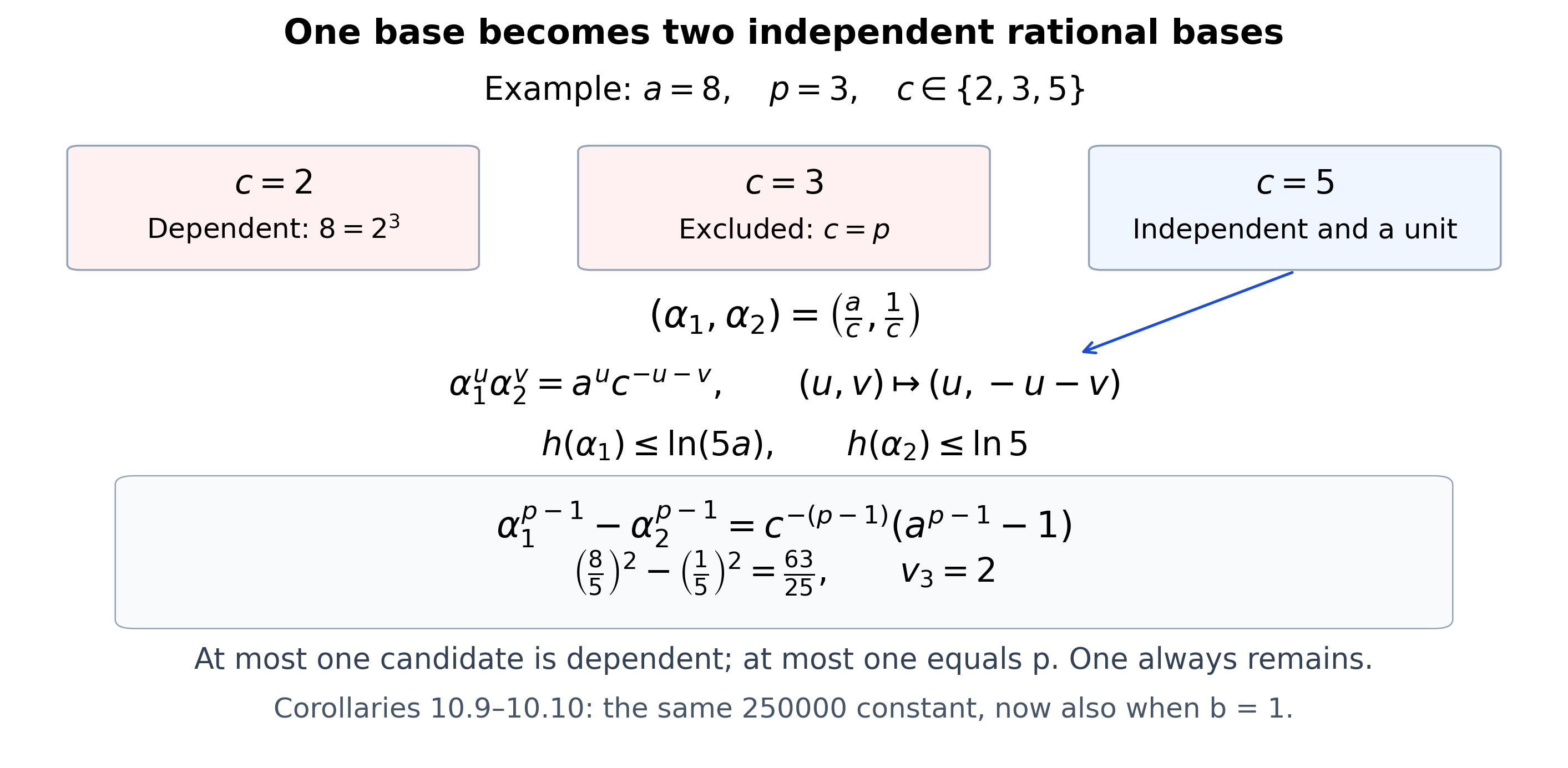
Figure 10.1b. Choose \(c\in\{2,3,5\}\) with \(c\ne p\) and independent of \(a\). At most one candidate is removed by dependence and at most one by the prime \(p\). The invertible exponent change \((u,v)\mapsto(u,-u-v)\) proves that \(a/c,1/c\) are independent. The lower row gives the exact unit-factor identity and the height choices \(\ln A_1=\ln(5a),\ln A_2=\ln5\). The example \(a=8,p=3\) removes \(c=2\) by dependence and \(c=3\) by the unit condition, leaving \(c=5\); both differences have valuation two. The complete argument is Corollaries 10.9–10.10, and Solution 30 verifies the examples and the height cutoff. Human-source context: the determinant estimate from Bugeaud's freely accessible 1999 paper, cited below; the auxiliary-prime embedding here is proved explicitly from Theorem 10.8. Figure program.
7. A deep-unit refinement
The precision of the first base can improve the height factor. We state the coefficient and convergence conditions explicitly.
Theorem 10.11 (an E-parameter estimate). Let \(\alpha_1,\alpha_2\) be multiplicatively independent nonzero rationals with \(v_p(\alpha_i)=0\). Put \(g=p-1\), and suppose
\[ v_p(\alpha_1^g-1)\ge E>\frac1{p-1}. \tag{10.37} \]If \(p=2\), require also \(v_2(\alpha_2-1)\ge2\). Let \(b_1,b_2\) be nonzero integers, \(u=v_p(\gcd(b_1,b_2))\), and require \(p\nmid b_2/p^u\). Choose
\[ \begin{gathered} \ln A_i\ge\max\{h(\alpha_i),E\ln p\},\\ B'=\frac{|b_1|}{\ln A_2}+\frac{|b_2|}{\ln A_1},\qquad H_E=\max\{\ln B'+\ln(E\ln p),10E\ln p\}. \end{gathered} \tag{10.38} \]Then
\[ v_p(\alpha_1^{b_1}-\alpha_2^{b_2}) \le1300\,\frac{p-1}{E^3(\ln p)^4}\, \ln A_1\ln A_2\,H_E^2. \tag{10.39} \]Consequently this inequality also holds with \(88000\) in place of \(1300\).
Proof. Invert bases with negative exponents as before. Inversion preserves the precision conditions, because the denominators introduced are units. Decompose \(\alpha_i=\eta^{m_i}\epsilon_i\) as in (10.1), now in \(\mathbb Q_p\). Since \(p\nmid g\), the prime-to-p power law gives \(v(\epsilon_1-1)=v(\alpha_1^g-1)\ge E\). Both principal units are in the exponential domain. For odd \(p\) their positive integer valuations are at least one, greater than \(1/(p-1)\); for \(p=2\), (10.37) and the second-base condition give valuations at least two.
If the original difference has valuation zero, the conclusion is immediate. Otherwise its residue factors agree, so it has the valuation of \(\epsilon_1^{b_1}-\epsilon_2^{b_2}\). For \(b_i'=b_i/p^u\), the deep p-power law gives
\[ \delta=\epsilon_1^{b_1'}-\epsilon_2^{b_2'}, \qquad v(\delta)=v(\alpha_1^{b_1}-\alpha_2^{b_2})-u. \]The matrix (10.9) is used with exponent multiplier one. In Lemma 10.5 take \(\omega=\log\epsilon_1\), so \(v(\omega)\ge E\). The assumed unit denominator \(b_2'\) gives \(z_j=r_j+(b_1'/b_2')s_j\in\mathbb Z_p\). Formula (10.11) holds with multiplier one and no root of unity in \(\delta\). The coefficient of its error part remains integral whenever \(v(\delta)>1/(p-1)\).
We give the resulting comparison, keeping the scale change visible. If \(v(\delta)\ge E(N-1/2)\), the alternant and factorial estimates in (10.13) give
\[ \begin{aligned} v(A)&\ge E\left(\frac{n(n-1)}2-\sum_{i\in I}k_i\right)-\frac{n\ln n}{\ln p},\\ v(B)&\ge-\frac{\sum_{i\notin I}k_i}{p-1} \ge-E\sum_{i\notin I}k_i. \end{aligned} \]The positive coefficient \(E-1/(p-1)\) is what permits replacement of the Taylor-order sum by \(n(n-1)/2\). Formula (10.14) then gives
\[ v(\Delta)\ge\frac{ENK(L-1)}2-\frac{N\ln N}{\ln p}. \]The polynomial height proof of Lemma 10.6 has \(d=e=f=1\) and exponent multiplier one. Thus a sufficient parameter inequality is
\[ EK(L-1)\ln p> 3\ln N+(K-1)\ln\beta +\frac L2\bigl((R-1)h(\alpha_1)+(S-1)h(\alpha_2)\bigr). \tag{10.40} \]Under the two cardinality conditions (10.18), the zero lemma and these two bounds prove \(v(\Lambda)<E(N-1/2)+u\).
Use (10.24) with
\[ G=p-1,\qquad a_i=\frac{\ln A_i}{E\ln p},\qquad z=Ga_1a_2,\qquad B=\frac{H_E}{E\ln p},\qquad k=256. \tag{10.41} \]Here \(a_i\ge1\), \(z\ge G\ge1\), and \(B\ge10\). The cardinalities, factorial estimate and height comparison (10.25)–(10.29) apply unchanged, with \(B' E\ln p=b_1/a_2+b_2/a_1\). In particular \(\ln\beta\le H_E\), and the height contribution after division by \(E\ln p\) is less than \(72zLB\).
We check the remaining logarithmic contribution. From \(E>1/G\) and \(z\ge G\),
\[ \frac1{Ez\ln p}<\frac1{\ln p}<2, \qquad \frac{\ln z}{Ez\ln p}\le1. \]For the second bound, at \(p=2,3\) use \(1/(E\ln p)<2\) and \(\ln z/z\le1/\mathrm e\). For \(p\ge5\), the function \(\ln z/z\) decreases on \(z\ge G\ge4\), giving a bound \(\ln G/\ln p<1\). With \(N\le257zL^2\), therefore,
\[ \frac{3\ln N}{EzLB\ln p} \le\frac{6(\ln257+1+2\ln L)}{LB}<1. \]The left side of the sufficient parameter inequality, after removing \((K-1)B\), is at least \(256zLB\), while its remaining right side is less than \(73zLB\). This verifies (10.40) in the injective case.
In the collision case, take \(q,r_0,s_0\) as in (10.31). If \(q\nmid n=\gcd(b_1,b_2)\), the valuation is zero. Otherwise \(\sigma^q\), with \(\sigma=\alpha_1^{r_0}\alpha_2^{-s_0}\), is a deep principal unit: its residue root has disappeared, and its two principal factors were already deep. Hence \(v(\Lambda)=u+v(\sigma^q-1)\). The one-place polynomial bound for \(X-1\) gives
\[ \begin{aligned} v(\Lambda) &\le u+\frac{q(r_0h(\alpha_1)+s_0h(\alpha_2))+\ln2}{\ln p}\\ &\le u+E\bigl((R_2-1)a_1+(S_2-1)a_2\bigr)+1\\ &\le u+32EzL+1\le u+Ez(32L+1). \end{aligned} \tag{10.42} \]Here \(Ez>EG>1\). Finally \(b_1\le a_2\mathrm e^{H_E}\), so
\[ u\le EB+\frac{\ln^+a_2}{\ln p} \le EB+2Ez\le\frac{12}{100}EzB^2. \]The middle bound uses \(\ln^+a_2\le a_2\), \(EGa_1>1\), and \(1/\ln p<2\). In the injective case,
\[ EN+u\le \left(257\left(\frac{11}{5}\right)^2+\frac{12}{100}\right)EzB^2 =1244EzB^2<1300EzB^2. \]The collision bound is at most \(7.17EzB^2\). Substituting (10.41) into \(EzB^2\) proves (10.39). \(\square\)
The coefficient condition singles out the first base whose logarithm supplies the precision \(E\). Interchanging bases is permissible only if the precision and second-base convergence hypotheses are checked for the newly ordered pair. At \(p=2\), a unit such as three has \(v_2(3-1)=1\), on the exponential boundary; its positivity alone does not provide the deep-unit substitution used in this proof.
For a concrete family take
\[ \alpha_1=1+5^m,\qquad \alpha_2=1+2\cdot5^m,\qquad E=m,\qquad m\ge1. \]The two integers are coprime, because twice the first minus the second is one. They exceed one, so they are multiplicatively independent. Their fourth powers have distance valuation \(m\) from one, by the prime-to-five power law. Both height budgets may be their actual logarithms. For \(b_1=b_2=1\), \(H_E=10m\ln5\) and the exact difference valuation is \(m\). The bound (10.39) is
\[ v_5(\alpha_1-\alpha_2) \le520000\, \frac{\ln(1+5^m)\ln(1+2\cdot5^m)}{m(\ln5)^2}. \tag{10.43} \]The height factor is linear in \(m\), bounded explicitly by \((m\ln5+\ln2)(m\ln5+\ln3)/(m(\ln5)^2)\). Without the precision divisor, the product of these heights is quadratic in \(m\).
8. Saturated bases and Kummer degree
We now allow an arbitrary number of bases. A root which already belongs to the number field should be incorporated into the bases before taking an auxiliary extension. The following construction does this and proves the resulting extension degree.
Let \(K\) be a number field of degree \(d\), embedded in \(\mathbb C\). Let \(q\) be a prime, and assume that \(K\) contains all the q-th roots of unity. For \(n\ge1\) and multiplicatively independent \(\alpha_1,\ldots,\alpha_n\in K^*\), define
\[ \begin{aligned} M_q(\boldsymbol\alpha)=\{\boldsymbol v\in\mathbb Z[1/q]^n:\ &\text{for some }T=q^t, \ T\boldsymbol v\in\mathbb Z^n,\\ &\alpha_1^{Tv_1}\cdots\alpha_n^{Tv_n}=\beta^T \text{ for some }\beta\in K^*\}. \end{aligned} \tag{10.44} \]No choice of complex logarithms is involved in this definition.
The complete finite-height count in Heights of algebraic numbers, Theorem 2.6, bounds the number of algebraic numbers of degree at most \(d\) and height at most \(H\ge0\) by
\[ \mathcal N(d,H)=d^2\bigl(2^{d+1}\mathrm e^{dH}+1\bigr)^{d+1}. \tag{10.45} \]We use its polynomial coefficient proof and the height arithmetic of Proposition 2.5 in that earlier lesson.
Lemma 10.12 (finite saturation). The set \(M=M_q(\boldsymbol\alpha)\) is an additive subgroup of \(\mathbb Q^n\), contains \(\mathbb Z^n\), and has finite index over it. More precisely,
\[ [M:\mathbb Z^n]\le\mathcal N\left(d,\sum_{j=1}^n h(\alpha_j)\right). \tag{10.46} \]This index is a power of \(q\). The group \(M\) has a basis of \(n\) rational vectors over \(\mathbb Z\).
Proof. Powers \(T\) in (10.44) can be enlarged to a common power of \(q\). Multiplying or dividing the corresponding \(\beta\)'s proves closure under addition and subtraction. Integral vectors belong to \(M\) with \(T=1\).
Every coset modulo \(\mathbb Z^n\) has a unique representative \(\boldsymbol v\) with \(0\le v_j<1\). Choose one associated \(\beta\) from (10.44). The product inequality and power identity in Heights of algebraic numbers, Proposition 2.5, give
\[ T h(\beta)=h\left(\prod_j\alpha_j^{Tv_j}\right) \le T\sum_j v_jh(\alpha_j)\le T\sum_j h(\alpha_j). \]Distinct representatives give distinct chosen \(\beta\)'s. Indeed, if two choices were equal, raise their defining equations to a common power \(T\). Their quotient would give \(\prod_j\alpha_j^{T(v_j-w_j)}=1\). Independence forces every \(v_j=w_j\). The earlier finite-height count (10.45) therefore bounds the number of cosets as asserted.
There are finitely many representatives, and each has a denominator which is a power of \(q\). Choose a common denominator \(q^a\). Then \(\mathbb Z^n\subset M\subset q^{-a}\mathbb Z^n\). The finite group \(M/\mathbb Z^n\) is a subgroup of \((q^{-a}\mathbb Z/\mathbb Z)^n\), so its order is a power of \(q\).
For completeness, a subgroup \(L\subset\mathbb Z^n\) containing \(m\mathbb Z^n\), with \(m>0\), has an integral basis of size \(n\). Prove this by induction. Its first-coordinate image is \(c\mathbb Z\) for some \(c>0\): take the least positive first coordinate and apply integer division. Choose \(\boldsymbol x\in L\) with first coordinate \(c\). The kernel of that projection contains \(m\mathbb Z^{n-1}\), so has an \((n-1)\)-element basis by induction. Any element of \(L\) becomes an element of the kernel after subtracting the appropriate integer multiple of \(\boldsymbol x\). These \(n\) vectors are independent and span \(L\). Apply this to \(L=q^aM\) and divide its basis by \(q^a\). \(\square\)
Lemma 10.13 (the maximal q-primary root). The q-primary roots of unity in \(K\) form a finite cyclic group. If \(\alpha_0\) generates it and has order \(q^u\), then \(u\ge1\), and \(\alpha_0^a\) is not a q-th power in \(K\) when \(q\nmid a\).
Proof. Roots of unity have height zero, by the height power identity. Finiteness follows from (10.45) with \(H=0\). The finite-subgroup argument of Section 1 applies over any field: its root count and the existence of an element of maximal exponent prove cyclicity. The assumption that q-th roots are in \(K\) gives \(u\ge1\). If \(\beta^q=\alpha_0^a\) with \(q\nmid a\), then \(\beta^{q^{u+1}}=1\), while its q-th power has order \(q^u\). Thus \(\beta\) has order \(q^{u+1}\), contradicting maximality of \(u\). \(\square\)
Fix such a generator \(\alpha_0\).
Choose a basis \(\boldsymbol v_1,\ldots,\boldsymbol v_n\) of \(M\). By (10.44), after choosing a common power \(T=q^t\), there are \(\theta_i\in K^*\) with
\[ \theta_i^T=\prod_{j=1}^n\alpha_j^{T v_{ji}}, \qquad v_{ji}=(\boldsymbol v_i)_j. \tag{10.47} \]Theorem 10.14 (the saturated Kummer condition). The classes of \(\alpha_0,\theta_1,\ldots,\theta_n\) in \(K^*/(K^*)^q\) are linearly independent over \(\mathbb F_q\). Consequently
\[ [K(\alpha_0^{1/q},\theta_1^{1/q},\ldots,\theta_n^{1/q}):K] =q^{n+1}. \tag{10.48} \]Proof. Suppose \(\alpha_0^{a_0}\prod_i\theta_i^{a_i}=\beta^q\), with integers \(a_i\) and \(\beta\in K^*\). Enlarge \(T\) in (10.47) until it is divisible by the order of \(\alpha_0\). Raising the relation to \(T\) shows that
\[ \boldsymbol w=\frac1q\sum_i a_i\boldsymbol v_i\in M: \quad \prod_j\alpha_j^{qT w_j}=\beta^{qT}. \]Uniqueness of integral coordinates in the basis of \(M\) forces \(q\mid a_i\) for \(1\le i\le n\). Dividing out the corresponding q-th powers, we find that \(\alpha_0^{a_0}\) is a q-th power in \(K\). If \(q\nmid a_0\), its q-th root would have order \(q^{u+1}\), contradicting the choice of \(\alpha_0\). Thus \(q\mid a_0\) as well. This proves independence of all the classes.
We prove the degree consequence directly. More generally, let \(c_1,\ldots,c_r\in K^*\) have independent classes modulo q-th powers, and choose roots \(\rho_i^q=c_i\). The field \(L=K(\rho_1,\ldots,\rho_r)\) splits the separable polynomials \(X^q-c_i\), since all q-th roots of unity are already in \(K\). Fix a primitive q-th root \(\zeta\). Every \(K\)-automorphism acts by \(\rho_i\mapsto\zeta^{t_i}\rho_i\), giving an injective group homomorphism
\[ \operatorname{Aut}_K(L)\longrightarrow\mathbb F_q^r. \]Its image is a vector subspace. If it were proper, Gaussian elimination would give a nonzero vector \(\boldsymbol a\in\mathbb F_q^r\) annihilating it. Choose integer representatives \(0\le a_i<q\). The element \(\prod_i\rho_i^{a_i}\) would then be fixed by every automorphism and would belong to \(K\). Its q-th power is \(\prod_i c_i^{a_i}\), contradicting the independence of the classes.
Here the fixed-element assertion and the automorphism count need only elementary separability. An embedding of an intermediate field extends across each algebraic generator by choosing a root of the transported minimal polynomial. In characteristic zero these roots are distinct, so the number of embeddings of \(L\) equals the product of the successive degrees, namely \([L:K]\). Since \(L\) is a splitting field, every such embedding has image \(L\). If an element outside \(K\) were fixed, choose a different root of its separable minimal polynomial and extend that embedding to \(L\); the resulting automorphism would move it. Thus the fixed elements are precisely \(K\).
The automorphism image is therefore all of \(\mathbb F_q^r\), and \([L:K]=q^r\). Apply this with \(r=n+1\) and the already proved independent classes. \(\square\)
Lemma 10.15 (the residue index does not depend on the saturated basis). Suppose \(q\ne p\), a prime of \(K\) above \(p\) is fixed, and every \(\alpha_j\) is a unit there. The group \(\langle\alpha_0,\theta_1,\ldots,\theta_n\rangle\subset K^*\) is independent of the basis and of the root choices in (10.47). Its generators are p-adic units. If the residue field has size \(p^f\), the integer
\[ \delta_q(\boldsymbol\alpha)= \frac{p^f-1}{|\langle\overline{\alpha_0},\overline{\theta_1}, \ldots,\overline{\theta_n}\rangle|} \tag{10.49} \]is consequently well defined.
Proof. Replacing a root choice in (10.47) multiplies \(\theta_i\) by a q-primary root of unity in \(K\), hence by a power of \(\alpha_0\). For a change of basis write \(\boldsymbol v_i'=\sum_j c_{ji}\boldsymbol v_j\), with the integer matrix \(C\) invertible over \(\mathbb Z\). Raising to a common power \(T=q^t\) shows that \(\theta_i'/\prod_j\theta_j^{c_{ji}}\) is again a q-primary root of unity. The new group is contained in the old one. Applying the inverse integral matrix gives the reverse inclusion.
Taking the valuation in (10.47) gives \(v(\theta_i)=0\); roots of unity are units too. Reduction is therefore defined. Its image is a subgroup of the cyclic group of order \(p^f-1\) proved in Section 1, so its order divides \(p^f-1\), and the quotient in (10.49) is an integer. Basis independence proves the final assertion. \(\square\)
For example, take \(K=\mathbb Q\), \(q=2\), \(\alpha_1=4\), and \(\alpha_2=9\). Prime valuations show that \(M_2(4,9)=\tfrac12\mathbb Z^2\). A saturated basis gives \(\theta_1=2,\theta_2=3\), and \(\alpha_0=-1\). Theorem 10.14 proves
\[ [\mathbb Q(\sqrt{-1},\sqrt2,\sqrt3):\mathbb Q]=8. \]Starting with \(4,9\) would instead leave both classes trivial modulo squares. Saturation exposes the arithmetic independence needed for the auxiliary extension.
9. Counting heights and bounding saturation
The index in (10.46) is finite, but its bound uses the sum of the heights inside an exponential. A sharper count gives a product of heights and a small power of the field degree. This is the arithmetic input for reducing a form with many logarithms to independent bases.
Write \(\mathcal H(\gamma)=\exp h(\gamma)\) for multiplicative height. Let \(K\) have degree \(d\). The number field containing a scalar \(\theta\) below can be larger than \(K\).
Lemma 10.16 (a count at one archimedean place). Fix an archimedean place of \(K\), represented by \(\sigma:K\to\mathbb C\), and put \(f=1\) for a real place and \(f=2\) for a complex place. Fix \(\phi\ne0\) algebraic and a number field \(L\supset K(\phi)\), of degree \(\ell\). Use the product-formula absolute values of \(L\), and set
\[ \begin{aligned} \Phi_v&=\prod_{w\mid v}|\phi|_w^{1/\ell},& \Phi_{\widehat v}&=\prod_{w\nmid v}|\phi|_w^{1/\ell},\\ A_v(a)&=\prod_{w\mid v}\max\{|\phi|_w,|a|_w\}^{1/\ell},& A_{\widehat v}(a)&=\prod_{w\nmid v}\max\{|\phi|_w,|a|_w\}^{1/\ell}. \end{aligned} \]Thus \(\Phi_v\Phi_{\widehat v}=1\), and \(A_v(a)A_{\widehat v}(a)=\mathcal H(a/\phi)\). If \(X,Y\ge1\), \(N\ge2\), and \(u=N^{1/(N-1)}\), then
\[ \#\{a\in K:A_v(a)\le X\Phi_v, \ A_{\widehat v}(a)\le Y\Phi_{\widehat v}\} \le (N-1)\left(1+(uXY^2)^{d/f}\right)^f. \tag{10.50} \]Proof. Finiteness follows from the earlier finite-height count: the numbers \(a/\phi\) lie in \(L\), have degree at most \(\ell\), and have height at most \(\ln(XY)\). The identity for \(A_vA_{\widehat v}\) follows by factoring \(|\phi|_w\) from each maximum and applying the product formula to \(\phi\).
The first local inequality implies \(|\sigma a|\le R\), where \(R=(X\Phi_v)^{d/f}\). This follows because the sum of archimedean weights above \(v\) is \(f\ell/d\). Indeed, each embedding of \(K\) has \([L:K]\) extensions; conjugate complex embeddings contribute weight two, and real embeddings contribute weight one.
Put \(r=(uY^2\Phi_{\widehat v})^{-d/f}\). Draw around each \(\sigma a\) a ball of radius \(r\) in \(\mathbb R^f\). These balls lie in the ball of radius \(R+r\). We show that no point is in the interiors of \(N\) of them.
Otherwise there are distinct \(a_1,\ldots,a_N\) whose images lie in a ball of radius strictly less than \(r\), with centre \(z\). Put \(Q=N(N-1)/2\), and let \(\Delta=\prod_{i<j}(a_j-a_i)\ne0\). Translating the Vandermonde rows replaces \((\sigma a_i)^k\) by \((\sigma a_i-z)^k\) without changing the determinant. Factoring the radius from its rows and using Hadamard's inequality gives \(|\sigma\Delta|<N^{N/2}r^Q=u^Qr^Q\). Here Hadamard's inequality follows by orthogonalizing the columns: this preserves the determinant and weakly decreases their norms, while the determinant of the orthogonal columns has absolute value the product of those norms.
At a finite place \(w\nmid v\), expand the determinant into its permutation monomials. Every monomial has total degree \(Q\) and degree at most \(N-1\) in each \(a_i\). With \(\lambda=|\phi|_w\), its absolute value is at most
\[ \lambda^{-Q}\prod_i\max\{\lambda,|a_i|_w\}^{N-1}. \]The ultrametric inequality gives the same bound for \(\Delta\). At an archimedean embedding \(\tau\) outside \(v\), apply Hadamard to the powers of \(\tau a_i/\tau\phi\). Each column has norm at most \(\sqrt N\max\{1,|\tau a_i/\tau\phi|\}^{N-1}\), so the same bound has the extra factor \(N^{f_wN/2}\), where \(f_w=1\) or two is its archimedean weight.
Crucially, the sum of these unselected archimedean weights is exactly \(\ell(d-f)/d\). Multiplying their bounds and the finite-place bounds gives
\[ \prod_{w\nmid v}|\Delta|_w \le u^{\ell Q(d-f)/d} Y^{2\ell Q}\Phi_{\widehat v}^{\ell Q}. \]The selected place contributes strictly less than \((ur)^{f\ell Q/d}\). The full product is therefore strictly less than \((r^{f/d}uY^2\Phi_{\widehat v})^{\ell Q}=1\), contrary to the product formula. This proves the asserted multiplicity bound for the balls.
Integrate their indicator functions. Their sum is at most \(N-1\) outside their boundaries, which have volume zero. Scaling a ball's volume by its radius gives \(M r^f\le(N-1)(R+r)^f\) for the number \(M\) of centres. Since \(R/r=(uXY^2)^{d/f}\), this is (10.50). \(\square\)
We need a uniform choice of \(N\). For \(d\ge2\), take
\[ m=\lfloor d\ln d\rfloor,\qquad N=m+1,\qquad u=N^{1/m},\qquad u^d<8. \tag{10.51} \]Here is a proof of the last inequality for every degree. For \(d=2,3\), the choices are \(N=2,4\), giving \(u^d=4\) in both cases. For \(d\ge4\), put \(x=d\ln d>4\). Then \(m\ge3x/4\), \(N\le5x/4\), and
\[ \frac{d\ln N}{m} \le\frac43\left(1+\frac{\ln\ln d}{\ln d} +\frac{\ln(5/4)}{\ln d}\right) <\frac43\left(1+\frac38+\frac16\right)=\frac{37}{18}<\ln8. \]The first fraction is at most \(1/\mathrm e<3/8\), by differentiating \(\ln t/t\). The second is less than \(1/6\), since \((5/4)^6<4\). Finally \(\ln2=2\sum_{j\ge0}(1/3)^{2j+1}/(2j+1)>56/81\), which proves \(\ln8>37/18\). This series follows by integrating the geometric series on \([0,1/3]\). The elementary bounds \(8/3<\mathrm e<3\) follow directly from its exponential series. They give \(1/2<\ln2<1\) and \(1<\ln3<4/3\); for the last upper bound, use \((8/3)^4>3^3\). These also verify the two small choices of \(N\).
Theorem 10.17 (uniform twisted height count). Let \(\theta\ne0\) be algebraic and \(H\ge1\). The following bounds hold:
\[ \begin{aligned} \#\{a\in K:\mathcal H(\theta a)\le H\} &\le68d\ln d\,H^{2d} &&(d\ge2),\\ &\le31d\ln d\,H^{2d} &&(d\ge2,\ \theta\in K),\\ &\le17H^2 &&(d=1). \end{aligned} \tag{10.52} \]Proof. Apply Lemma 10.16 with \(\phi=1/\theta\). Both ratios \(A_v/\Phi_v\) and \(A_{\widehat v}/\Phi_{\widehat v}\) are at least one, and their product is \(\mathcal H(\theta a)\). Divide the first ratio into bands \(2^{(i-1)/d}\le A_v/\Phi_v<2^{i/d}\). There are at most \(I=1+\lfloor d\ln H/\ln2\rfloor\) bands. Within band \(i\), set \(X_i=2^{i/d}\), \(Y_i=2^{-(i-1)/d}H\). Then \(X_iY_i^2=2^{(2-i)/d}H^2\).
Let \(M(H)\) denote the count. Summing (10.50), using \(I\le H^d\), \(\sum_{i\ge1}2^{2-i}=4\), and \(\sum_{i\ge1}2^{(2-i)/2}=2/(\sqrt2-1)\), gives
\[ \begin{aligned} M(H)&\le m(1+4u^d)H^{2d} &&(f=1),\\ M(H)&\le m\left[ \left(1+\frac{4u^{d/2}}{\sqrt2-1}\right)H^d +4u^dH^{2d}\right] &&(f=2). \end{aligned} \tag{10.53} \]To see \(I\le H^d\), put \(t=H^d\); if \(k=\lfloor\log_2t\rfloor\), then \(k+1\le2^k\le t\). With (10.51), the first coefficient is less than 33, and the two coefficients in the second line are less than 31 and 32: use \(\sqrt8<3\) and \(1/(\sqrt2-1)=1+\sqrt2<5/2\). Since \(m\le d\ln d\), both imply the first assertion of (10.52). For \(d=1\), take \(N=2,u=2\) instead. The first line yields \(M(H)\le H+8H^2\le9H^2<17H^2\).
If \(\theta\in K\), multiplication by \(\theta\) is a bijection, so reduce to \(\theta=1\). The set contains \(0,1,-1\). All other elements pair as \(a,a^{-1}\), with equal heights, and at least one member of each pair satisfies \(|\sigma a|\le1\). Consequently a subset of cardinality \((M(H)+3)/2\) satisfies the inequalities of Lemma 10.16 with \(X=1,Y=H,\phi=1\). At a complex place this gives \(M(H)\le2m(1+u^{d/2}H^d)^2-3\le30d\ln d\,H^{2d}\); at a real place it gives \(M(H)\le2m(1+u^dH^{2d})-3\le18d\ln d\,H^{2d}\). These prove the second assertion. \(\square\)
Theorem 10.18 (the full saturation index). For independent \(\alpha_1,\ldots,\alpha_n\in K^*\), define
\[ M_K(\boldsymbol\alpha)= \{\boldsymbol v\in\mathbb Q^n: T\boldsymbol v\in\mathbb Z^n, \ \prod_j\alpha_j^{Tv_j}=\beta^T \text{ for some }T\ge1,\ \beta\in K^*\}. \tag{10.54} \]Let \(w_K\) be the number of roots of unity in \(K\). This is a lattice containing \(\mathbb Z^n\), and
\[ w_K[M_K:\mathbb Z^n] \le C_d\frac{n!\mathrm e^n}{n^n}\prod_jh(\alpha_j), \qquad C_d=\begin{cases}58d^{n+1}\ln d,&d\ge2,\\17,&d=1. \end{cases} \tag{10.55} \]Proof. Common integer powers prove that \(M_K\) is a subgroup. The coset argument of Lemma 10.12 applies with arbitrary positive integers \(T\): distinct representatives in \([0,1)^n\) give distinct elements of \(K\) of height at most \(\sum h(\alpha_j)\). Thus its index \(J\) is finite. A common denominator puts it between \(\mathbb Z^n\) and \(T^{-1}\mathbb Z^n\); the integral basis induction there proves it is a lattice. Its fundamental volume is \(1/J\), since the unit-volume fundamental domain of \(\mathbb Z^n\) contains \(J\) fundamental domains of \(M_K\).
The group of all roots of unity in \(K\) is finite by (10.45) with height zero, and the finite-subgroup argument of Section 1 makes it cyclic. Each \(h_j=h(\alpha_j)\) is positive: otherwise all powers of \(\alpha_j\) have height zero and lie in \(K\), so the same finite-height count would make two powers equal, contradicting independence.
For \(H>1\), the open diamond
\[ S=\{\boldsymbol x:\sum_jh_j|x_j|<\ln H\} \quad\text{has volume}\quad V=\frac{2^n(\ln H)^n}{n!\prod_jh_j}. \tag{10.56} \]In each orthant, scale the coordinates by \(h_j\) and integrate the simplex \(\sum y_j<\ln H\); induction by its last coordinate gives volume \((\ln H)^n/n!\). This proves the volume formula.
Average the count \(\sum_{\boldsymbol v\in M_K}1_S(\boldsymbol t+\boldsymbol v)\) over a fundamental domain. Translating its integrals tiles \(\mathbb R^n\), so the integral equals \(V\) and its average equals \(JV\). Some coset therefore has at least \(JV\) points in \(S\). There are only finitely many in the bounded diamond. Since \(S\) is open, perturb the translating vector to a rational vector while retaining this finite set of points. Denote the resulting rational points by \(P_0,\ldots,P_s\); their differences still lie in \(M_K\), and \(s+1\ge JV\).
Choose determinations \(\theta_i=\prod_j\alpha_j^{(P_i)_j}\). They are algebraic because the coordinates are rational. The definition of \(M_K\) gives \(\theta_i/\theta_0=\mu_i\beta_i\) for \(\beta_i\in K\) and roots of unity \(\mu_i\) in an algebraic closure. The height power and product identities give \(h(\theta_0\beta_i)=h(\theta_i)<\ln H\). Multiplying by a root of unity preserves height: raise to its order and use the power identity.
The \(\beta_i\) are distinct modulo roots of unity in \(K\). If a quotient were a root of unity, then so would \(\theta_i/\theta_j\); raising to a common denominator and then to its order would contradict independence of the \(\alpha_j\). Consequently their \(w_K\) root-of-unity multiples give \(w_K(s+1)\) distinct elements of \(K\) counted by Theorem 10.17 with twist \(\theta_0\). Hence \(w_KJV\le M(H)\).
Take \(H=\exp(n/(2d))\). At a complex place, (10.53) divided by \(\exp(n)\) is less than \(d\ln d(31/\sqrt{\mathrm e}+32)<58d\ln d\), since \(\sqrt{\mathrm e}>3/2\). At a real place the coefficient is less than \(33d\ln d\). Substitute (10.56) to obtain (10.55). For \(d=1\), the bound \(17H^2\) gives exactly its stated constant 17. \(\square\)
In particular, since \(w_K\ge1\) and the index is at least one,
\[ \prod_jh(\alpha_j)\ge \frac{w_K}{C_d}\frac{n^n}{n!\mathrm e^n}. \tag{10.57} \]Corollary 10.19 (the q-primary part). The lattice of Section 8 is exactly \(M_q=M_K\cap\mathbb Z[1/q]^n\). Therefore (10.55) also bounds \(w_K[M_q:\mathbb Z^n]\).
Proof. Only the reverse inclusion needs proof. For a vector in the intersection, write a power realizing (10.54) as \(T=q^a m\) with \(q\nmid m\). Since its coordinates have q-power denominators, \(q^a\boldsymbol v\) is integral. Put \(\gamma=\prod_j\alpha_j^{q^av_j}\). The defining equation says \(\gamma^m=\beta^{q^am}\), so \(\zeta=\gamma/\beta^{q^a}\in K\) has order dividing \(m\). Raising to \(q^a\) is a bijection on this finite cyclic group, by Bezout's identity for \(q^a,m\). Choose \(\eta\in\langle\zeta\rangle\) with \(\eta^{q^a}=\zeta\). Then \(\gamma=(\beta\eta)^{q^a}\), which realizes (10.44). The inclusion of finite quotients gives the index inequality. \(\square\)
Corollary 10.20 (a primitive circuit relation). Suppose \(\alpha_0,\ldots,\alpha_n\in K^*\) are dependent but every \(n\) of them are independent. There are nonzero integers \(b_i\) with \(\prod_i\alpha_i^{b_i}=1\) and
\[ |b_i|\le C_d\frac{n!\mathrm e^n}{n^n} \prod_{j\ne i}h(\alpha_j)\qquad(0\le i\le n), \tag{10.58} \]where \(C_d\) is the degree factor in (10.55).
Proof. The integer vectors whose products are roots of unity have rational rank one. Two nonproportional such vectors could eliminate a coordinate, producing a nonzero torsion relation on only \(n\) bases; raising to the torsion order contradicts their independence. Divide any nonzero relation vector by its coordinate gcd to obtain a primitive vector \(\boldsymbol r\). Its product is still a root of unity, since a power of that product is one. All \(r_i\ne0\), and every integer vector in this rational line is an integer multiple of \(\boldsymbol r\), by Bezout's identity for its coordinate gcd.
The vector \((r_1/r_0,\ldots,r_n/r_0)\) belongs to \(M_K(\alpha_1,\ldots,\alpha_n)\): take \(T=|r_0|w_K\) and \(\beta=\alpha_0^{-1}\) in (10.54). The root of unity in the relation disappears upon raising to \(T/r_0\). Its order modulo \(\mathbb Z^n\) is exactly \(|r_0|\), again by Bezout's identity for the coordinate gcd. Thus \(|r_0|\le[M_K:\mathbb Z^n]\). Set \(b_i=w_Kr_i\); their product is one, and (10.55) proves the bound for \(b_0\). Apply the same argument after omitting each other coordinate. The vector \(\boldsymbol b\) is the same throughout, so all the bounds hold simultaneously. \(\square\)
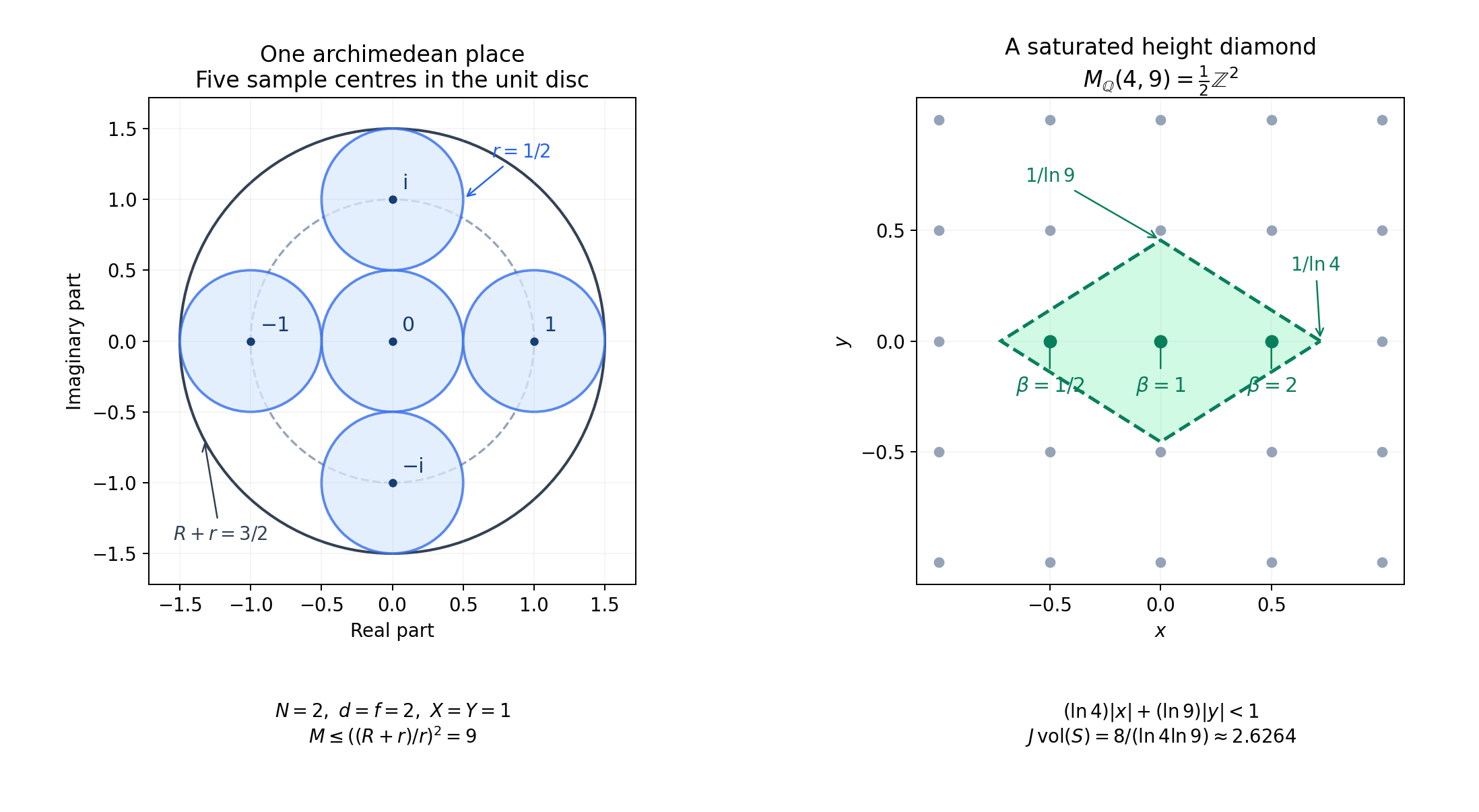
Figure 10.2. Left: the sample \(0,\pm1,\pm i\) in \(\mathbb Q(i)\) has multiplicative height one and lies in the unit disc. For \(N=2,d=f=2,X=Y=1\), Lemma 10.16 uses radius \(r=1/2\); the five small discs have disjoint interiors and lie in the disc of radius \(R+r=3/2\). The area bound is nine centres. Right: for the rational bases \(4,9\), the full lattice is \(\tfrac12\mathbb Z^2\). The open diamond \((\ln4)|x|+(\ln9)|y|<1\) has volume \(2/(\ln4\ln9)\); its coset average is \(8/(\ln4\ln9)\), between two and three. The zero coset contains the three displayed points, giving \(1/2,1,2\). Their two rational root-of-unity multiples are six distinct numbers of height below \(\mathrm e\). These are samples of the proved packing and averaging steps (10.50), (10.56), not numerical substitutes for the uniform bounds. Source mechanism: Loher and Masser, cited below. Reproducible source: height_counting_geometry.py.
10. One logarithm with its residue order
The one-dimensional case needs the order of the original residue class, rather than the size of a saturated residue group. Keeping that order and the local residue degree in the height inequality gives a sharper form of the one-logarithm bound.
Theorem 10.21 (the actual residue order). Let \(K\) have degree \(d\), and let \(\mathfrak p\) be a prime above \(p\), of ramification index \(e\) and residue degree \(f\). Normalize \(v_p(p)=1\) and \(\operatorname{ord}_{\mathfrak p}=e v_p\). Suppose \(\alpha\in K^*\) is a unit at \(\mathfrak p\), and let \(g=|\langle\bar\alpha\rangle|\) be the order of its nonzero residue class. If \(b\in\mathbb Z\setminus\{0\}\) and \(\alpha^b\ne1\), then
\[ \operatorname{ord}_{\mathfrak p}(\alpha^b-1) \le e v_p(b)+\frac d{f\ln p} \left(\frac{gep}{p-1}h(\alpha)+\ln2\right). \tag{10.59} \]Consequently,
\[ \operatorname{ord}_{\mathfrak p}(\alpha^b-1) \le\frac d{f\ln p} \left(\ln(2|b|)+g\left(1+\frac1{p-1}\right)e h(\alpha)\right). \tag{10.60} \]Both bounds include roots of unity, subject to the nonvanishing condition.
Proof. Replacing \(b\) by \(|b|\) does not change the valuation: for a unit \(x\), \(x^{-1}-1=-x^{-1}(x-1)\). Hence take \(b>0\). The order \(g\) divides \(p^f-1\), so it is prime to \(p\). If \(g\nmid b\), reduction makes the left side zero.
For every nonzero \(\eta\in K\), the normalized height formula gives
\[ \operatorname{ord}_{\mathfrak p}(\eta)\ln p \le\frac d f h(\eta). \]Indeed, when the valuation is positive, the contribution of \(\mathfrak p\) to \(d h(\eta^{-1})\) is \(f\operatorname{ord}_{\mathfrak p}(\eta)\ln p\), and all other contributions are nonnegative. Use \(h(\eta^{-1})=h(\eta)\). When it is nonpositive, the inequality is immediate. These are the height and local-degree identities proved in Heights of algebraic numbers and Places of number fields in extensions and the product formula.
First suppose \(\alpha\) is not a root of unity and \(g\mid b\). Put \(\beta=\alpha^g\). Its positive finite valuation \(v_p(\beta-1)\) is at least \(1/e\). Let \(t\) be the least nonnegative integer with \(p^t>e/(p-1)\). The proved entrance-time and power-step statements in p-adic logarithms: power series, heights and the one-logarithm bound give
\[ c_t=v_p(\alpha^{gp^t}-1)>\frac1{p-1}, \qquad p^t\le\frac{ep}{p-1}. \]The second inequality follows from minimality when \(t>0\). When \(t=0\), its right side is greater than one since \(e\ge1\).
Write \(b=g p^a m\), with \(p\nmid m\). Then \(a=v_p(b)\). Prime-to-\(p\) powers preserve positive valuation. After step \(t\), each \(p\)-power adds one. Earlier positive valuations increase strictly at each step, including a step on the boundary. Thus, whether \(a\ge t\) or \(a<t\),
\[ v_p(\alpha^b-1)\le a+c_t. \]Apply the local height inequality to \(\eta=\alpha^{gp^t}-1\ne0\). The proved height power and sum inequalities give \(h(\eta)\le gp^t h(\alpha)+\ln2\). Multiplying the preceding valuation bound by \(e\) therefore yields
\[ \operatorname{ord}_{\mathfrak p}(\alpha^b-1) \le e a+\frac d{f\ln p} \left(gp^t h(\alpha)+\ln2\right). \]Use \(p^t\le ep/(p-1)\) to obtain (10.59).
Now suppose \(\alpha\) is a root of unity. Its height is zero by the height power identity. If the left side is positive, the nontrivial root \(\alpha^b\) has \(p\)-power order: write its order as \(p^u s\), \(p\nmid s\), and use the prime-to-\(p\) power step to show that a root of order dividing \(s\) congruent to one must be one. The completely proved cyclotomic distance formula in the same lesson, Section 5 gives
\[ \operatorname{ord}_{\mathfrak p}(\alpha^b-1) \le\frac e{p-1}\le\frac{d\ln2}{f\ln p}. \]For the second inequality use \(ef\le d\) and \(\ln p\le(p-1)\ln2\), which follows by induction from \(p\le2^{p-1}\) for integers \(p\ge2\). This proves (10.59) for torsion as well.
Finally \(v_p(b)\ln p\le\ln|b|\) and \(ef\le d\), so \(e v_p(b)\le d\ln|b|/(f\ln p)\). Substitute in (10.59) and use \(p/(p-1)=1+1/(p-1)\) to obtain (10.60). \(\square\)
For example, take \(K=\mathbb Q\), \(\alpha=4\), \(p=5\). The original residue has order \(g=2\), while the saturated basis \(2\), together with \(-1\), generates all four nonzero residues. Thus (10.49) gives saturated index one, whereas the original one-dimensional residue index is two. The parameters serve different bounds.
The exact power laws give valuation zero for odd \(b\), and \(1+v_5(b)\) for even \(b\). For \(b=2\cdot5^k\), (10.60) reads
\[ 1+k\le k+\frac{7\ln4}{2\ln5}. \]At the torsion boundary, \(K=\mathbb Q\), \(p=2\), \(\alpha=-1\), \(b=1\), the height term vanishes and (10.60) is the equality \(1=\ln2/\ln2\).
Corollary 10.22 (a rational one-base reduction). Let \(\alpha_1,\ldots,\alpha_n\in K^*\) be units at \(\mathfrak p\), and let \(\zeta\in K\) be a root of unity of order \(w\). Let \(c_0,c_1,\ldots,c_n\) and \(b_1,\ldots,b_n\) be integers, with \(\boldsymbol b\ne0\), and suppose
\[ b_j=\frac uv c_j\quad(1\le j\le n), \qquad u\ne0,\quad v\ge1,\quad \gcd(u,v)=1. \]Put \(\gamma=\zeta^{c_0}\prod_j\alpha_j^{c_j}\), \(\Xi=\prod_j\alpha_j^{b_j}\), and \(B_*=\min_{b_j\ne0}|b_j|\). If \(\gamma\) is not a root of unity and \(\Xi\ne1\), then, with \(g_\gamma=|\langle\bar\gamma\rangle|\),
\[ \operatorname{ord}_{\mathfrak p}(\Xi-1) \le\frac d{f\ln p} \left(\ln(2wB_*)+ g_\gamma\left(1+\frac1{p-1}\right)e h(\gamma)\right). \tag{10.61} \]Proof. The coefficient identities give \(\Xi^v=\zeta^{-uc_0}\gamma^u\), and hence \(\Xi^{vw}=\gamma^{uw}\ne1\). All these numbers are local units. Factoring \(X^{vw}-1\) by \(X-1\) and evaluating at \(\Xi\) shows that \(\operatorname{ord}_{\mathfrak p}(\Xi-1)\le \operatorname{ord}_{\mathfrak p}(\gamma^{uw}-1)\): the remaining finite sum consists of integral units and is therefore integral. Apply (10.60) to \(\gamma\) and exponent \(uw\). Since \(v b_j=u c_j\) and \(u,v\) are coprime, \(u\) divides every \(b_j\). Thus \(|u|\le B_*\), proving (10.61). \(\square\)
This reduces a form whose coefficient vector is rationally proportional to one integral vector to a single unit, with an exact exponent budget. Applying it to a many-logarithm estimate also requires a proved bound for \(h(\gamma)\) in terms of the original heights; the saturation bounds of Section 9 supply one of the ingredients for that step.
11. Integral derivative bases and a multiplicity reduction
The many-logarithm argument changes the torus coordinates and then differentiates in a rational hyperplane. Two facts matter: the change of derivative basis must preserve p-adic integrality, and the zero estimate must allow different allocations of points at its different dimension steps. We establish both, keeping the coordinate degrees separate.
A minor of minimum valuation
Lemma 10.23 (integral derivative coordinates). Let \(2\le r\le n\). Suppose \(L_0=z_0,L_1,\ldots,L_r\) are independent integral linear forms, with \(L_i=a_{i0}z_0+\sum_{j=1}^n a_{ij}z_j\), and \(\sum_j b_jz_j=B_0L_0+\sum_{i=1}^rB_iL_i\), where \(b_j\in\mathbb Z\), \(B_i\in\mathbb Q\), \(b_n\ne0\), and \(B_r\ne0\). Set
\[ C_{ij}=b_n a_{ij}-b_j a_{in}\quad(1\le i\le r,\ 1\le j<n), \qquad E_i=Y_i\frac{\partial}{\partial Y_i}. \tag{10.62} \]The derivations
\[ \delta_j=\sum_{i=1}^rC_{ij}E_i =\frac1{B_r}\sum_{i<r}C_{ij}(B_rE_i-B_iE_r) \quad(1\le j<n) \tag{10.63} \]span the torus hyperplane \(\sum_iB_i x_i=0\), of dimension \(r-1\). Let \(C'\) be the first \(r-1\) rows of \(C\). Choose \(r-1\) columns \(J\) whose nonzero determinant has minimum \(v_p\) among all such minors. Then the corresponding \(\delta_j\), \(j\in J\), are independent, and every \(\delta_j\) has an expression
\[ \delta_j=\sum_{k\in J}\lambda_{kj}\delta_k, \qquad \lambda_{kj}\in\mathbb Q\cap\mathbb Z_p. \tag{10.64} \]Vanishing of all jets of total order at most \(T\) for these selected derivations and \(\partial_{Y_0}\) is therefore equivalent to vanishing for all the displayed derivations and \(\partial_{Y_0}\). The changes of jets have p-adically integral coefficients.
Proof. Comparing the coefficients of \(z_j\), \(j\ge1\), gives \(b_j=\sum_iB_i a_{ij}\). Hence \(\sum_iB_i C_{ij}=0\), proving the equality in (10.63).
The \(r\) row vectors \(a_i=(a_{i1},\ldots,a_{in})\) are independent. Otherwise a nonzero combination of the \(L_i\) would be a multiple of \(L_0\), contrary to the assumed independence. Suppose a combination \(a=\sum_{i<r}q_i a_i\) annihilates the vectors \(b_ne_j-b_je_n\), \(j<n\). Then \(b_n a_j-b_j a_n=0\) for every \(j<n\), so \(a=(a_n/b_n)b\). Since \(b=\sum_iB_i a_i\) and \(B_r\ne0\), row independence first forces \(a_n/b_n=0\), then all \(q_i=0\). Thus \(C'\) has rank \(r-1\). Its column images in the full matrix are determined by their first \(r-1\) coordinates through \(\sum_iB_i C_{ij}=0\). They span exactly the stated hyperplane.
Solve \(C'_j=C'_J\lambda_j\) by Cramer's rule. Each numerator is zero or, up to sign, another \((r-1)\)-column minor. Minimality of the chosen denominator's valuation therefore gives \(v_p(\lambda_{kj})\ge0\). This proves (10.64).
The Euler derivations commute with one another and with \(\partial_{Y_0}\). Expanding a product of the linear combinations (10.64) expresses every jet of order at most \(T\) as a combination of selected jets of that order. The coefficients are products and sums of the \(\lambda_{kj}\), multiplied by integer multinomial coefficients, so they are in \(\mathbb Z_p\). Conversely the selected derivations are among the original ones. This proves both directions of the vanishing assertion. \(\square\)
These operators also preserve the coordinate degree bounds and local integral coefficients. In fact, \(\delta_j(Y^{\boldsymbol m})=(\sum_iC_{ij}m_i)Y^{\boldsymbol m}\). For a polynomial of degrees at most \(D_i\ge1\), put \(M_j=\max\{1,\sum_i|C_{ij}|D_i\}\). On a monomial, the multiplier of \(\partial_{Y_0}^{t_0}\prod_j\delta_j^{t_j}\) is an integer, and its ordinary absolute value is at most
\[ D_0^{t_0}\prod_jM_j^{t_j}. \tag{10.65} \]Indeed the additive factor is the falling factorial of its exponent, bounded by \(D_0^{t_0}\), and each Euler factor has the displayed bound. Nonzero terms retain their torus exponents and lose exactly \(t_0\) in the additive exponent, so distinct input monomials do not merge. At finite places the integral multipliers introduce no new denominators.
Weighted relations with a sharp degree constant
We shall use the complete upper successive-minima inequality and subgroup-minor calculation in Modern estimates: Matveev and Waldschmidt. The following deduction uses the Euclidean radius \(1/\sqrt r\) in the weighted estimate.
Lemma 10.24 (weighted independent relations). Let \(\mathcal M\subseteq\mathbb Z^r\) have rank \(1\le\nu\le r\), with basis matrix \(U\) of size \(r\) by \(\nu\). Let \(A_j>0\). If \(|\det U_J|\prod_{j\in J}A_j\le B\) for every \(\nu\)-row set \(J\), there are independent \(u_1,\ldots,u_\nu\in\mathcal M\) with
\[ \prod_{i=1}^{\nu}\sum_jA_j|u_{ij}| \le K_{r,\nu}B,\qquad K_{r,\nu}=2^\nu(r/\pi)^{\nu/2} \Gamma(1+\nu/2)\binom r\nu^{1/2}\le r^\nu. \tag{10.66} \]They span \(\mathcal M_{\mathbb Q}\); an integral basis is not asserted.
Proof. Give its real span the weighted Euclidean metric \(\sum_jA_j^2x_j^2\). The Gram determinant identity gives covolume \((\sum_{|J|=\nu}\det(U_J)^2\prod_{j\in J}A_j^2)^{1/2}\le\binom r\nu^{1/2}B\). The unit ball of \(\sum_jA_j|x_j|\) contains the weighted Euclidean ball of radius \(1/\sqrt r\), by Cauchy–Schwarz. Its \(\nu\)-volume is therefore at least \((\pi/r)^{\nu/2}/\Gamma(1+\nu/2)\). The complete volume and upper successive-minima arguments in the earlier lesson give independent lattice vectors with product of these norms at most \(2^\nu\) times the covolume divided by that volume. This proves the first inequality.
For the second use \(\binom r\nu\le r^\nu/\nu!\). It suffices to show \(a_\nu=2^\nu\Gamma(1+\nu/2)/(\pi^{\nu/2}\sqrt{\nu!})\le1\). The Gaussian integral gives \(a_0=a_1=1\), and integration by parts in the defining gamma integral gives \[ \frac{a_{\nu+2}}{a_\nu}=\frac2\pi \sqrt{\frac{\nu+2}{\nu+1}}<1\quad(\nu\ge0), \] since \(\pi>3>2\sqrt2\). For completeness, \(\pi>3\) follows from \(\pi/4=\int_0^1(1+x^2)^{-1}\,dx\): the first eight terms of the integrated geometric series give the strict lower bound \(\sum_{j=0}^7(-1)^j/(2j+1)>3/4\). Its omitted remainder is the integral of \(x^{16}/(1+x^2)>0\). Thus both parity sequences decrease from one. This proves \(K_{r,\nu}\le r^\nu\). \(\square\)
Unequal allocations in the zero estimate
Let \(k\) be algebraically closed of characteristic zero, and put \(G=\mathbb G_a\times\mathbb G_m^r\). Write \(g^s=(s,\vartheta_1^s,\ldots,\vartheta_r^s)\), where the \(\vartheta_i\in k^*\) are multiplicatively independent. For nonzero \(\boldsymbol B\in\mathbb Q^r\), let \(W\) be the span of \(\partial_{Y_0}\) and the Euler directions in the hyperplane \(\boldsymbol B\cdot\boldsymbol x=0\). Its dimension is \(r\).
Theorem 10.25 (multiplicity and dimension reduction). Suppose \(r\ge2\), and let \(S,T\) be nonnegative integers. Choose nonincreasing nonnegative integer allocations
\[ S_0\ge\cdots\ge S_r,\quad T_0\ge\cdots\ge T_r,\qquad \sum_{m=0}^rS_m\le S,\quad\sum_{m=0}^rT_m\le T. \tag{10.67} \]Let the positive coordinate bounds \(D_0,\ldots,D_r\) satisfy \(D_0\ge\max\{D_1,\ldots,D_r,T_r+r\}\), and assume
\[ \begin{aligned} (S_m+1)\binom{T_m+m+1}{m+1} &>(m+1)!D_0 \max_{\substack{J\subseteq\{1,\ldots,r\}\\|J|=m}} \prod_{j\in J}D_j &&(0\le m<r),\\ (S_r+1)\binom{T_r+r}{r} &>(r+1)!D_0\prod_{j=1}^rD_j. \end{aligned} \tag{10.68} \]If a nonzero polynomial of these coordinate bounds vanishes at \(g^s\), \(0\le s\le S\), with all \(W\)-jets of total order at most \(T\), then there are \(1\le\nu<r\) and independent integral vectors \(u_1,\ldots,u_\nu\), whose rational span contains \(\boldsymbol B\). For any \(A_j>0\), put \(R_i=\sum_jA_j|u_{ij}|\) and \(C_{r,\nu}=\nu!K_{r,\nu}\le\nu!r^\nu\). At least one of
\[ (S_\nu+1)\binom{T_\nu+\nu-1}{\nu-1}\prod_iR_i \le C_{r,\nu}\max_{|J|=\nu}\prod_{j\in J}A_jD_j, \tag{10.69} \] \[ (S_\nu+1)\binom{T_\nu+\nu}{\nu}\prod_iR_i \le(\nu+1)C_{r,\nu}D_0 \max_{|J|=\nu}\prod_{j\in J}A_jD_j \tag{10.70} \]holds.
Proof. We use the fully proved stabilizer, jet and coordinate-degree arguments of the multiplicity subsection of the earlier lesson, explaining the allocation step explicitly. Let \(N=r+1\). For \(1\le j\le N+1\), let \(I_j\) be generated by the translates of all \(W\)-derivatives of \(P\) of order at most \(\sum_{m=0}^{j-2}T_m\), at translating points \(g^s\) with \(0\le s\le\sum_{m=0}^{j-2}S_m\); empty sums are zero. Write \(X_j=Z(I_j)\). Translations and invariant derivatives preserve the coordinate bounds. Hence \(G\supsetneq X_1\supseteq\cdots\supseteq X_{N+1}\), and the last set contains the identity by (10.67). Every set is nonempty.
Choose the first \(j\) for which \(X_j,X_{j+1}\) have the same dimension, and a common component \(V\) of that dimension. Such a \(j\le N\) exists, since \(\dim X_1\le N-1\). Before it each dimension falls, so \(\dim V\le N-j\). As in the cited stabilizer proof, define \(E=\{x:x+V\subseteq X_j\}\) and \(H=\{x:x+V=V\}\). The set \(E\) is a finite union of \(H\)-cosets. Its defining ideal, obtained by translating the generators of \(I_j\) by \(V\), has dimension \(\dim H\) and the same coordinate degree bounds. That ideal vanishes through order \(T_{j-1}\) on \(\{g^s:0\le s\le S_{j-1}\}+H\), because the added derivatives and translates are among those defining \(X_{j+1}\).
Replace \(H\) by its identity component \(H_0\), and put \(c=N-\dim H_0\). Since \(\dim H_0\le\dim V\), we have \(c\ge j\). Monotonicity gives at least \(S_{c-1}+1\) point cosets and at least \(T_{c-1}\) jets on them. All these cosets are distinct. Indeed, if \(g^q\in H_0\) for \(q\ne0\), the nonzero additive coordinate forces the additive part of \(H_0\) to be \(\mathbb G_a\). Properness then supplies a nonzero torus character \(u\) with \(\boldsymbol\vartheta^{qu}=1\), contrary to multiplicative independence.
Put \(\sigma=\dim(W/(W\cap T(H_0)))\). The complete positive-filtration upper and lower estimates (8.72)–(8.76) give, for every codimension-\(c\) coordinate set \(J\),
\[ (S_{c-1}+1)\binom{T_{c-1}+\sigma}{\sigma}\delta(H_0;J) \le c!\prod_{j\in J}D_j. \tag{10.71} \]Here \(\delta(H_0;J)\) is the nonnegative integral coefficient of the complementary monomial in the subgroup Hilbert polynomial. To extract a coefficient from the lower polynomial inequality, send exactly the coordinates in that complementary monomial to a common infinity, keeping the others one. The polynomials are squarefree of the same degree, so division by that power leaves exactly the desired coefficient. This is the coefficient argument already proved in the earlier lesson.
Since \(W\) is a hyperplane, \(\sigma=c-1\) when \(T(H_0)\subseteq W\), and \(\sigma=c\) otherwise. In the second case \(c\le r\), and some \(\delta\) is at least one. The maximum product of \(c\) coordinate bounds is \(D_0\max_{|J|=c-1}\prod_{j\in J}D_j\), because \(D_0\) is largest. Inequality (10.71) contradicts (10.68) with \(m=c-1\). Hence \(T(H_0)\subseteq W\).
Write \(H_0=H_a\times H_m\), and let \(\mathcal M\) be the primitive character lattice of \(H_m\), of rank \(\nu\). The subgroup and tangent classification in the earlier lesson shows that \(\boldsymbol B\in\mathcal M_{\mathbb Q}\). Thus \(\nu\ge1\). If \(\nu=r\) and \(H_a=\{0\}\), then \(c=r+1,\sigma=r\), and (10.71) contradicts the last line of (10.68). If \(\nu=r\) and \(H_a=\mathbb G_a\), then \(c=r,\sigma=r-1\). We may decrease the available budgets to \(S_r,T_r\); its unique torus coefficient is one. Thus \((S_r+1)\binom{T_r+r-1}{r-1}\le r!\prod_{j=1}^rD_j\). The last line of (10.68), and \(\binom{T_r+r}{r}/\binom{T_r+r-1}{r-1}=(T_r+r)/r\), contradict this since \(D_0\ge T_r+r\). Therefore \(1\le\nu<r\).
Let \(U\) be a basis matrix of \(\mathcal M\). If \(H_a=\mathbb G_a\), the subgroup coefficients are \(|\det U_J|\), \(c=\nu,\sigma=\nu-1\). Decrease its budgets to \(S_\nu,T_\nu\). Multiply (10.71) by \(\prod_{j\in J}A_j\), and apply Lemma 10.24 to the resulting bounds on every weighted minor. The independent vectors supplied by that lemma span \(\mathcal M_{\mathbb Q}\), so their span contains \(\boldsymbol B\). Its factor \(K_{r,\nu}\) times \(\nu!\) gives (10.69). If \(H_a=\{0\}\), then \(c=\nu+1,\sigma=\nu\); its coefficients on \(\{0\}\cup J\) are \(|\det U_J|\). The same argument uses \((\nu+1)!D_0\) in (10.71), proving (10.70). This accounts for both additive subgroups and completes the proof. \(\square\)
For the allocations \(S_0=\lfloor S/3\rfloor\), \(S_i=\lfloor2S/(3r)\rfloor\) for \(i\ge1\), and \(T_i=\lfloor T/(r+1)\rfloor\), (10.67) holds: \(r\ge2\) makes the point allocations nonincreasing, and their sums are at most \(S,T\). Since the \(T_i\) are equal and \(D_0\ge T_r+r\), (10.69) also implies (10.70). Multiply (10.69) by \((T_\nu+\nu)/\nu\le D_0\); its enlarged right side is at most the right side of (10.70). Thus the second bound alone suffices for this choice of allocations.
Corollary 10.26 (new algebraic bases). If the \(\vartheta_j\) are independent algebraic units in a number field and \(u_i\) are the vectors in Theorem 10.25, put \(\gamma_i=\prod_j\vartheta_j^{u_{ij}}\). They are independent units and
\[ h(\gamma_i)\le\sum_j|u_{ij}|h(\vartheta_j)\le R_i \quad\text{if }A_j\ge h(\vartheta_j). \tag{10.72} \]If \(\boldsymbol b\in\mathbb Z^r\) is in their rational span, there are integers \(m\ge1,c_i\) with \(m\boldsymbol b=\sum_i c_i u_i\), and \((\prod_j\vartheta_j^{b_j})^m=\prod_i\gamma_i^{c_i}\).
Proof. Integer products preserve local units, and the proved height power and product inequalities give (10.72). A multiplicative relation among the \(\gamma_i\) gives a zero integral combination of the \(u_i\), by independence of the \(\vartheta_j\); linear independence of the vectors makes every coefficient zero. Clearing the denominators of a rational span expression proves the last identity. \(\square\)
Example of a sharp weighted factor. For \(r=2,\nu=1\), take \(\mathcal M=\mathbb Z(3,-2)\), weights \(A_1=2,A_2=3\), and minor bound \(B=6\). Its primitive vector has weighted norm 12, exactly \(K_{2,1}B=2B\). In the torus put \(H_m=\{Y_1^3=Y_2^2\}\), \(H=\mathbb G_a\times H_m\), and \(g=(1,2,3)\). For \(s=0,1,2\), its three distinct \(H\)-cosets have characters \(Y_1^3/Y_2^2=(8/9)^s\). The polynomial \[ P(Y_1,Y_2)=\prod_{s=0}^2(9^sY_1^3-8^sY_2^2) \] vanishes on all three. The directions \(\partial_{Y_0}\) and \(2E_1+3E_2\) are tangent to these cosets, so every such derivative vanishes there. Its coordinate bounds are \(D_1=9,D_2=6\), and the corresponding weighted relation inequality is the equality \(3\cdot12=2\max(2\cdot9,3\cdot6)=36\). There is no transverse multiplicity factor in this case: \(\sigma=\nu-1=0\).
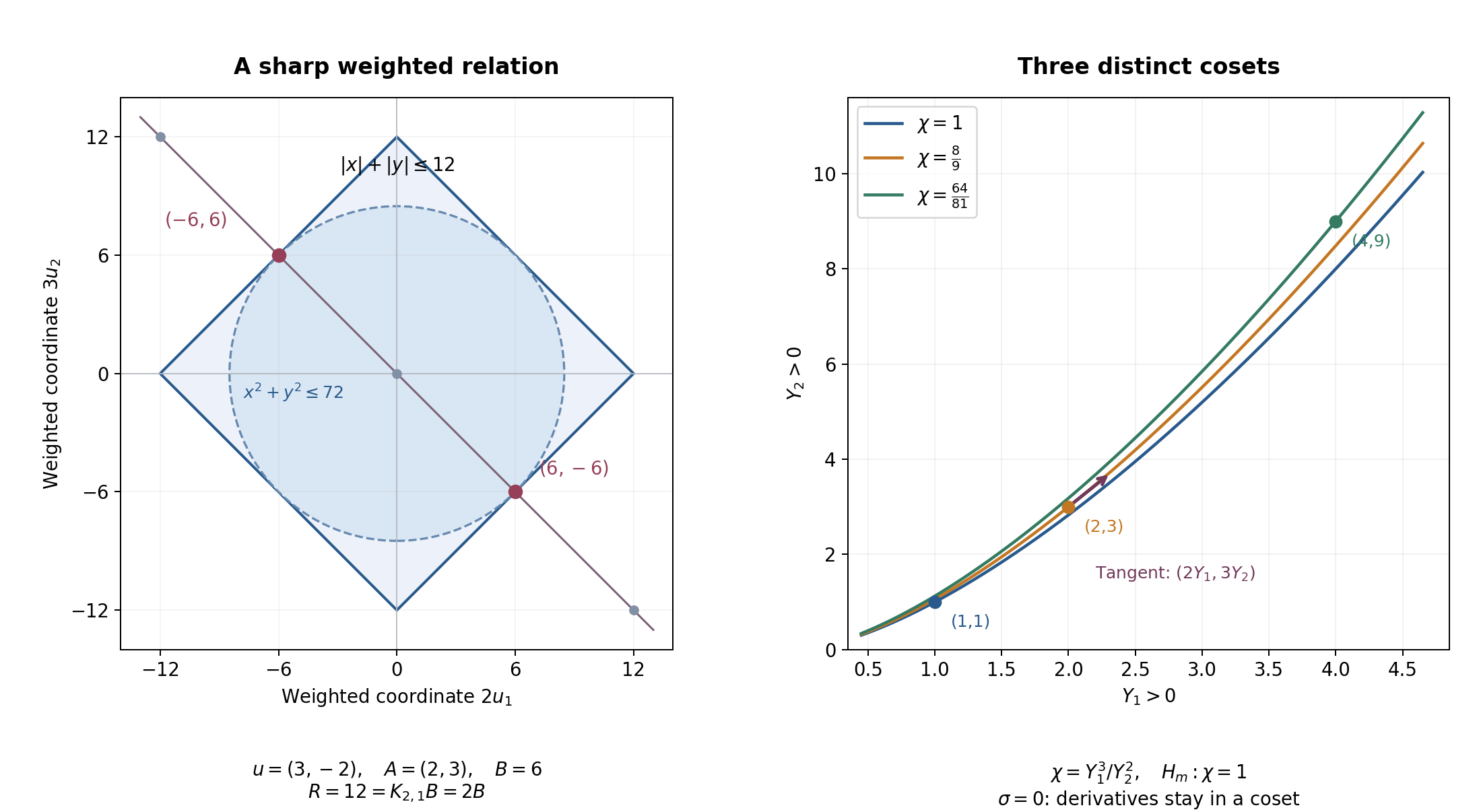
Figure 10.3. Left: in weighted coordinates \((2u_1,3u_2)\), the relation \((3,-2)\) becomes \((6,-6)\). Its diamond norm is 12; the Euclidean circle of radius \(12/\sqrt2\) lies in the diamond and meets that relation line at the two marked primitive vectors. This is the equality case of (10.66) for \(r=2,\nu=1\). Right: a positive real section of the torus projections of the three cosets above. Their quotient character values \(1,8/9,64/81\) are distinct, and the points \((1,1),(2,3),(4,9)\) lie on their respective curves. The additive coordinates \(0,1,2\) are omitted from this projection. The arrow is tangent to a coset, in the direction \(2E_1+3E_2\); it illustrates \(\sigma=0\), not a transverse derivative. The complete subgroup, degree and lattice arguments are (10.66), (10.69)–(10.71) and the example. Mathematical background: the earlier complete multiplicity lesson and Yu's free 2013 article, cited below. Figure program.
12. Closing the one-base branch
The many-logarithm construction may reduce to one new base before the auxiliary polynomial is needed. A one-logarithm inequality alone does not finish that step: its constant term must also be compared with the product of the original heights. We give that comparison with the full residue-order and root-of-unity factors.
Let \(n\ge2\), let \(K\) have degree \(d\), and let \(\mathfrak p\) lie above \(p\), with ramification index \(e_{\mathfrak p}\) and residue degree \(f\). Put \(t=f\ln p\) and \(\ln^*d=\max\{1,\ln d\}\). Take multiplicatively independent \(\mathfrak p\)-adic units \(\alpha_1,\ldots,\alpha_n\), integers \(b_j\) not all zero, and write
\[ \Xi=\prod_j\alpha_j^{b_j},\qquad P_h=\prod_jh(\alpha_j),\qquad B_* =\min_{b_j\ne0}|b_j|. \tag{10.73} \]Take \(q=2\) for \(p>2\), and \(q=3\) for \(p=2\). In the second case assume \(\zeta_3\in K\). Let \(w_q=q^u\) be the order of the q-primary roots of unity in \(K\), and choose their generator \(\alpha_0\). Use the intrinsic saturated residue index \(\delta(\boldsymbol\alpha)\) from Lemma 10.15, and define
\[ \begin{aligned} Q_n&=p^f/\delta(\boldsymbol\alpha),& M_n&=\max\{Q_n/t^{n+1},\mathrm e^n/n^n\},\\ L&=\max\{\ln(\mathrm e^4(n+1)d),e_{\mathfrak p},t\},& \varepsilon_n&=10^{-26}/(2n),\\ a&=\begin{cases} 7(p-1)/(p-2),&p\ge5,\ e_{\mathfrak p}=1,\\ 14,&p>2\text{ in the other cases},\\ 26,&p=2, \end{cases}& R_n&=\frac{\mathrm e a}{q}(1+\varepsilon_n)(n+1)d. \end{aligned} \tag{10.74} \]Here \(\mathrm e=\exp(1)\) is distinct from the ramification index. For any \(c\ge206\), put
\[ \mathcal C_n= c a^n\frac{n^n(n+1)^{n+1}d^{n+2}\ln^*d} {n!w_qt}\,M_nL. \tag{10.75} \]Theorem 10.27 (the one-base numerical closure). Suppose there are independent integral forms \(L_0=z_0,L_1=a_0z_0+\sum_ja_jz_j\), and rationals \(B_0,B_1\), with \(B_1\ne0\), such that \(\sum_jb_jz_j=B_0L_0+B_1L_1\). Set \(\gamma=\alpha_0^{a_0}\prod_j\alpha_j^{a_j}\), and let \(g_\gamma\) be its actual residue order at \(\mathfrak p\). Define
\[ \delta_\gamma=\frac{p^f-1}{g_\gamma},\qquad M_\gamma=\max\{p^f/(\delta_\gamma t^2),\mathrm e\}. \tag{10.76} \]Suppose a positive \(\sigma\) satisfies
\[ h(\gamma)\le\sigma\le R_n^{n-1}\frac{M_n}{M_\gamma}P_h. \tag{10.77} \]If \(H\ge\max\{\ln B_*,(n+1)t,\ln(4d)\}\), then
\[ \operatorname{ord}_{\mathfrak p}(\Xi-1) \le\frac1{500}\mathcal C_nP_hH <\mathcal C_nP_hH. \tag{10.78} \]Proof. Write \(B_1=v_1/v_2\) in lowest terms, with \(v_2>0\). Coefficient comparison gives \(v_2b_j=v_1a_j\); hence \(v_1\mid b_j\) and \(|v_1|\le B_*\). Also \(v_2B_0=-v_1a_0\) is integral. Raising the resulting multiplicative identity to \(w_q\) removes \(\alpha_0\): \(\Xi^{v_2w_q}=\gamma^{v_1w_q}\).
The vector \((a_1,\ldots,a_n)\) is nonzero, by independence of the two forms. Thus \(\gamma\) is not a root of unity: a torsion relation would, after a further power killing \(\alpha_0\), contradict independence of the \(\alpha_j\). The same argument proves that \(\Xi\) is not torsion. All powers just used are therefore different from one. The finite geometric sum and Theorem 10.21 give
\[ \operatorname{ord}_{\mathfrak p}(\Xi-1) \le\frac d t\left( \ln(2w_q B_*)+ g_\gamma\frac p{p-1}e_{\mathfrak p}h(\gamma)\right). \tag{10.79} \]Negative \(v_1\) is covered by that theorem. The geometric sum has integral local-unit terms, so its valuation is nonnegative.
We need two elementary estimates. First,
\[ w_q\le\frac q{q-1}d\le2d. \tag{10.80} \]Indeed Proposition 9.7, applied at the prime \(q\), proves that \(\Phi_{q^u}\) is irreducible over \(\mathbb Q_q\), of degree \(q^{u-1}(q-1)\). It is consequently irreducible over \(\mathbb Q\) as well. Since its root \(\alpha_0\) belongs to \(K\), that degree is at most \(d\), proving (10.80). Thus \(\ln(2w_qB_*)\le2H\).
Second, if \(w_K\) is the total number of roots of unity in \(K\), Theorem 10.18 and the index lower bound one give the uniform weakened form
\[ P_h\ge \frac{w_K n^n} {58 n!\mathrm e^n d^{n+1}\ln^*d} \ge\frac{w_q n^n} {58 n!\mathrm e^n d^{n+1}\ln^*d}. \tag{10.81} \]For \(d=1\), the proved constant 17 is smaller than 58, so the same form holds. There is no lower bound for a single new height hidden in this step.
Combining (10.75), (10.81) and \(M_n\ge\mathrm e^n/n^n\) gives
\[ \mathcal C_nP_h\ge \frac c{58}a^n \frac{n^n(n+1)^{n+1}}{(n!)^2}\frac d tL \ge\frac c{58}a^n(n+1)\frac d tL >2000\frac d t. \tag{10.82} \]Here \(n!\le n^n\), \((n+1)^{n+1}/n^n\ge n+1\), \(a\ge7\), and \(L\ge4+\ln3>5\). The last numerical comparison is \(206\cdot49\cdot3\cdot5>2000\cdot58\). The logarithmic term in (10.79) is therefore at most \(\mathcal C_nP_hH/1000\).
For the height term use \(g_\gamma/M_\gamma<t^2\), directly from (10.76), and (10.77). Its ratio to \(\mathcal C_nP_hH\) is at most
\[ \frac{n!}{n^n}\left(\frac{\mathrm e}{q}\right)^{n-1} (1+\varepsilon_n)^{n-1} \frac{w_q e_{\mathfrak p}t^2} {c a(n+1)^2d^2\ln^*d\,LH}\frac p{p-1}. \tag{10.83} \]This is an exact cancellation of the \(M_n\), degree and exponential factors. The local degree inequality gives \(e_{\mathfrak p}\le d\); also \(L\ge t\), \(H\ge(n+1)t\), \(p/(p-1)\le2\), and (10.80) gives \(w_q/d\le2\).
For completeness, monotonicity of \(\ln x\) gives \(\ln(n!)\le\int_1^n\ln x\,dx+\ln n =n\ln n-n+1+\ln n\). Consequently \(n!\mathrm e^{n-1}/n^n\le n\). Furthermore \((1+\varepsilon_n)^{n-1}<2\): use \(\ln(1+x)\le x\), which follows by integrating \((1+x)^{-1}\le1\), and \(\varepsilon_n(n-1)<1/2\). The exponential series gives \(\mathrm e<3\), since \(k!\ge2^{k-1}\) for \(k\ge2\), with strict inequality for \(k\ge3\); hence \(\exp(1/2)<2\). This also proves \(\ln3>1\) used above.
Thus (10.83) is at most \(8n/(q^{n-1}c a(n+1)^3)\le4n/(c a(n+1)^3)\), because \(q\ge2,n\ge2\). Since \((n+1)^2\ge4n\) and \(n+1\ge3\), this is at most \(1/(3ca)\le1/(3\cdot206\cdot7)<1/1000\). The height term is also at most \(\mathcal C_nP_hH/1000\). Adding the two terms proves (10.78). \(\square\)
We check the correspondence with the free 2013 preparation. Let \(\kappa\) be the unique nonnegative integer with \(p^{\kappa-1}(p-1)\le2e_{\mathfrak p}<p^\kappa(p-1)\). Set \(c_2=7/4\) for \(p>2\), and \(c_2=13/9\) for \(p=2\). Put \(\vartheta=(p-2)/(p-1)\) when \(p\ge5,e_{\mathfrak p}=1\), and \(\vartheta=p^\kappa/(2e_{\mathfrak p})\) otherwise, and let \(\theta=\vartheta/(1+\varepsilon_n)\). Direct substitution gives
\[ \mathrm e c_2q\frac{p^\kappa}{e_{\mathfrak p}\theta}(n+1)d=R_n. \tag{10.84} \]In the first case \(\kappa=0\); in the other cases the factors are respectively \(7\) and \(26/3\) before multiplication by \(\mathrm e(1+\varepsilon_n)(n+1)d\). Thus (10.77) is precisely the one-base height-product hypothesis of that preparation. Formula (10.75) is its first numerical coefficient, with any of its listed choices of \(c\), all at least 206. Its parameter \(h^{(1)}\) is at least \(\ln B_*\) and \((n+1)t\); its term \((n+1)(a_0^{(1)}n+a_1^{(1)}+\ln(a_0^{(1)}n+a_2^{(1)})+\ln d)\) is larger than \(\ln(4d)\), since the listed constants satisfy \(a_0^{(1)}>3,a_1^{(1)}>2,a_2^{(1)}>2\). Theorem 10.27 therefore proves the full numerical conclusion in this branch. The proof retains the original saturated index for the \(n\) bases, and the actual unsaturated residue order for the one new base.
13. Binomial preparation of the auxiliary polynomial
The auxiliary polynomial uses shifted powers of binomial polynomials and binomial polynomials in the Euler eigenvalues. We prove their independence, their exact denominator control and their equivalence to ordinary jets. These are algebraic statements; no logarithm estimate is assumed in their proofs.
Taylor coefficients at integral and fractional nodes
For integers \(k\ge1,\ell\ge1,m\ge0\), define
\[ \begin{aligned} \Delta(z;k)&=\frac{(z+1)\cdots(z+k)}{k!},\quad \Delta(z;0)=1,\\ v(k)&=\operatorname{lcm}(1,\ldots,k),\\ \Theta(z;k,\ell,m)&=\frac1{m!}\frac{d^m}{dz^m}\Delta(z;k)^\ell. \end{aligned} \tag{10.85} \]Lemma 10.28 (prepared Taylor integrality). For every integer \(s\),
\[ v(k)^m\Theta(s;k,\ell,m)\in\mathbb Z. \tag{10.86} \]If \(q\) is prime, \(I\in\mathbb Z_{\ge0}\), and \(A,s\in\mathbb Z\), then
\[ q^{\chi_I\ell(kI+v_q(k!))}v(k)^m \Theta(s/q^I+A;k,\ell,m)\in\mathbb Z, \qquad \chi_0=0,\quad\chi_I=1\ (I>0). \tag{10.87} \]In particular \(v(k)^m\Theta(s/q^I+A;k,\ell,m)\) belongs to \(\mathbb Z[1/q]\), before multiplication by the displayed q-power.
Proof. Generalized binomial coefficients \(\binom Nj\) are integral for every integer \(N\): for \(N<0\), their product formula is \((-1)^j\binom{-N+j-1}j\). Vandermonde's polynomial identity gives \(\Delta(s+Z;k)=\sum_{j=0}^k\binom{s+k}{k-j}\binom Zj\). One proof first counts subsets for nonnegative integer arguments and then uses polynomial equality to extend to all arguments. For \(j\ge1\), \[ \binom Zj=\frac{(-1)^{j-1}Z}{j} \prod_{a=1}^{j-1}(1-Z/a). \] Each coefficient of \(Z^m\) has denominators consisting of \(j\) and \(m-1\) numbers among \(1,\ldots,j-1\). Every factor divides \(v(k)\). Hence multiplication by \(v(k)^m\) makes that coefficient integral. The constant coefficient is integral too. In the \(\ell\)-th power, a coefficient of order \(m\) is a sum of products whose orders sum to \(m\); the same scaling therefore clears all of them. This proves (10.86), including vanishing coefficients beyond the degree.
Fix \(F(Z)=v(k)^m\Theta(Z;k,\ell,m)\). It is a rational polynomial, integral at every integer. At \(x=s/q^I+A\), it has no denominator at a prime \(r\ne q\). To see this without a limiting argument, choose \(B\) bounding the r-adic denominators of its finitely many coefficients, and an integer \(N\equiv x\pmod{r^{B+1}}\); the inverse of \(q^I\) modulo that power supplies \(N\). Both \(x,N\) are r-integral. Factoring \(x^j-N^j\) shows that \(F(x)-F(N)\) is r-integral, so \(F(x)\) is r-integral.
The coefficients of \(\Delta(Z;k)^\ell\) have denominator dividing \((k!)^\ell\). Dividing an ordinary derivative of order \(m\) by \(m!\) multiplies each monomial coefficient by an integer binomial coefficient and decreases its degree by \(m\). Thus its value at \(x\) has q-adic denominator at most \(q^{\ell v_q(k!)+Ik\ell}\); the integer factor \(v(k)^m\) cannot worsen this bound. Together with the preceding assertion at every other prime this proves (10.87) for \(I>0\). For \(I=0\), (10.86) already gives an integer and no q-factor is needed. \(\square\)
Independence of the shifted powers
Lemma 10.29 (a binomial polynomial basis). For \(k,L\ge1\), the \(kL\) polynomials
\[ F_{a,\ell}(X)=\Delta(X+a;k)^\ell, \qquad 0\le a<k,\quad1\le\ell\le L, \tag{10.88} \]are a basis of the polynomials of degree at most \(kL\) vanishing at \(X=-k\). For fixed \(\ell\), their top \(k\) coefficient matrix satisfies
\[ \det\left([X^{k\ell-j}]F_{a,\ell}\right)_{0\le j,a<k} =\frac{\prod_{j=0}^{k-1}\binom{k\ell}{j}} {(k!)^{k\ell}}\prod_{0\le a<b<k}(b-a)\ne0. \tag{10.89} \]Proof. The coefficient in row \(j\), regarded as a polynomial in \(a\), has degree \(j\) and leading coefficient \(\binom{k\ell}j/(k!)^\ell\). Indeed expand the degree-\(k\ell\) polynomial \(\Delta(X;k)^\ell\) after substituting \(X+a\); its highest term gives that leading coefficient, and lower terms give smaller powers of \(a\). Changing these row polynomials to monomials is triangular. The monomial evaluation determinant at \(0,\ldots,k-1\) is the Vandermonde product in (10.89). It follows either by subtracting columns and induction, or by observing its zeros at equal columns and its leading coefficient one. This proves the formula.
In a proposed relation, take the largest \(\ell\) occurring. Lower levels have degree at most \(k(\ell-1)\). The top \(k\) coefficients and (10.89) force every coefficient at this largest level to vanish. Descending proves independence. Every polynomial in (10.88) vanishes at \(-k\), because the factor with index \(k-a\) is zero there. The space with this one vanishing condition has dimension \(kL\): evaluation at \(-k\) is a nonzero linear functional on the \(kL+1\)-dimensional polynomial space. Thus the independent family is a basis. An invertible affine substitution preserves its independence. \(\square\)
For \(k=L=2\), Figure 10.4 shows the four basis polynomials and their exact coefficient matrix. A shared root does not give a relation among the polynomials.
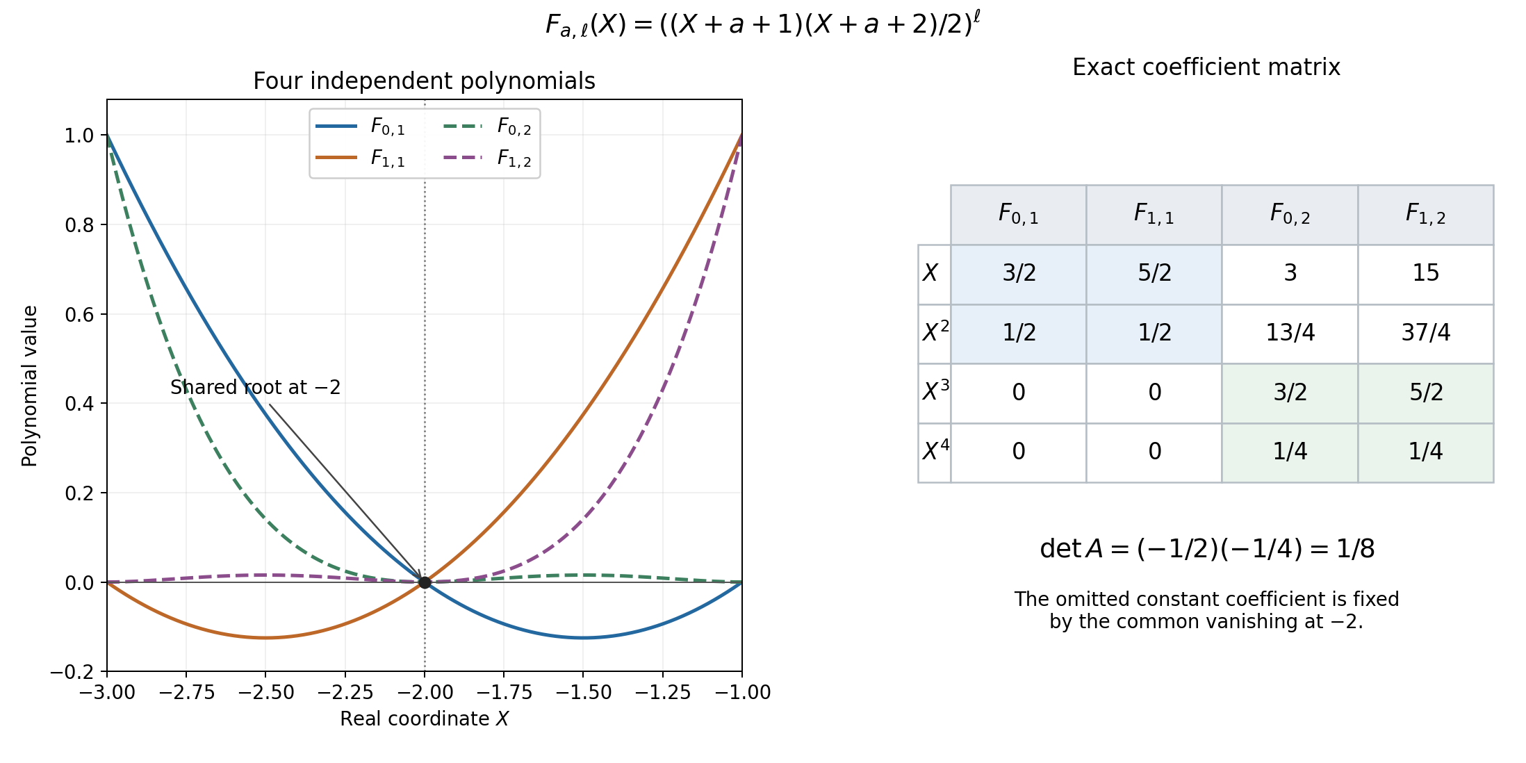
Figure 10.4. Left: the restrictions to the real interval \([-3,-1]\) of \(F_{0,1},F_{1,1},F_{0,2},F_{1,2}\) in (10.88) for \(k=2\). All vanish at \(-2\); the squared polynomials have a double zero there. Right: their coefficients of \(X,X^2,X^3,X^4\), in the same column order. The diagonal two-by-two block determinants are \(-1/2,-1/4\), so the full determinant is \(1/8\). Their constant coefficients are determined by their common vanishing at \(-2\). This is the exact independence mechanism in Lemma 10.29 and (10.89), applied to the auxiliary polynomial below. Human-source background: the binomial preparation in Yu's free 2013 article, cited below. Figure program.
Affine changes of binomial jets
Lemma 10.30 (Newton reparametrization). Over a characteristic-zero field, for \(h\ne0\) and \(c\),
\[ \Delta(hZ+c;t)=\sum_{j=0}^t d_j\Delta(Z;j),\qquad d_j=\sum_{i=0}^j(-1)^i\binom ji\Delta(c-h(i+1);t), \qquad d_t=h^t. \tag{10.90} \]If \(h,c\in\mathbb Z[1/q]\), then all \(d_j\) belong to that ring. If moreover \(h=q^b\), \(b\in\mathbb Z\), the triangular change and its inverse are p-adically integral for every \(p\ne q\). Products in several commuting variables preserve the total-order filtration.
Proof. The polynomials \(\Delta(Z;j)\), \(0\le j\le t\), have degrees \(j\) and nonzero leading coefficients, so form a basis. At \(Z=-i-1\), their values are \((-1)^j\binom ij\), zero when \(j>i\). Inverting this triangular evaluation matrix gives (10.90). Explicitly the inner binomial inversion sum is \(\binom ab\sum_{i=b}^a(-1)^{i-b}\binom{a-b}{i-b}\), which is zero for \(a>b\) and one for \(a=b\), by \((1-1)^{a-b}\). Comparing leading coefficients gives \(d_t=h^t\).
Lemma 10.28 with \(\ell=1,m=0\) makes each displayed value at a \(\mathbb Z[1/q]\) argument belong to that ring; the sum for \(d_j\) does too. When \(h=q^b\), the diagonal \(h^t\) is a unit in \(\mathbb Z[1/q]\). Successive substitution therefore also puts the inverse matrix in that ring, hence in \(\mathbb Z_p\) for \(p\ne q\). In products, every new index is coordinatewise at most the old one, so its total order cannot increase. \(\square\)
The integrality assertion here concerns changes between binomial families. Conversion between a binomial family and ordinary powers has leading coefficient \(1/t!\); we use that conversion only for algebraic equivalence of vanishing.
From prepared equations to the ordinary zero estimate
Proposition 10.31 (the auxiliary polynomial and its jets). Let \(\mathcal M\subset\mathbb Z^r\) be finite, with distinct exponent vectors \(\boldsymbol m\), and let \(A_i\ge0\) bound \(|m_i|\). Put \(d_i=\lfloor A_i\rfloor\). Fix \(q,I,k,L\) as above, and coefficients \(c_{\boldsymbol m,a,\ell}\) in a characteristic-zero field, not all zero. Form
\[ Q(X,Y)=\sum_{\boldsymbol m\in\mathcal M} \sum_{0\le a<k,\,1\le\ell\le L} c_{\boldsymbol m,a,\ell}\Delta(q^{-I}X+a;k)^\ell Y^{\boldsymbol m}, \qquad P=Y^{\boldsymbol d}Q. \tag{10.91} \]Then \(P\) is nonzero, is an ordinary polynomial, and has coordinate bounds \(kL,2A_1,\ldots,2A_r\).
Let \(D_j=\sum_i C_{ij}Y_i\partial_{Y_i}\) be commuting Euler derivations, and put \(\omega_j(\boldsymbol m)=\sum_iC_{ij}m_i\), \(1\le j\le r-1\). For a torus point \(\boldsymbol y\) define the prepared value
\[ \mathcal Q(s;\boldsymbol t)= \sum_{\boldsymbol m,a,\ell}c_{\boldsymbol m,a,\ell} v(k)^{t_0}\Theta(q^{-I}s+a;k,\ell,t_0) \prod_{j=1}^{r-1}\Delta(\omega_j(\boldsymbol m);t_j) \boldsymbol y^{\boldsymbol m}. \tag{10.92} \]For any \(T\), vanishing of all these values with \(|\boldsymbol t|\le T\) is equivalent to vanishing of all ordinary jets of \(Q\), and hence of \(P\), at \((s,\boldsymbol y)\) for \(\partial_X,D_1,\ldots,D_{r-1}\) through total order \(T\).
Proof. Distinct Laurent monomials are linearly independent. For each fixed \(\boldsymbol m\), Lemma 10.29, with the invertible substitution \(X\mapsto q^{-I}X\), proves independence of its coefficient polynomials. Thus not all coefficients can cancel, and \(Q\ne0\). Since \(m_i\) is integral and \(m_i\ge-A_i\), it satisfies \(m_i\ge-\lfloor A_i\rfloor\). Hence \(0\le m_i+d_i\le2A_i\). This proves the degree and nonvanishing assertions for \(P\).
On its monomial terms, (10.92) is exactly the value of the commuting operator \((q^Iv(k))^{t_0}\partial_X^{t_0}/t_0!\) times \(\prod_j\Delta(D_j;t_j)\), applied to \(Q\). The chain rule supplies \(q^{-It_0}\), canceled by \(q^{It_0}\). Each \(\Delta(D_j;t_j)\) has leading term \(D_j^{t_j}/t_j!\) and only lower powers. All diagonal scalars are nonzero. Induction on the torus part of the total order therefore makes these operators and the ordinary jet operators span exactly the same filtered space. This proves the first equivalence, in both directions.
Put \(c_j=\sum_iC_{ij}d_i\). The product rule gives
\[ \partial_X^{t_0}\prod_jD_j^{t_j}P =Y^{\boldsymbol d}\partial_X^{t_0} \prod_j(D_j+c_j)^{t_j}Q. \tag{10.93} \]Expanding is triangular with diagonal one and preserves total order. The inverse uses \(-c_j\) and \(Y^{-\boldsymbol d}\). Since every torus coordinate is nonzero, evaluation proves the second equivalence. \(\square\)
When the \(C_{ij}\) are integers, \(s\) is integral and \(q\ne p\), Lemma 10.28 and integer-valued \(\Delta\) give \[ v(k)^{t_0}\Theta(q^{-I}s+a;k,\ell,t_0) \prod_j\Delta(\omega_j(\boldsymbol m);t_j) \in\mathbb Z[1/q]\subseteq\mathbb Z_p. \] The prepared product \(v(k)^{t_0}\Theta\), rather than \(\Theta\) alone, needs at most the q-denominator in (10.87). Integrality of the whole value additionally requires locally integral \(c_{\boldsymbol m,a,\ell}\) and local-unit torus coordinates.
For the application to Theorem 10.25, take \(D_1,\ldots,D_{r-1}\) to be the selected integral Euler directions in Lemma 10.23, renumbered. They span the Euler hyperplane in that theorem's space \(W\). Apply the proposition at \((s,\vartheta_1^s,\ldots,\vartheta_r^s)\). All prepared equations then give precisely the ordinary \(W\)-jets required there, with
\[ D_0=kL,\qquad D_i=2A_i, \qquad A_i=q^{\nu-I}D_i^{\mathrm{old}},\quad k=D_{-1}^{\mathrm{old}}+1,\quad L=D_0^{\mathrm{old}}+1. \tag{10.94} \]Here \(\nu\ge0\) is an exponent clearing the denominators of the q-saturated basis, supplied by Lemma 10.12; it is distinct from the subgroup rank used in Theorem 10.25. The Euler shift adds \(\sum_i C_{ij}d_i\) to its eigenvalue; Lemma 10.30 supplies the corresponding reversible binomial change. Thus the nonzero-polynomial and prepared-to-ordinary steps require no omitted derivative lemma. Theorem 10.25 still requires its separate independence, degree and allocation inequalities.
14. Constructing the initial auxiliary coefficients
The prepared equations are a finite homogeneous linear system. The weighted Siegel lemma has a complete proof in the earlier multiplicity lesson, equation (8.40), including dependent rows and integral solutions. We apply it with all weights one and bound every row explicitly. Figure 10.4 and Lemma 10.29 ensure that a nonzero coefficient vector produces a nonzero polynomial.
For a number field \(K\) of degree \(d\), use all archimedean embeddings, counting a complex pair twice. At a finite prime ideal \(\mathfrak p\), put \(|x|_{\mathfrak p}=(N\mathfrak p)^{-v_{\mathfrak p}(x)}\). These are the product-formula conventions of the earlier lesson. For a nonzero vector \(c\in K^N\), define its Euclidean projective height by \[ h_2(c)=\frac1d\left( \sum_{\sigma\mid\infty}\log\Bigl(\sum_j|\sigma(c_j)|^2\Bigr)^{1/2} +\sum_{\mathfrak p}\log\max_j|c_j|_{\mathfrak p}\right). \] The product formula makes this invariant under multiplication of the whole vector by any nonzero scalar in \(K\). Replacing the archimedean Euclidean norm by the maximum defines \(h_\infty(c)\le h_2(c)\).
Theorem 10.32 (initial prepared-jet kernel). Let \(r,k,L\in\mathbb Z_{\ge1}\), \(S,T\in\mathbb Z_{\ge0}\), and let \(\mathcal M\subset\mathbb Z^r\) be a finite set of distinct vectors with \(|m_i|\le A_i\). Take \(\vartheta_i\in K^\times\) and integer Euler coefficients \(C_{ij}\), \(1\le j<r\). Write \(\omega_j(\boldsymbol m)=\sum_iC_{ij}m_i\), and put
\[ \begin{aligned} N&=kL|\mathcal M|,\qquad M=(2S+1)\binom{T+r}{r},\\ \Omega&=\max\bigl(\{0\}\cup\{|\omega_j(\boldsymbol m)|:j<r,\boldsymbol m\in\mathcal M\}\bigr),\\ \mathcal B&=\left(\frac{(S+2k-1+v(k))^k}{k!}\right)^L \max\{1,\Omega+T\}^{T}. \end{aligned} \tag{10.95} \]If \(N>M\), there are algebraic integers \(c_{\boldsymbol m,a,\ell}\), not all zero, for which every prepared value (10.92), with \(I=0\), vanishes at \((s,\vartheta_1^s,\ldots,\vartheta_r^s)\) for \(s\in[-S,S]\cap\mathbb Z\) and \(|\boldsymbol t|\le T\). They may be chosen with
\[ h_\infty(c)\le h_2(c)\le \frac12\log N+\frac{\log|\Delta_K|}{2d} +\frac{M}{N-M} \left(\frac12\log N+\log\mathcal B +2S\sum_i A_i h(\vartheta_i)\right). \tag{10.96} \]The resulting \(P=Y^{\boldsymbol d}Q\) is nonzero and has the degree and ordinary-jet properties of Proposition 10.31. When the directions are the selected basis in Lemma 10.23, these are all the required \(W\)-jets at the stated points.
Proof. There are \(\binom{T+r}{r}\) nonnegative \(r\)-tuples of total order at most \(T\). Append a slack coordinate to give total \(T\); distributing \(T\) objects among \(r+1\) slots amounts to choosing the \(r\) divider positions among \(T+r\). Thus the prepared values give at most \(M\) linear equations in the \(N\) coefficients. Their entries lie in \(K\). Rows that vanish or depend on others cause no difficulty in (8.40).
We bound a row entry. The coefficient of \(Z^{t_0}\) in \(\Delta(s+a+v(k)Z;k)^\ell\) is exactly \(v(k)^{t_0}\Theta(s+a;k,\ell,t_0)\). For \(|s|\le S\), \(0\le a<k\), the sum of the absolute values of all coefficients of this polynomial is at most \[ \frac{\prod_{b=1}^k(|s+a+b|+v(k))^\ell}{(k!)^\ell} \le\left(\frac{(S+2k-1+v(k))^k}{k!}\right)^\ell. \] The base on the right is at least one, so \(\ell\le L\) gives its first factor in \(\mathcal B\). For an integer \(\omega\) with \(|\omega|\le\Omega\), \(|\Delta(\omega;t)|\le(\Omega+t)^t\) when \(t>0\), directly from its product formula and \(t!\ge1\). The product over Euler indices is therefore at most \(\max\{1,\Omega+T\}^{T}\), also when all indices are zero. Every prepared scalar has absolute value at most \(\mathcal B\) and is an integer, by Lemma 10.28 and integer-valued \(\Delta\).
At an archimedean embedding, the Euclidean row norm is consequently at most \[ \sqrt N\,\mathcal B\prod_i \max\{|\sigma(\vartheta_i)|,|\sigma(\vartheta_i)|^{-1}\}^{SA_i}. \] At a finite place its maximum norm is at most the analogous product, since its prepared scalar is an integer. The exponents satisfy \(|s m_i|\le SA_i\), including negative \(s\) and negative \(m_i\). The product formula and the proved height formula give \[ \frac1d\sum_v\log\max\{|\vartheta_i|_v,|\vartheta_i|_v^{-1}\} =2h(\vartheta_i): \] the sums of the positive and negative parts of \(\log|\vartheta_i|_v\) are equal. Thus every nonzero row has adelic norm at most \(\sqrt N\mathcal B\exp(2S\sum_i A_i h(\vartheta_i))\), which is at least one. Set all weights in (8.40) to one, with \(J=N,I=M\). Its finite conditions give \(c\in\mathcal O_K^N\); taking logarithms gives (10.96). Proposition 10.31 proves the nonzero-polynomial and derivative assertions. \(\square\)
For a fixed finite place \(\mathfrak p\) above \(p\), select a nonzero coefficient \(c_*\) of minimum p-adic valuation. The scalar normalization \[ \widetilde c=c/c_*,\qquad \min_j v_{\mathfrak p}(\widetilde c_j)=0,\qquad h_2(\widetilde c)=h_2(c) \tag{10.97} \] preserves all equations and makes the coefficients locally integral with one local unit. It need not preserve integrality at other finite places; the unnormalized vector supplied by the theorem is globally integral.
This construction supplies an explicit initial coefficient-height budget. Applying it in a numerical logarithm estimate still requires comparing (10.96) with that estimate's parameters and supplying the jet precision required by the following extrapolation bounds.
15. P-adic interpolation at integer nodes
We prove the analytic extrapolation estimates directly. The power-series algebra and its norm are those of Convergence and legitimate substitution, Lemmas 9.1–9.2. We use \(v_p(p)=1\) and \(v_p(0)=+\infty\). A normal series means \(F(Z)=\sum_{n\ge0}a_n Z^n\in\mathcal A_1\), with \(v_p(a_n)\ge0\) and \(a_n\to0\). Its divided jet is \(F_j(a)=F^{(j)}(a)/j!\).
Division and the Hermite remainder
Lemma 10.33 (division inside the unit disc). If \(v_p(a)>0\) and \(F\) is normal, then
\[ F(Z)=(Z-a)G(Z)+F(a),\qquad G(Z)=\sum_{n\ge0}\left(\sum_{j\ge0}a_{n+1+j}a^j\right)Z^n \tag{10.98} \]has a normal quotient \(G\). Consequently, for a finite set of distinct such points \(a_s\) and an integer \(\mu\ge1\), there are unique \(H,G\) with \(F=H+WG\), \(W(Z)=\prod_s(Z-a_s)^\mu\), \(\deg H<\mu|E|\), and \(G\) normal. The polynomial \(H\) has the same jets as \(F\) through order \(\mu-1\) at every \(a_s\).
Proof. The inner series converges because \(|a|<1\). Its coefficients have absolute value at most one, and tend to zero, since their absolute values are at most \(\sup_{m\ge n+1}|a_m|\). The coefficient recurrence verifies (10.98); the constant coefficient uses the convergent identity for \(F(a)\). Repeating division by the listed linear factors gives \(F=H+WG\), with a normal quotient and the stated remainder degree. Every partial remainder is a polynomial with integral coefficients: the successive values and the roots are integral, and products and sums preserve that condition.
Translation of a normal series is legitimate on the unit disc: the coefficient of \(T^j\) in \(F(a+T)\) is \(\sum_{n\ge j}\binom nj a_n a^{n-j}\), of absolute value at most \(\sup_{n\ge j}|a_n|\). The full binomial family has only finitely many terms of any fixed minimum size, since \(a_n\to0\). Lemma 9.1 therefore justifies regrouping, and these Taylor coefficients also tend to zero. Since \(W\) contains \((Z-a_s)^\mu\), the first \(\mu\) Taylor coefficients of \(F-H\) vanish there. Conversely a polynomial with those zero coefficients is divisible by that factor. Distinct factors may be removed successively: a factor nonzero at another point has an invertible Taylor series there, so removing it preserves the other vanishing order. Their product therefore divides any polynomial with all these zero jets. A polynomial of degree below \(\deg W\) with those jets zero is zero. This proves uniqueness of \(H\). Then \(G\) is unique because multiplication by the nonzero polynomial \(W\) is injective on formal power series: the product of the first nonzero coefficients cannot vanish. \(\square\)
The exact integer separation cost
Fix a prime \(p\), an integer \(R\ge1\), and let \(B=\lfloor\log_p(2R)\rfloor\). We use either the full node set \(E=[-R,R]\cap\mathbb Z\), or, for a prime \(q\ne p\), its subset of nodes not divisible by \(q\). Put \(n=|E|\), and
\[ L_s(X)=\prod_{t\in E\setminus\{s\}}\frac{X-t}{s-t},\qquad \kappa=\begin{cases}0&\text{for the full set},\\1&\text{for the q-deleted set}.\end{cases} \tag{10.99} \]Theorem 10.34 (normal-series Hermite extrapolation). Choose \(\rho\in\mathbb C_p\) with \(v_p(\rho)=\theta>0\), let \(\mu\in\mathbb Z_{\ge1}\), and suppose that the normal series \(F\) satisfies
\[ v_p(F_j(\rho s))+j\theta\ge\Lambda \qquad(s\in E,\ 0\le j<\mu). \tag{10.100} \]Then every \(x\in\mathbb Z_p\subset\mathbb Q_p\) satisfies
\[ v_p(F(\rho x))\ge \min\{n\mu\theta,\ \Lambda-((\kappa+1)\mu-1)B\}. \tag{10.101} \]Proof. First \(v_p(L_s(x))\ge-\kappa B\). At a node, its value is zero or one, so assume \(x\notin E\). For each integer \(a\ge1\), count the elements of \(E\) in each residue class modulo \(p^a\). For the full interval these counts differ by at most one. For the q-deleted interval they differ by at most two: the full counts differ by at most one, and so do the counts of deleted points \(qt\), because \(q\) is invertible modulo \(p^a\) and \(-\lfloor R/q\rfloor\le t\le\lfloor R/q\rfloor\).
Write these counts as \(N_a(u)\) for a residue class \(u\). The contribution at level \(a\) to the numerator valuation minus the denominator valuation of \(L_s(x)\) is \(N_a(x)-N_a(s)+1-\mathbf1_{x\equiv s\bmod p^a}\). If the classes agree it is zero. Otherwise it is at least \(-\kappa\). For \(a>B\), there is no denominator contribution, since nonzero differences of integer nodes have ordinary absolute value at most \(2R<p^a\). The remaining contributions are nonnegative. Summing proves the bound. Each valuation is an integer, so the identity \(v_p(u)=\sum_{a\ge1}\mathbf1_{u\equiv0\bmod p^a}\) applies; numerator valuations are finite because \(x\notin E\).
The Taylor inverse of \(L_s\) at its own node has the form \[ A_s(U)=L_s(s+U)^{-\mu} =\prod_{t\ne s}(1+U/(s-t))^{-\mu}. \] The coefficient of \(U^h\) has valuation at least \(-hB\). Indeed the coefficients of \((1+V)^{-\mu}\) are the integers \((-1)^h\binom{\mu+h-1}{h}\), obtained by multiplying \(\mu\) geometric series; every denominator \((s-t)^h\) has valuation at most \(hB\). Products preserve the bound.
Let \([A_s]_{\le b}\) mean truncation through degree \(b\). Lemma 10.33's unique Hermite remainder is explicitly \[ H(\rho X)=\sum_{s\in E}L_s(X)^\mu \sum_{j=0}^{\mu-1}\rho^j F_j(\rho s)(X-s)^j [A_s(X-s)]_{\le\mu-1-j}. \] Its degree is at most \(\mu(n-1)+\mu-1=n\mu-1\). At each other node the factor \(L_s^\mu\) gives order \(\mu\); at its own node, multiplication by the truncated inverse reproduces the required jets. This proves the formula by uniqueness, without an assumption about interpolation matrices.
For \(x\in\mathbb Z_p\), \(x-s\) is integral. Each displayed summand has valuation at least \(\Lambda-\mu\kappa B-(\mu-1)B\), by (10.100) and the two bounds just proved. Hence \(H(\rho x)\) has that valuation bound. On the other hand, \(v_p(W(\rho x))=\mu\sum_s(\theta+v_p(x-s))\ge n\mu\theta\), and its normal quotient has integral value. The ultrametric inequality for \(F=H+WG\) proves (10.101). \(\square\)
Corollary 10.35 (the two integer-node steps). For the full node set, it is enough to have
\[ \Lambda\ge(2R+1)\mu\theta +\mu\frac{\log(2R+1)}{\log p} \quad\Longrightarrow\quad v_p(F(\rho x))\ge(2R+1)\mu\theta. \tag{10.102} \]For the q-deleted node set, if \(q\mid R\), it is enough to have
\[ \Lambda\ge2(1-1/q)R\mu\theta +2\mu\frac{\log(2R)}{\log p} \quad\Longrightarrow\quad v_p(F(\rho x))\ge2(1-1/q)R\mu\theta. \tag{10.103} \]Both conclusions hold for every \(x\in\mathbb Z_p\), including \(x=s/q\) for any integer \(s\). In (10.102), the case \(R=0\) is also valid: Taylor truncation at zero gives \(v_p(F(\rho x))\ge\min\{\mu\theta,\Lambda\}\).
Proof. The full count is \(2R+1\). The deleted count is \(2R-2\lfloor R/q\rfloor\), equal to \(2(1-1/q)R\) when \(q\mid R\). Also \(B\le\log(2R)/\log p\), so the stated costs dominate \((\mu-1)B\) and \((2\mu-1)B\). Apply the theorem. The separate Taylor proof covers \(R=0\). Since \(q\ne p\), division of an integer by \(q\) stays in \(\mathbb Z_p\). \(\square\)
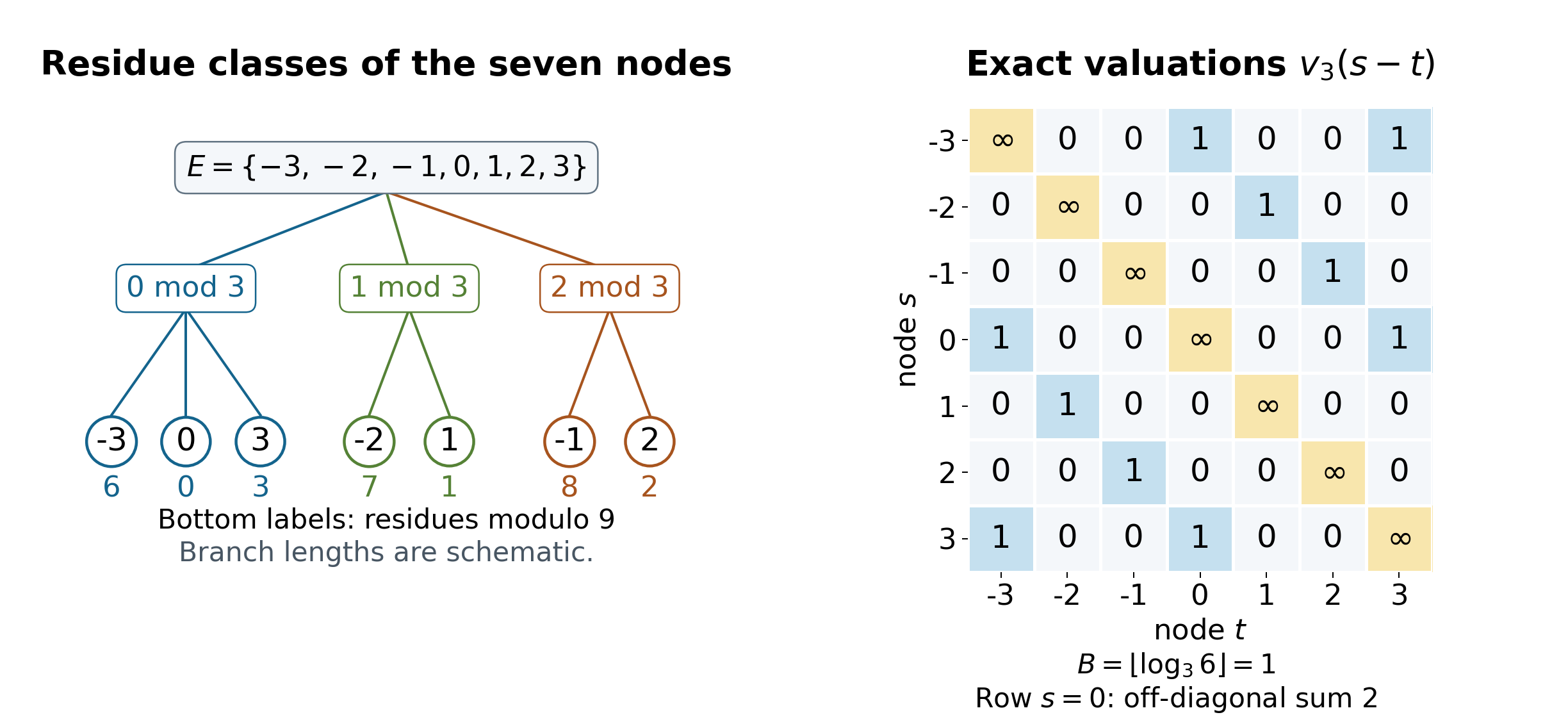
Figure 10.5. The seven nodes \(-3,\ldots,3\), grouped by their residues modulo three, and the exact matrix \(v_3(s-t)\). The diagonal is \(+\infty\). Nodes in the same indicated class have difference valuation one; all other nonzero differences have valuation zero. The groups split into singletons modulo nine. The drawing is a residue-class schematic: its line lengths are not p-adic distances. For \(R=3,p=3\), the exact separation cost in Theorem 10.34 is \(B=1\). The off-diagonal entries in the row at zero sum to two, matching \(v_3((3!)^2)=2\), but this factorial total cancels in the integral cardinal factors for the full node set. The complete mechanism is proved in (10.99)–(10.103). Human-source context: the normal-series extrapolation in Yu's freely accessible 1990 and 2013 articles, cited below. Figure program.
For an application with jet order \(M\), put \(\mu=M+1\). Replacing either logarithmic cost above by a larger maximum with a coefficient-height parameter only strengthens the hypothesis. The conclusion then follows once normality and the input jet bound (10.100) hold.
The error from projecting a logarithmic curve
Lemma 10.36 (uniform projection error). Let \(q\ne p\) be a prime, \(I\ge0\) be an integer, and use the prepared family (10.92) with integer Euler coefficients and a finite coefficient vector \(c\in\mathbb C_p^N\setminus\{0\}\). Put \(\delta=\min_j v_p(c_j)\). Take \(b\in\mathbb Z\setminus\{0\}\), \(a_i\in\mathbb Z_p\), and \(u_i,\mathcal L\in\mathbb C_p\), satisfying \(v_p(u_i)>1/(p-1)\), \(v_p(\mathcal L)\ge U\), and \(U-v_p(b)>1/(p-1)\). For \(y\in\mathbb Z_p\), define
\[ \begin{aligned} \Phi(y;\boldsymbol t)&=\mathcal Q(y;\boldsymbol t) \big|_{Y_i=\exp(yu_i)},\\ f(y;\boldsymbol t)&=\mathcal Q(y;\boldsymbol t) \big|_{Y_i=\exp(y(u_i-a_i\mathcal L/b))}. \end{aligned} \tag{10.104} \]Then for every nonnegative index \(\boldsymbol t\),
\[ v_p\bigl(f(y;\boldsymbol t)-\Phi(y;\boldsymbol t)\bigr) \ge\delta+U-v_p(b). \tag{10.105} \]Proof. Here the integer \(v(k)=\operatorname{lcm}(1,\ldots,k)\) retains its earlier meaning, distinct from the valuation \(v_p\). The prepared Taylor factor is p-integral at \(q^{-I}y+a\). Here is the slight extension of Lemma 10.28 needed for \(y\in\mathbb Z_p\): the rational polynomial \(v(k)^m\Theta(Z;k,\ell,m)\) is integral at integers. Choose an integer approximating any given p-integral argument modulo a sufficiently high power of \(p\), exceeding all its coefficient denominator valuations. Factoring the differences of monomials proves its value is p-integral, exactly as in the proof of Lemma 10.28. The Euler binomial factors are integers. Thus every prepared scalar in (10.92) is p-integral.
All displayed exponentials exist. In each monomial term the ratio of the projected exponential to the original one is \(\exp(-y\mathcal L\sum_i m_i a_i/b)\), by Proposition 9.4 in The exponential and the logarithm. Its exponent has valuation at least \(U-v_p(b)>1/(p-1)\), because \(y\), \(m_i\) and \(a_i\) are p-integral. The exact first-term exponential valuation in Proposition 9.3 of that subsection gives that the ratio minus one has valuation at least \(U-v_p(b)\). The original exponential is a local unit. Multiplying by the prepared scalar and its coefficient, then summing, proves (10.105). \(\square\)
In logarithmic applications take \(\mathcal L=p^\kappa\log\Xi\), where \(\kappa\in\mathbb Z_{\ge0}\). If \(v_p(\Xi-1)\ge U>1/(p-1)\), Proposition 9.3 gives \(v_p(\mathcal L)\ge U\). The coefficient \(a_i\) may include a denominator that is a q-power, since it remains p-integral. The precise domain and coefficient valuation cost of the projection estimate are thus visible in (10.104)–(10.105).
Normalizing the prepared series
Proposition 10.37 (a normal prepared auxiliary function). Retain the integer data of (10.92), the finite nonzero coefficient vector \(c\), and \(\delta=\min_j v_p(c_j)\). Choose a coefficient \(c_*\) of that valuation and \(\rho\in\mathbb C_p\) with \(v_p(\rho)=\theta>0\). Suppose that every logarithmic slope \(w_i\) satisfies \(v_p(w_i)>\theta+1/(p-1)\). Define \(f(y;\boldsymbol t)\) by substituting \(Y_i=\exp(yw_i)\) in (10.92), and put
\[ \begin{aligned} D&=kL,\qquad \gamma=\rho^D(k!)^L/c_*,\\ \Gamma&=v_p(\gamma)=D\theta+L v_p(k!)-\delta,\\ F(Z;\boldsymbol t)&=\gamma f(Z/\rho;\boldsymbol t). \end{aligned} \tag{10.106} \]For every nonnegative prepared index \(\boldsymbol t\), the function \(F\) is normal. At an integer node \(s\), its divided jets satisfy
\[ F_j(\rho s;\boldsymbol t)=\gamma\rho^{-j}f_j(s;\boldsymbol t),\qquad v_p(F_j(\rho s;\boldsymbol t))+j\theta=\Gamma+v_p(f_j(s;\boldsymbol t)). \tag{10.107} \]Consequently, if \(v_p(f_j(s;\boldsymbol t))\ge P\) at the node set of Theorem 10.34 for \(0\le j<\mu\), then
\[ v_p(f(x;\boldsymbol t))\ge \min\{n\mu\theta-\Gamma,\ P-((\kappa+1)\mu-1)B\} \qquad(x\in\mathbb Z_p). \tag{10.108} \]Proof. Consider one prepared polynomial factor after \(y=Z/\rho\). Its coefficient of \(Z^h\) has valuation at least \(-h\theta-\ell v_p(k!)\), and its degree is at most \(k\ell-t_0\). To see this without a coefficient estimate from another source, multiply it by \((k!)^\ell\): it is the coefficient of \(U^{t_0}\) in \[ \prod_{b=1}^k(q^{-I}Z/\rho+a+b+v(k)U)^\ell. \] All constants and \(v(k)\) are integers, while \(q\ne p\). A term of degree \(h\) in \(Z\) therefore has valuation at least \(-h\theta\). Multiplying by \(\rho^D(k!)^L\) makes every coefficient integral, because \(h\le k\ell\le D\) and \(\ell\le L\). The Euler binomial factors are integers, and \(c_j/c_*\) is locally integral. Thus the normalized polynomial part of every summand has Gauss norm at most one.
The exponential part of that summand is \(\exp(\beta Z/\rho)\), where \(\beta=\sum_i m_iw_i\). Either \(\beta=0\), or \(v_p(\beta/\rho)>1/(p-1)\), since the exponents \(m_i\) are integers. By (9.4), its coefficient of degree \(h\ge1\) has valuation \(h v_p(\beta/\rho)-v_p(h!)\ge h(v_p(\beta/\rho)-1/(p-1))+1/(p-1)>0\), tending to infinity. Its constant coefficient is one. It belongs to \(\mathcal A_1\) with norm one. The product and finite-sum statements of Lemma 9.2 now prove that \(F\in\mathcal A_1\) with norm at most one, hence is normal.
The slope hypotheses define \(f\) on the full closed disc \(|y|\le|\rho|^{-1}\), so the chain rule is valid at every integer node. It gives (10.107), also for zero jets with infinite valuation. Apply Theorem 10.34 with \(\Lambda=\Gamma+P\), then subtract \(\Gamma\), to obtain (10.108). \(\square\)
The larger scale \(D(\theta+1/(p-1))-\delta\) also suffices: (9.4) gives \(L v_p(k!)\le D/(p-1)\), and a scalar of any additional nonnegative valuation preserves normality. For the projected slopes in (10.104), it suffices that \(v_p(u_i)>\theta+1/(p-1)\) and \(U-v_p(b)>\theta+1/(p-1)\). The ultrametric inequality then supplies the slope hypotheses above. Input derivative precision remains an explicit hypothesis in (10.108), distinct from this proof of normality.
16. Prepared jets and derivative precision
The interpolation argument can keep the precision of each derivative separately. We first obtain that precision from the prepared equations, without changing the selected Euler directions.
Differentiating along the projected curve
Lemma 10.38 (the loss in an ordinary divided jet). Take the integral forms, matrix \(C\), selected column set \(J\), and derivations \(\delta_j\) of Lemma 10.23. Use those selected derivations as the \(D_j\) in (10.92), renumbering them if necessary. Let \(q\ne p\) be a prime, \(I,\nu\ge0\) be integers, and \(z_j\in\mathbb C_p\), \(1\le j<n\), satisfy \(v_p(z_j)>1/(p-1)\). Put \(\beta=v_p(b_n)\), and define
\[ \begin{aligned} w_i&=\frac1{b_nq^\nu}\sum_{j<n}C_{ij}z_j,\\ \xi_a&=\frac1{b_nq^\nu}\sum_{j<n}\lambda_{aj}z_j\quad(a\in J),\\ C_0&=\max\{v_p(v(k)),\beta\}. \end{aligned} \tag{10.109} \]Here the coefficients \(\lambda_{aj}\) are those in (10.64), with \(\lambda_{aj}=\mathbf1_{a=j}\) for selected columns. Suppose that \(v_p(w_i)>1/(p-1)\) for every \(i\). Define \(f(y;\boldsymbol t)\) by substituting \(Y_i=\exp(yw_i)\) in the prepared family (10.92). Fix \(s\in\mathbb Z_p\), an integer \(T\ge0\), and a real \(P_0\). If \(v_p(f(s;\boldsymbol t'))\ge P_0\) for every \(|\boldsymbol t'|\le T\), then
\[ v_p\bigl(f_j(s;\boldsymbol t)\bigr)\ge P_0-jC_0 \quad\text{whenever }\ |\boldsymbol t|+j\le T, \qquad f_j=\frac1{j!}\frac{d^jf}{dy^j}. \tag{10.110} \]Proof. By (10.64), \(\sum_iw_iE_i=\sum_{a\in J}\xi_a\delta_a\). Each \(\lambda_{aj}\) is p-integral, and \(q\ne p\), so either \(\xi_a=0\) or \(v_p(\xi_a)>1/(p-1)-\beta\). Differentiating along the curve therefore applies the commuting operator \(V=\partial_X+\sum_{a\in J}\xi_a\delta_a\). This identity follows directly on a term \(P(X)Y^{\boldsymbol m}\): its restriction is \(P(y)\exp(y\sum_i m_iw_i)\), whose derivative has the stated two terms. The exponential laws and convergence in Propositions 9.3–9.4 justify this differentiation on the finite prepared sum.
Write \(A=q^Iv(k)\). The additive prepared operator is \(\mathcal B_{t_0}=A^{t_0}\partial_X^{t_0}/t_0!\). For \(h\ge0\), \[ \frac{\partial_X^h}{h!}\mathcal B_{t_0} =A^{-h}\binom{t_0+h}{h}\mathcal B_{t_0+h}. \] Its scalar has valuation at least \(-h v_p(v(k))\).
For an indeterminate \(Z\), the defining product for \(\Delta\) gives \[ Z\Delta(Z;t)=(t+1)\Delta(Z;t+1)-(t+1)\Delta(Z;t). \] Repeated use of this identity expresses \(Z^h\Delta(Z;t)\) as an integer linear combination of \(\Delta(Z;e)\), with \(t\le e\le t+h\). Substitution of an Euler derivation is legitimate because all the operators commute. Multiplication by \(\xi_a^h/h!\) gives coefficients of valuation at least \(-h\beta\): for \(h>0\), (9.4) gives \(h v_p(\xi_a)-v_p(h!)\ge-h\beta\); for \(h=0\), the coefficient is one. A zero \(\xi_a\) causes no problem.
Expand \(V^j/j!\) over \(h_0+\sum_a h_a=j\). The multinomial coefficient cancels the denominator \(j!\), leaving the product of the divided powers just considered. Every resulting prepared index has total order at most \(|\boldsymbol t|+j\), and every scalar has valuation at least \(-h_0v_p(v(k))-\sum_a h_a\beta\ge-jC_0\). Evaluation at the same curve point \(s\), followed by the ultrametric inequality, proves (10.110). This proof retains the factorials; no extra \(v_p(j!)\) loss is needed. \(\square\)
Retaining the precision of each jet
Theorem 10.39 (interpolation with a linear jet loss). Retain the normal function, integer node set, \(\rho\), \(\theta\), \(n\), \(\mu\), \(B\), and \(\kappa\in\{0,1\}\) of Theorem 10.34. Suppose \(C\ge0\) and \(v_p(F_j(\rho s))+j\theta\ge\Lambda-jC\) for every node \(s\) and \(0\le j<\mu\). Then
\[ v_p(F(\rho x))\ge \min\{n\mu\theta,\ \Lambda-\kappa\mu B-(\mu-1)\max\{B,C\}\} \qquad(x\in\mathbb Z_p\subset\mathbb Q_p). \tag{10.111} \]Proof. Use the explicit Hermite remainder in the proof of Theorem 10.34. Its term with jet index \(j\) contains a coefficient of degree \(h\le\mu-1-j\) in \(A_s\). That proof gives valuations at least \(-\kappa\mu B\) for \(L_s(x)^\mu\), and at least \(-hB\) for that coefficient. The remaining power of \(x-s\) is integral. The term thus has valuation at least \(\Lambda-jC-\kappa\mu B-(\mu-1-j)B\). Since \(0\le j\le\mu-1\), \[ jC+(\mu-1-j)B\le(\mu-1)\max\{B,C\}. \] The ultrametric inequality gives the second bound in (10.111) for the full Hermite remainder. The normal quotient and its root product give the first bound \(n\mu\theta\), exactly as before. Their sum proves the claim. \(\square\)
For \(C=0\) this is Theorem 10.34. For \(C>0\), first replacing all jets by their least precision would instead give the larger loss \((\mu-1)(C+B)+\kappa\mu B\). The exact Hermite formula avoids that loss by pairing each jet with only the inverse coefficients it actually uses.
The input precision for extrapolation
Corollary 10.40 (prepared vanishing supplies the required jets). Retain the selected directions and notation of Lemma 10.38, the prepared coefficient vector \(c\ne0\), and \(\delta=\min_jv_p(c_j)\). Suppose the unprojected and projected functions \(\Phi\) and \(f\) satisfy Lemma 10.36 with \(b=b_n\), projection precision \(U\), and coefficient minimum \(\delta\). Suppose also that the slopes of \(f\) satisfy Proposition 10.37 for \(v_p(\rho)=\theta>0\). Let \(\Gamma\) be its exact scale in (10.106).
At every node of Theorem 10.34, assume \(\Phi(s;\boldsymbol t')=0\) for all \(|\boldsymbol t'|\le T\). Fix \(\boldsymbol t\) with \(|\boldsymbol t|+\mu-1\le T\), and write \(M_0=\max\{B,C_0\}\). Then, for every \(x\in\mathbb Z_p\),
\[ v_p(f(x;\boldsymbol t))\ge \min\{n\mu\theta-\Gamma,\ U+\delta-\beta -\kappa\mu B-(\mu-1)M_0\}. \tag{10.112} \]In particular the following explicit budget suffices for \(v_p(f(x;\boldsymbol t))\ge n\mu\theta-\Gamma\):
\[ U+D\theta+L v_p(k!)\ge n\mu\theta+(\kappa+1)\mu M_0, \qquad D=kL. \tag{10.113} \]Under that budget the same lower bound holds for \(\Phi(x;\boldsymbol t)\). For the full interval, \(n=2R+1\) and \(\kappa=0\); for the q-deleted interval with \(q\mid R\), \(n=2(1-1/q)R\) and \(\kappa=1\).
These hypotheses have a direct logarithmic model. Take \(z_1,\ldots,z_n\) with \(v_p(z_j)>\theta+1/(p-1)\), and put \[ u_i=q^{-\nu}\sum_{j=1}^na_{ij}z_j, \qquad \mathcal L=\sum_{j=1}^nb_jz_j, \qquad a_i=q^{-\nu}a_{in}. \] Then \(a_i\in\mathbb Z_p\), and \(w_i=u_i-a_i\mathcal L/b_n\) is exactly (10.109). If \(v_p(\mathcal L)\ge U\) and \(U-\beta>\theta+1/(p-1)\), the hypotheses of both the projection and normality estimates follow from the ultrametric inequality. The chosen-minor argument supplies the integral coefficients used for the ordinary input jets.
Proof. Vanishing of \(\Phi\) and (10.105) give \(v_p(f(s;\boldsymbol t'))\ge U+\delta-\beta\) for every required prepared index. Lemma 10.38 therefore gives the ordinary input jets with loss \(jC_0\). By (10.107), the corresponding normal jets have weighted precision \(\Gamma+U+\delta-\beta-jC_0\). Theorem 10.39 and subtraction of \(\Gamma\) prove (10.112).
Here \(\beta\le C_0\le M_0\) and \(B\le M_0\). Consequently \(\beta+\kappa\mu B+(\mu-1)M_0\le(\kappa+1)\mu M_0\). Substitute \(\Gamma+\delta=D\theta+Lv_p(k!)\) in (10.113) to see that the second entry of the minimum in (10.112) is at least the first. It also follows that \(U+\delta-\beta\ge n\mu\theta-\Gamma\). The projection error (10.105) holds at \(x\), so \(\Phi=f+(\Phi-f)\) has the same lower bound. The node counts are those proved in Corollary 10.35. \(\square\)
The coefficient minimum cancels from (10.113); it remains in the valuation conclusion through \(\Gamma\). One may instead choose the larger normalizing scale \(\Gamma'=D(\theta+1/(p-1))-\delta\) allowed by Proposition 10.37. Multiplying the normal function by a scalar of valuation \(\Gamma'-\Gamma\ge0\) repeats the proof with \(\Gamma'\) throughout. It gives the sufficient budget and its corresponding conclusion \[ U+D\left(\theta+\frac1{p-1}\right) \ge n\mu\theta+(\kappa+1)\mu M_0 \quad\Longrightarrow\quad v_p(f(x;\boldsymbol t)),\ v_p(\Phi(x;\boldsymbol t))\ge n\mu\theta-\Gamma'. \tag{10.114} \] Such a scalar exists: its required valuation is the nonnegative rational \(D/(p-1)-L v_p(k!)\), and a b-th root of \(p^a\) has valuation \(a/b\) in \(\mathbb C_p\). The conclusion with \(\Gamma'\) does not assert the stronger conclusion with \(\Gamma\).
Finally, \(v_p(v(k))=\lfloor\log_p k\rfloor\): the highest p-power dividing a least common multiple is the highest p-power dividing one of its factors, and the largest such power among \(1,\ldots,k\) is \(p^{\lfloor\log_pk\rfloor}\). Also \(\beta\le\ln|b_n|/\ln p\). Thus \(M_0\le\max\{\ln(2R),\ln k,\ln|b_n|\}/\ln p\), a useful real-valued upper bound in (10.113)–(10.114). To deduce an algebraic zero from the valuation conclusion one must additionally compare it with the height of the nonzero prepared value. Those arithmetic and numerical comparisons are separate from this interpolation argument.
17. When extrapolation forces an algebraic zero
An analytic lower bound for a valuation forces an algebraic value to vanish only when it exceeds the upper bound for a nonzero value. We prove that upper bound with the exact local degree and with the denominators of the prepared polynomial retained.
A nonzero prepared value
Use the height conventions of Section 14 and the product formula proved in Places of number fields in extensions and the product formula. The height identities for powers and inverses are proved in Heights of algebraic numbers.
Theorem 10.41 (arithmetic precision of a prepared value). Let \(K\) have degree \(d\), and let its chosen prime above \(p\) have ramification index \(e\) and residue degree \(f\). Take the prepared family (10.92) with a prime \(q\ne p\), integers \(I,J\ge0\), \(k,L\ge1\), a nonzero vector \(c\in K^N\), and integer Euler arguments \(\omega_j(\boldsymbol m)\). Let \(|m_i|\le A_i\), put \(N=kL|\mathcal M|\), \(D=kL\), and take \(x=s/q^J\), \(s\in\mathbb Z\), with \(|x|\le X\). Suppose \(\eta_i\in K^\times\) are units at the chosen prime. Evaluate (10.92) at \((x,\boldsymbol\eta)\), and call its value \(V\). Let \(|\boldsymbol t|\le T\), \(T\in\mathbb Z_{\ge0}\), and put
\[ \begin{aligned} \delta&=\min_jv_p(c_j),\qquad \Omega=\max\bigl(\{0\}\cup\{|\omega_j(\boldsymbol m)|\}\bigr),\\ \mathcal B_I(X,T)&= \left(\frac{(q^{-I}X+2k-1+v(k))^k}{k!}\right)^L \max\{1,\Omega+T\}^{T},\\ \Xi_{I,J,t_0}&= \begin{cases} 0,&I+J=0,\\ \max\{0,Lv_q(k!)+(I+J)(D-t_0)-t_0v_q(v(k))\},&I+J>0. \end{cases} \end{aligned} \tag{10.115} \]If \(V\ne0\), then
\[ \begin{aligned} v_p(V)-\delta\le\frac d{ef\ln p} \biggl(&\min\{h_\infty(c)+\ln N,\ h_2(c)+\tfrac12\ln N\}\\ &+\ln\mathcal B_I(X,T)+\Xi_{I,J,t_0}\ln q +2\sum_iA_i h(\eta_i)\biggr). \end{aligned} \tag{10.116} \]If \(t_0>D\), the value is zero automatically. The same estimate holds when the Euler arguments are any assigned integers bounded by \(\Omega\); their linear dependence on \(\boldsymbol m\) is not needed for this arithmetic assertion.
Proof. Write each row entry as its rational prepared scalar times \(\boldsymbol\eta^{\boldsymbol m}\). The additive scalar is the coefficient of \(Z^{t_0}\) in \(\Delta(q^{-I}x+a+v(k)Z;k)^\ell\). The sum of the absolute values of the coefficients of this polynomial is at most \[ \frac{\prod_{b=1}^k(q^{-I}|x|+a+b+v(k))^\ell}{(k!)^\ell} \le\left(\frac{(q^{-I}X+2k-1+v(k))^k}{k!}\right)^\ell. \] The displayed base is at least one: \(2k-1+v(k)\ge k\), and \(k^k\ge k!\). Since \(\ell\le L\), its L-th power bounds this coefficient. The product formula for \(\Delta(\omega;t_j)\) gives the remaining factor in \(\mathcal B_I\), as in Theorem 10.32. Thus every rational scalar has ordinary absolute value at most \(\mathcal B_I\).
There is no denominator away from \(q\), by Lemma 10.28 at the argument \(q^{-I-J}s+a\); the Euler factors are integers. If \(I+J=0\), every scalar is an integer. Otherwise the coefficient of degree \(h\) of the ordinary divided derivative has denominator dividing \((k!)^\ell\), because differentiating a monomial and dividing by \(t_0!\) multiplies its coefficient by an integer binomial coefficient. Its degree is at most \(k\ell-t_0\). Evaluation at \(q^{-I-J}s+a\) costs at most \((I+J)(k\ell-t_0)\) in q-adic valuation. Multiplication by \(v(k)^{t_0}\) restores \(t_0v_q(v(k))\). Taking \(\ell\le L\) gives the clearing factor \(q^{\Xi_{I,J,t_0}}\). If \(t_0>D\), every additive derivative is zero.
Choose a coefficient \(c_*\) of valuation \(\delta\), and put \(z=V/c_*\). At the chosen prime the maximum norm of the coefficient vector \(c/c_*\) is exactly one. For \(V\ne0\), the product formula therefore gives \[ ef\ln p\,(v_p(V)-\delta) =-\ln|z|_{\mathfrak p} =\sum_{v\ne\mathfrak p}\ln|z|_v. \] The factor is \(ef\), since \(|z|_{\mathfrak p}=p^{-f\operatorname{ord}_{\mathfrak p}(z)}\) and \(\operatorname{ord}_{\mathfrak p}=ev_p\).
At each archimedean embedding, the triangle inequality bounds the sum by \(N\) times the coefficient maximum times the entry maximum. Alternatively Cauchy–Schwarz gives the coefficient Euclidean norm times \(\sqrt N\) times the entry maximum. This last inequality follows by applying \((\sum u_jv_j)^2\le(\sum u_j^2)(\sum v_j^2)\) to the absolute values; its difference is \(\sum_{i<j}(u_iv_j-u_jv_i)^2\ge0\). At finite places the ultrametric inequality uses maximum norms and introduces no factor \(N\).
Sum these bounds outside the chosen prime. The normalized coefficient norms contribute exactly \(d h_\infty(c)\), or \(d h_2(c)\), because their missing finite norm is one. There are \(d\) archimedean embeddings with a complex pair counted twice. The rational scalar contributes at most \(d\ln\mathcal B_I\) there. Its clearing factor contributes at most \(d\Xi_{I,J,t_0}\ln q\) over the primes above \(q\), by the local-degree identity for the element \(q\).
At every other place, the torus contribution is bounded by \(\sum_iA_i\ln\max\{|\eta_i|_v,|\eta_i|_v^{-1}\}\). Its omitted contribution at the chosen prime is zero, since the \(\eta_i\) are units. Summing over all places gives \(2d\sum_iA_i h(\eta_i)\), by the inverse-height identity and product formula. Divide by \(ef\ln p\), and take the better of the two coefficient norm bounds, to obtain (10.116). Every step used only integrality and the absolute size of the Euler factors, proving the final assertion too. \(\square\)
Fractional nodes and the coefficient field
Proposition 10.42 (roots and a common local unit). Let \(\vartheta_i\in K^\times\) be units at \(p\), and choose \(q^J\)-th roots \(\eta_i\) in a fixed algebraic embedding into \(\mathbb C_p\). Put \(F=K(\eta_1,\ldots,\eta_r)\). For \(x=s/q^J\), consider the prepared value with torus coordinates \(\eta_i^s\). Theorem 10.41 applies over \(F\). Its torus height term is at most \(2X\sum_iA_i h(\vartheta_i)\) when \(|x|\le X\), but its local-degree coefficient is
\[ \frac{[F:\mathbb Q]}{e_Ff_F} =\frac d{ef}\frac{[F:K]}{[F_{\mathfrak P}:K_{\mathfrak p}]}. \tag{10.117} \]One cannot replace this coefficient by \(d/(ef)\) without further information.
If every exponent belongs to \(\boldsymbol m_*+q^J\mathbb Z^r\), where \(\boldsymbol m_*\) is one of the exponent vectors, define \(\widehat A_i=\max_{\boldsymbol m}|m_i-m_{*,i}|\le2A_i\). Then the common-factor identity is
\[ \begin{aligned} V&=\boldsymbol\eta^{s\boldsymbol m_*}V_0,\\ V_0&=\sum_{\boldsymbol m,a,\ell} c_{\boldsymbol m,a,\ell}\,\mathcal S_{\boldsymbol m,a,\ell}(x;\boldsymbol t) \boldsymbol\vartheta^{s(\boldsymbol m-\boldsymbol m_*)/q^J}\in K, \qquad v_p(V)=v_p(V_0). \end{aligned} \tag{10.118} \]Here \(\mathcal S\) denotes the rational prepared scalar in (10.92). In this case (10.116) may instead use \(d/(ef)\) and the torus height term \(2X\sum_i\widehat A_i h(\vartheta_i)\), with the same \(\mathcal B_I\), clearing factor, and coefficient heights. For a logarithmic curve with \(\vartheta_i=\exp(u_i)\), choose \(\eta_i=\exp(u_i/q^J)\). The exponential laws of Proposition 9.4 give \(\eta_i^{q^J}=\vartheta_i\) and \(\exp(xu_i)=\eta_i^s\), identifying the fractional analytic value with the stated algebraic value.
Proof. A root of a local unit is a local unit. The height power identity gives \(h(\eta_i)=h(\vartheta_i)/q^J\), and hence \(h(\eta_i^s)=|x|h(\vartheta_i)\). Heights of the coefficient vector are unchanged by extending the field: every archimedean embedding is repeated \([F:K]\) times, and the corresponding finite-place contribution is multiplied by that same factor, as proved by the local-degree identities in the earlier places lesson. Dividing by the field degree cancels that factor. The relative ramification and residue degrees multiply the original ones, and their product is \([F_{\mathfrak P}:K_{\mathfrak p}]\). This proves (10.117) and the assertion about applying the preceding theorem.
In the coset case, \((\boldsymbol m-\boldsymbol m_*)/q^J\) is an integer vector. Factoring its common root monomial gives (10.118), term by term. The common factor is a local unit, so it changes no valuation. Apply the last assertion of Theorem 10.41 to \(V_0\): the Euler arguments stay their original integers, and the new exponent bound is \(\widehat A_i/q^J\). The torus coordinates are \(\vartheta_i^s\), of height \(|s|h(\vartheta_i)\). Their contribution is at most \(2|s|\sum_i(\widehat A_i/q^J)h(\vartheta_i)\le2X\sum_i\widehat A_i h(\vartheta_i)\). The rational scalars and coefficient vector have not changed. \(\square\)
The two comparisons in Theorem 10.43 exclude every finite valuation in the case illustrated in Figure 10.6.
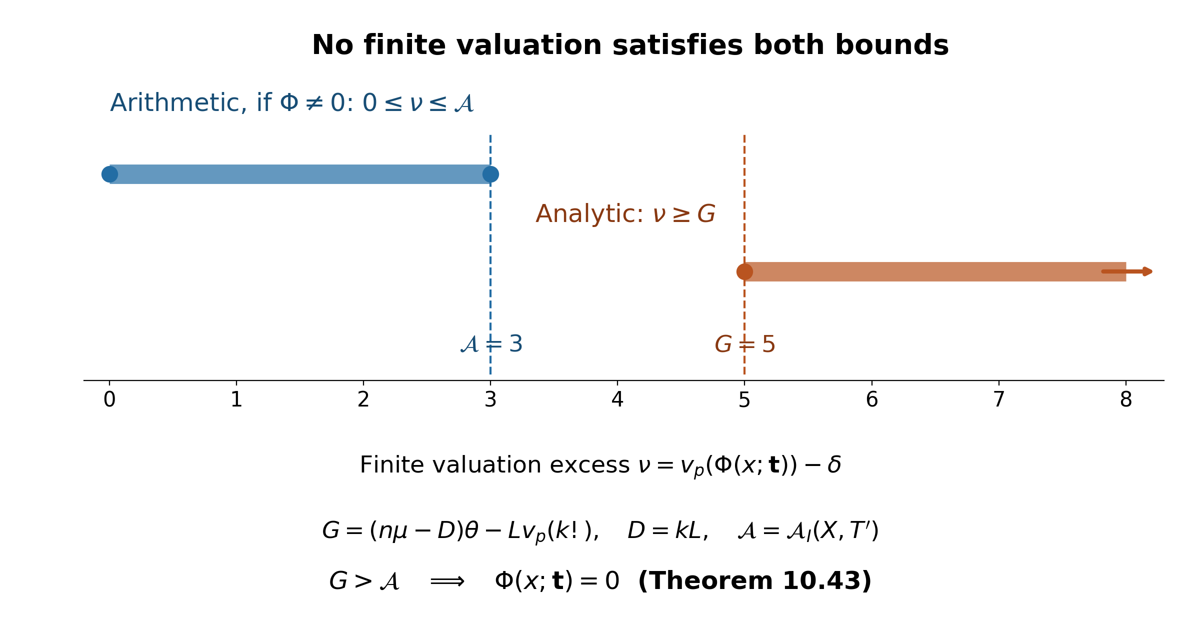
Figure 10.6. The prepared scalars are p-integral and the torus coordinates are local units, so \(\Phi/c_*\) is p-integral and the valuation excess \(\nu=v_p(\Phi(x;\boldsymbol t))-\delta\) is nonnegative. If the value is nonzero, the product-formula proof of Theorem 10.41 gives \(\nu\le\mathcal A_I(X,T')\). The analytic proof gives \(\nu\ge(n\mu-D)\theta-Lv_p(k!)\). The drawn endpoints \(\mathcal A=3,G=5\) illustrate these two intervals; they are not parameters of a specified auxiliary function. Their separation is exactly the strict second comparison in (10.120), and forces \(\Phi(x;\boldsymbol t)=0\). The zero value has infinite valuation and is outside the finite axis. Human-source context: the product-formula step in Yu's free2013 article, cited below. Figure program.
An explicit zero-forcing step
Theorem 10.43 (extension of the prepared zeros). Retain the hypotheses of Corollary 10.40 over the field \(K\), and suppose that at every integer \(x\) the unprojected function is the algebraic prepared value at \((x,\vartheta_1^x,\ldots,\vartheta_r^x)\), with \(\vartheta_i\in K^\times\) local units. Let \(T'=T-\mu+1\ge0\), and let \(X\ge0\) be real. Put
\[ \begin{aligned} Q_I&=\begin{cases}0,&I=0,\\L(kI+v_q(k!)),&I>0,\end{cases}\\ \mathcal A_I(X,T')&=\frac d{ef\ln p}\biggl( \min\{h_\infty(c)+\ln N,\ h_2(c)+\tfrac12\ln N\}\\ &\hspace{28mm}+\ln\mathcal B_I(X,T')+Q_I\ln q +2X\sum_iA_i h(\vartheta_i)\biggr). \end{aligned} \tag{10.119} \]The node count \(n\), \(\kappa\), \(\theta\), and \(M_0=\max\{B,C_0\}\) are those of Corollary 10.40. If
\[ \begin{aligned} U+D\theta+L v_p(k!)&\ge n\mu\theta+(\kappa+1)\mu M_0,\\ (n\mu-D)\theta-L v_p(k!)&>\mathcal A_I(X,T'), \end{aligned} \tag{10.120} \]then \(\Phi(x;\boldsymbol t)=0\) for every integer \(|x|\le X\) and every \(|\boldsymbol t|\le T'\). With the larger normalizing scale of (10.114), an alternative sufficient pair is
\[ \begin{aligned} U+D\left(\theta+\frac1{p-1}\right)&\ge n\mu\theta+(\kappa+1)\mu M_0,\\ (n\mu-D)\theta-\frac D{p-1}&>\mathcal A_I(X,T'). \end{aligned} \tag{10.121} \]Proof. The first line of (10.120) supplies the analytic budget of Corollary 10.40. At every stated index its conclusion gives \[ v_p(\Phi(x;\boldsymbol t))-\delta \ge(n\mu-D)\theta-L v_p(k!). \] If the prepared value were nonzero, Theorem 10.41 with \(J=0\) would give the opposite upper bound \(\mathcal A_I(X,T')\): its torus coordinates have height \(|x|h(\vartheta_i)\), and its clearing exponent is at most \(Q_I\). The strict second line of (10.120) contradicts this. A prepared index with \(t_0>D\) already has zero value. These cases prove every claimed zero. The same argument using (10.114) instead proves (10.121). \(\square\)
Both comparisons remove \(\delta\), so they are invariant under scaling the coefficient vector. The first comparison gives enough analytic precision; the second makes a nonzero algebraic value impossible. At fractional nodes one must additionally use the field or common-factor rule of Proposition 10.42. Applying this step repeatedly requires checking these inequalities, the slope conditions, and the available derivative orders at every stage.
18. Retaining the derivative orders in the height budget
The uniform estimate (10.115) bounds every coefficient by the sum of all coefficients. It also discards the factorials in the Euler binomials. Those bounds suffice for Theorem 10.43, but a numerical induction benefits from retaining the actual derivative order. We now do so, including the average over the symmetric initial nodes. The additive estimate below has the form of Lemma 1.6 in Yu's free 1990 paper; we give its full proof using only an elementary factorial inequality.
Positive polynomial majorants
Let \(\Omega_j=\max_{\boldsymbol m\in\mathcal M}|\omega_j(\boldsymbol m)|\), for \(1\le j<r\), and let \(\Omega_\Sigma=\sum_{j<r}\Omega_j\). For integers \(\Omega,h\ge0\), define \(E_h(\Omega)=\binom{\Omega+h}{h}\). Thus \(E_0(\Omega)=E_h(0)=1\). Put \(\Gamma_0=1\); for \(h>0\), put \(\Gamma_h=0\) if \(r=1\), and \(\Gamma_h=\binom{\Omega_\Sigma+r-2+h}{h}\) if \(r\ge2\). Use empty products and sums when \(r=1\). Define the positive polynomial
\[ \begin{aligned} \mathcal P_{I,X}(Z) &=\left(\frac1{k!}\prod_{b=1}^k (q^{-I}X+k-1+b+v(k)Z)\right)^L\\ &=\sum_{u=0}^{D}\mathcal C_{I,u}(X)Z^u, \qquad D=kL. \end{aligned} \tag{10.122} \]Theorem 10.44 (an order-dependent scalar bound). For the rational prepared scalar \(\mathcal S_{\boldsymbol m,a,\ell}(x;\boldsymbol t)\) in (10.92), with \(0\le a<k\), \(1\le\ell\le L\), \(|x|\le X\), and \(t_0\le D\), one has
\[ \begin{aligned} |\mathcal S_{\boldsymbol m,a,\ell}(x;\boldsymbol t)| &\le\mathcal H_I(X;\boldsymbol t) :=\mathcal C_{I,t_0}(X)\prod_{j<r}E_{t_j}(\Omega_j),\\ \mathcal B_I^*(X,T) &:=\max_{|\boldsymbol t|\le T,\ t_0\le D} \mathcal H_I(X;\boldsymbol t). \end{aligned} \tag{10.123} \]An index with \(t_0>D\) has zero scalar. If \(\Omega_j=0\), its Euler factor is \(\Delta(0;t_j)=1\), so changing that index to zero leaves the scalar unchanged. The maximum in (10.123) is at least one and satisfies
\[ \begin{aligned} \mathcal B_I^*(X,T)&\le\mathcal B_I(X,T),\\ \mathcal B_I^*(X,T)&\le \left(\mathrm e\left(2+\frac{q^{-I}X}{k}\right)\right)^D \max_{\substack{u,h\ge0\text{ integers}\\u\le D,\ u+h\le T}} v(k)^u\Gamma_h. \end{aligned} \tag{10.124} \]Here \(\mathcal B_I\) is (10.115); the second bound retains the division of the total order between the additive and Euler directions. For \(h>0\), one may further bound \(\Gamma_h\) by \([\mathrm e(1+(\Omega_\Sigma+r-1)/h)]^h\).
Proof. At a given real or complex \(x\), replace each factor \(q^{-I}x+a+b\) by its absolute-value upper bound \(q^{-I}X+a+b\). Expansion of the product bounds the absolute value of each coefficient by the corresponding coefficient of this polynomial with nonnegative coefficients. Its constant coefficient after division by \(k!\) is at least one: each factor \(q^{-I}X+a+b\) is at least \(b\). Consequently increasing its power from \(\ell\) to \(L\) can only increase every coefficient. Increasing \(a\) to \(k-1\) has the same property. Taking the coefficient of \(Z^{t_0}\) gives \(\mathcal C_{I,t_0}(X)\).
For an integer \(\omega\) with \(|\omega|\le\Omega\), the product defining \(\Delta(\omega;t)\) gives \(|\Delta(\omega;t)|\le E_t(\Omega)\). Indeed \(|\omega+b|\le\Omega+b\), for \(1\le b\le t\), and the factorial \(t!\) is retained. When \(\Omega=0\), the Euler argument is zero and every such binomial is one. This proves (10.123), the degree-zero case and the duplicate-direction assertion. Every \(\mathcal C_{I,u}(X)\) is positive. At \(X=0\), it is the prepared Taylor coefficient at the integer \(k-1\), so it is an integer by Lemma 10.28 and is at least one. The coefficients increase with \(X\). In particular the index \(\boldsymbol t=0\) proves \(\mathcal B_I^*\ge1\).
For the first inequality in (10.124), each \(\mathcal C_{I,u}(X)\) is at most \(\mathcal P_{I,X}(1)\). Bounding each of its \(k\) factors by \(q^{-I}X+2k-1+v(k)\) gives the additive part of (10.115). Put \(\Omega=\max_j\Omega_j\), with \(\Omega=0\) for an empty index set. The Euler product is at most \(\max\{1,\Omega+T\}^T\), as in Theorem 10.32. Hence this sharper maximum never exceeds the earlier one.
We prove the additive estimate used for the second inequality. For every integer \(k\ge1\), monotonicity of \(\log x\) on each interval \([j-1,j]\) gives \(\log k!\ge\int_1^k\log x\,dx=k\log k-k+1\). Thus \(k!\ge\mathrm e(k/\mathrm e)^k\), including \(k=1\). At \(y\ge0\), coefficient comparison with \((Z+k)^{k\ell}/(k!)^\ell\) gives \[ \begin{aligned} |\Theta(z;k,\ell,u)| &\le\frac{\binom{k\ell}{u}(|z|+k)^{k\ell-u}}{(k!)^\ell}\\ &\le\frac{\ell^u}{u!}\, \frac{(|z|+k)^{k\ell}}{(k!)^\ell} \le\left(\frac{\mathrm e(|z|+k)}k\right)^{k\ell}. \end{aligned} \tag{10.125} \] The first comparison takes absolute values in the differentiated product. The second uses \(\binom{k\ell}{u}\le(k\ell)^u/u!\) and \(|z|+k\ge k\). The last uses the factorial bound and \(\ell^u/u!\le\mathrm e^\ell\), since this is one nonnegative term of the exponential series. Derivatives above degree \(k\ell\) are zero. Apply (10.125) with \(z=q^{-I}x+a\), multiply by \(v(k)^u\), and increase \(\ell\) to \(L\). The base \(\mathrm e(2+q^{-I}X/k)\) is greater than one. The same bound applies to \(\mathcal C_{I,u}(X)\), by using \(x=X,a=k-1,\ell=L\).
Finally, \(E_h(\Omega)\) is the coefficient of \(Z^h\) in the product of \(\Omega+1\) copies of \(1+Z+Z^2+\cdots\). Distributing \(h\) objects among these slots gives \(\binom{\Omega+h}{h}\). Multiplying these series over the Euler directions uses \(\Omega_\Sigma+r-1\) slots, so every fixed Euler product of total order \(h\) is at most \(\Gamma_h\): it is one of the nonnegative summands of that coefficient. For no Euler directions only order zero occurs. This proves the second inequality in (10.124). When \(h>0,r\ge2\), the numerator product for \(\Gamma_h\) is at most \((\Omega_\Sigma+r-1+h)^h\); the factorial bound gives the further estimate. When \(r=1\), its left side is zero. \(\square\)
Averaging the initial rows
Keep the data of Theorem 10.32, and write \(H=\sum_i A_i h(\vartheta_i)\). Let \(r_0\) be the number of Euler indices with \(\Omega_j>0\). The representative prepared indices after removing duplicate zero directions, and their row count, are
\[ \begin{aligned} \mathcal J_T&=\{\boldsymbol t\ge0:|\boldsymbol t|\le T,\ t_0\le D, \ t_j=0\text{ if }\Omega_j=0\},\\ J_T&=|\mathcal J_T|= \sum_{u=0}^{\min(D,T)}\binom{T-u+r_0}{r_0}, \qquad M_*=(2S+1)J_T. \end{aligned} \tag{10.126} \]Corollary 10.45 (a sharper initial coefficient budget). If \(N>M_*\), the integral kernel in Theorem 10.32 exists with every originally specified zero and with
\[ \begin{aligned} h_\infty(c)\le h_2(c)\le&\ \tfrac12\log N+ \frac{\log|\Delta_K|}{2d}\\ &+\frac1{N-M_*}\sum_{s=-S}^S\sum_{\boldsymbol t\in\mathcal J_T} \left(\tfrac12\log N+ \log\mathcal H_0(|s|;\boldsymbol t)+2|s|H\right). \end{aligned} \tag{10.127} \]A simpler consequence is
\[ \begin{aligned} h_2(c)\le&\ \tfrac12\log N+\frac{\log|\Delta_K|}{2d}\\ &+\frac{M_*}{N-M_*} \left(\tfrac12\log N+\log\mathcal B_0^*(S,T) +\frac{2S(S+1)}{2S+1}H\right). \end{aligned} \tag{10.128} \]When \(N>M\) in Theorem 10.32, the right side of (10.128) is no larger than the right side of (10.96).
Proof. An index above the additive degree has zero scalar. An index in a zero Euler direction duplicates the row with that index set to zero, by Theorem 10.44. Removing it therefore preserves every original vanishing condition. Fixing \(t_0=u\) leaves \(r_0\) Euler indices of total order at most \(T-u\). The divider argument from Theorem 10.32 counts them as \(\binom{T-u+r_0}{r_0}\), also when \(r_0=0\). This proves (10.126).
At each retained row \((s,\boldsymbol t)\), the same adelic row-norm proof as in Theorem 10.32 now uses \(\mathcal H_0(|s|;\boldsymbol t)\). At finite places the prepared scalars are still integers. The row norm is therefore at most \(\sqrt N\mathcal H_0(|s|;\boldsymbol t)\exp(2|s|H)\). The scalar majorant is at least one: its positive additive coefficient at integer \(|s|+k-1\) is an integer by Lemma 10.28, and every retained Euler factor is a positive integer. Hence the displayed row bound is at least one, as required by the maximum in (8.40). A row that vanishes for additional reasons has norm zero and contributes the factor one there. Apply that proved weighted Siegel lemma with all weights one, retaining the separate row factors. Its logarithm is exactly (10.127), and its finite conditions give algebraic-integer coordinates. Dependent rows are already included in that lemma.
The uniform scalar bound in (10.123) and the identity \(\sum_{s=-S}^S|s|=S(S+1)\) give (10.128). Finally \(M_*\le M\), \(\mathcal B_0^*\le\mathcal B\), and \(S(S+1)/(2S+1)\le S\). All summands are nonnegative. The function \(m/(N-m)\) increases for \(0\le m<N\), as cross multiplication shows. These facts prove the comparison with (10.96). The nonzero polynomial and its required ordinary jets follow from Proposition 10.31, exactly as before. \(\square\)
The smaller nonzero-value budget
For the integer target nodes in Theorem 10.43, define, at each \(\boldsymbol t\in\mathcal J_{T'}\),
\[ \begin{aligned} \mathcal A_{I,\boldsymbol t}^*(X)=\frac d{ef\ln p}\biggl(& \min\{h_\infty(c)+\ln N,h_2(c)+\tfrac12\ln N\}\\ &+\ln\mathcal H_I(X;\boldsymbol t) +\Xi_{I,0,t_0}\ln q+2XH\biggr),\\ \mathcal A_I^*(X,T')&=\max_{\boldsymbol t\in\mathcal J_{T'}} \mathcal A_{I,\boldsymbol t}^*(X). \end{aligned} \tag{10.129} \]Corollary 10.46 (zero forcing with the retained orders). Under the hypotheses of Theorem 10.43, its first analytic comparison and
\[ (n\mu-D)\theta-Lv_p(k!)>\mathcal A_I^*(X,T') \tag{10.130} \]force every zero asserted there. The analogous assertion holds with its larger normalizing scale and lower bound \((n\mu-D)\theta-D/(p-1)\). Moreover \(\mathcal A_I^*(X,T')\le\mathcal A_I(X,T')\).
Proof. Repeating the product-formula proof of Theorem 10.41 uses the individual scalar bound \(\mathcal H_I(X;\boldsymbol t)\) instead of \(\mathcal B_I\), with its same exact clearing exponent. Thus a nonzero value at a retained index has valuation excess at most \(\mathcal A_{I,\boldsymbol t}^*\). The analytic lower bound contradicts (10.130). Every removed index either has zero scalar by additive degree or duplicates a retained index by setting its zero Euler directions to zero. The larger normalizing scale gives the stated second conclusion by the same argument. Finally \(\mathcal H_I(X;\boldsymbol t)\le\mathcal B_I(X,T')\) and \(\Xi_{I,0,t_0}\le Q_I\). Taking the maximum proves the comparison with (10.119). Fractional targets still require the field or common-factor conditions of Proposition 10.42. \(\square\)
These refinements retain the exact factorials, lcm, derivative orders and mean node size. To obtain a numerical logarithm estimate, their bounds and the analytic slope and order conditions must all be checked for its chosen induction parameters.
19. Passing to one exponent coset
The next auxiliary function is obtained by retaining one coset of the exponent set and dividing its exponent differences by \(q\). Two facts justify this step: independent root monomials separate the cosets, and an invertible affine change preserves the filtered Euler jets. The saturated Kummer theorem and the Newton reparametrization have already been proved in Theorem 10.14 and Lemma 10.30. We now combine them, retaining the coefficient field and the condition on the integer node. This is the algebraic mechanism of the coset passage in Yu's free 2013 paper, Lemma 5.4.
Separating the root monomials
Theorem 10.47 (exact coset extraction). Let \(F\) be a characteristic-zero field, \(q\) a prime, and \(\vartheta_i\in F^\times\), \(1\le i\le r\). Choose \(\eta_i^q=\vartheta_i\), and suppose \([F(\eta_1,\ldots,\eta_r):F]=q^r\). Take a finite set \(\mathcal M\subset\mathbb Z^r\), coefficients \(A_{\boldsymbol m}\in F\), and an integer \(s\) coprime to \(q\). If \(\sum_{\boldsymbol m}A_{\boldsymbol m}\boldsymbol\eta^{s\boldsymbol m}=0\), then for each residue vector \(\boldsymbol\rho\in\{0,\ldots,q-1\}^r\),
\[ \sum_{\boldsymbol m\equiv\boldsymbol\rho\ (q)} A_{\boldsymbol m}\boldsymbol\vartheta^{s(\boldsymbol m-\boldsymbol\rho)/q}=0. \tag{10.131} \]Proof. The \(q^r\) monomials \(\boldsymbol\eta^{\boldsymbol\rho}\) span the root field over \(F\): reduce every exponent modulo \(q\), using \(\eta_i^q=\vartheta_i\ne0\), also for negative exponents. The span is closed under multiplication. Every nonzero element of this finite-dimensional span has an inverse in it: multiplication by that element is injective in the surrounding field and thus surjective on the span. Hence it is the whole root field. Its degree is \(q^r\), so these spanning monomials are a basis.
Group the given sum by \(\boldsymbol\rho\). Its coefficient after factoring \(\boldsymbol\eta^{s\boldsymbol\rho}\) is exactly the expression in (10.131), an element of \(F\). Let \(\boldsymbol\rho'\) be the least nonnegative residues of \(s\boldsymbol\rho\), and put \(\boldsymbol b=(s\boldsymbol\rho-\boldsymbol\rho')/q\). Then \(\boldsymbol\eta^{s\boldsymbol\rho}=\boldsymbol\vartheta^{\boldsymbol b}\boldsymbol\eta^{\boldsymbol\rho'}\). Multiplication by \(s\) permutes the residue vectors because \(q\nmid s\). Thus grouping gives a relation among distinct basis monomials, with each grouped coefficient multiplied by the nonzero scalar \(\boldsymbol\vartheta^{\boldsymbol b}\). Every coefficient vanishes, proving (10.131). \(\square\)
This argument extracts exact zeros. A large finite valuation of the sum does not by itself supply that valuation for each coset.
The next prepared family
Theorem 10.48 (coset restriction and affine jet transfer). Take a number field \(K\), a prime \(q\ne p\), local units \(\vartheta_i\in K^\times\), and the integer Euler forms \(\omega_j(\boldsymbol m)=\sum_iC_{ij}m_i\) in (10.92). Let \(c\in K^N\setminus\{0\}\). Suppose that a field \(F\supset K\) and chosen roots \(\eta_i^q=\vartheta_i\) satisfy the degree condition of Theorem 10.47. Let \(\mathcal E\) be any set of integers coprime to \(q\). Assume that all original prepared values at \((s/q,\eta_1^s,\ldots,\eta_r^s)\), \(s\in\mathcal E\), vanish through total order \(T\).
Choose \(\boldsymbol m_*\) at which some coefficient attains \(\delta=\min v_p(c_j)\). Retain its exponent coset, and put
\[ \begin{aligned} \mathcal M'&=\{(\boldsymbol m-\boldsymbol m_*)/q: \boldsymbol m\in\mathcal M,\ \boldsymbol m\equiv\boldsymbol m_*\ (q)\},\\ c'_{\boldsymbol n,a,\ell}&=c_{\boldsymbol m_*+q\boldsymbol n,a,\ell},\\ Q'(X,Y)&=\sum_{\boldsymbol n,a,\ell}c'_{\boldsymbol n,a,\ell} \Delta(q^{-(I+1)}X+a;k)^\ell Y^{\boldsymbol n}. \end{aligned} \tag{10.132} \]Then \(Q'\ne0\). Its new prepared family, with stage \(I+1\) and the same Euler matrix \(C\), vanishes at \((s,\boldsymbol\vartheta^s)\), \(s\in\mathcal E\), through the same total order \(T\).
The original prepared values restricted to this coset and the new prepared values are related by the affine changes
\[ \begin{aligned} \Delta(qZ+\omega_j(\boldsymbol m_*);t_j) &=\sum_{u_j=0}^{t_j}d_{t_j,u_j}^{(j)}\Delta(Z;u_j), \qquad d_{t_j,t_j}^{(j)}=q^{t_j},\\ \min_{|\boldsymbol t|\le T}v_p(\text{original coset value at }s/q) &=\min_{|\boldsymbol t|\le T}v_p(\text{new prepared value at }s). \end{aligned} \tag{10.133} \]The minimum identity includes \(\infty\) when all values are zero. The coefficients satisfy
\[ \min v_p(c'_j)=\delta,\qquad h_\infty(c')\le h_\infty(c),\qquad h_2(c')\le h_2(c). \tag{10.134} \]Global integrality of \(c\) is retained by \(c'\). For any convex body \(\mathcal C\) and vector \(x_0\) with \(\mathcal M\subset q^{-I}\mathcal C-x_0\), one has
\[ \begin{aligned} \mathcal M'&\subset q^{-(I+1)}\mathcal C-(x_0+\boldsymbol m_*)/q,\\ \deg_{Y_i}(\text{ordinary monomial shift of }Q') &\le\left\lfloor \frac{\max_{\boldsymbol m\in\mathcal M}m_i- \min_{\boldsymbol m\in\mathcal M}m_i}{q}\right\rfloor. \end{aligned} \tag{10.135} \]Its additive degree is at most \(D=kL\).
Proof. Fix \(s\in\mathcal E\) and a prepared index. The rational additive and Euler factors, multiplied by the coefficients \(c\), belong to \(K\subset F\). Theorem 10.47 therefore extracts a zero separately in every exponent coset. For the chosen one, factoring \(\boldsymbol\eta^{s\boldsymbol m_*}\) gives a zero with torus monomials \(\boldsymbol\vartheta^{s\boldsymbol n}\).
The additive scalar at \(s/q\) is exactly \(v(k)^{t_0}\Theta(q^{-(I+1)}s+a;k,\ell,t_0)\). The old Euler argument is \(\omega_j(\boldsymbol m_*+q\boldsymbol n)= q\omega_j(\boldsymbol n)+\omega_j(\boldsymbol m_*)\). Lemma 10.30 gives the first line of (10.133), and both its matrix and inverse have coefficients in \(\mathbb Z[1/q]\). The product changes only to indices with \(u_j\le t_j\), keeping \(t_0\) fixed. On the finite space of indices of total order at most \(T\), it is triangular with nonzero diagonal \(q^{\sum_{j<r}t_j}\); its inverse preserves the same filtration. Every new jet is therefore a linear combination of the extracted old coset jets, proving all the claimed zeros without reducing \(T\).
The factored root monomial is a local unit, since every \(\vartheta_i\) is one. The affine matrix and inverse are p-integral because \(q\ne p\). Applying the ultrametric inequality to each change shows in both directions that the minimum valuation cannot decrease. This proves the second line of (10.133). It compares the jets of an individual coset; extraction from the whole sum used exact vanishing.
The selected coefficient vector is nonzero and contains a coefficient of the original minimum valuation. This proves the first assertion of (10.134). At every place its maximum norm is at most the old one; at each archimedean embedding the same is true for its Euclidean norm. Summing logarithms in the projective height definitions proves the remaining two inequalities. Coordinates of an integral vector remain integral. Distinct exponents give distinct \(\boldsymbol n\), so Lemma 10.29 proves \(Q'\ne0\), as in Proposition 10.31.
For the geometric inclusion, divide \(\boldsymbol m+x_0\in q^{-I}\mathcal C\) by \(q\) and subtract \((x_0+\boldsymbol m_*)/q\). Each coordinate width of the retained exponent set is divided by \(q\). Multiplying \(Q'\) by the inverse of its coordinatewise least Laurent monomial makes its torus exponents nonnegative, with exactly those widths. They are integers, proving (10.135). The additive degree is unchanged. \(\square\)
Figure 10.7 shows the exponent change in Theorem 10.48 for a square support at \(q=2\).
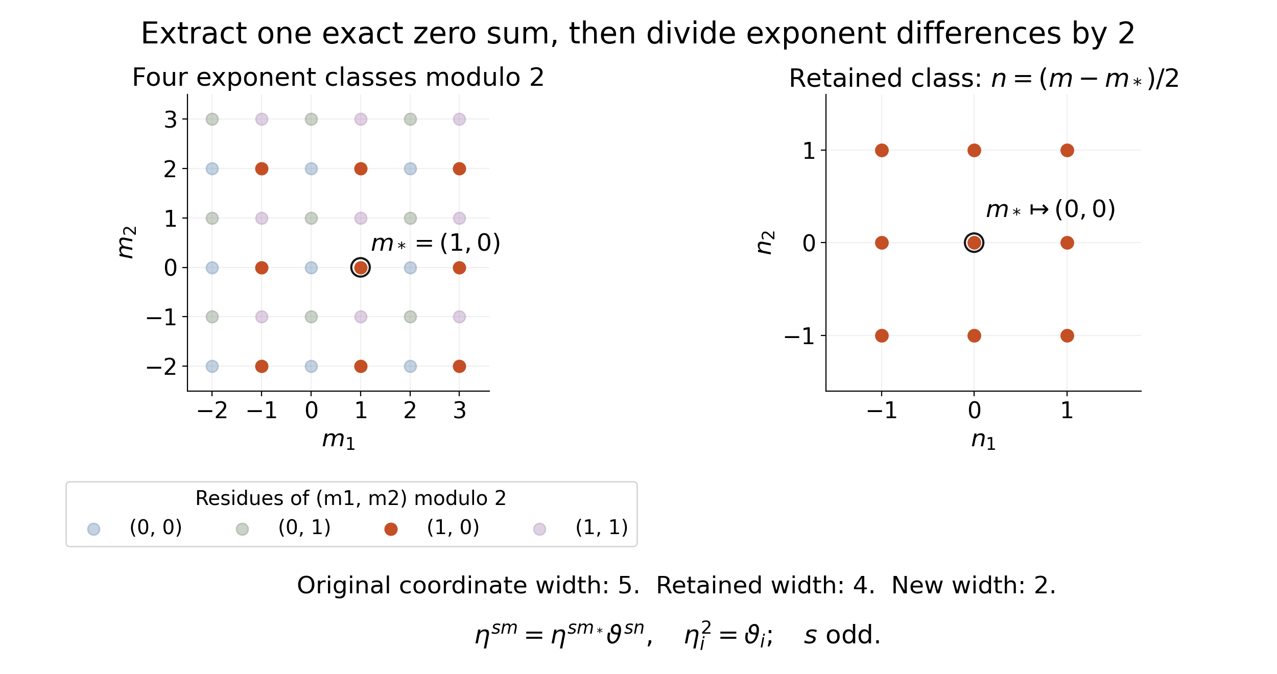
Figure 10.7. The exact support is \(\mathcal M=\{-2,-1,0,1,2,3\}^2\). The four colors mark its four classes modulo two. Selecting \(\boldsymbol m_*=(1,0)\) retains the nine orange points \(m_1\in\{-1,1,3\},m_2\in\{-2,0,2\}\); translating by \(-\boldsymbol m_*\) and dividing by two gives \(\{-1,0,1\}^2\). The original coordinate width five becomes retained width four and then new width two, exactly as in (10.135). For odd \(s\), full root-field degree separates the four root monomials in Theorem 10.47; their exact zero sums can then be treated separately. In the selected class the common local unit is \(\boldsymbol\eta^{s\boldsymbol m_*}\), and the remaining monomials are \(\boldsymbol\vartheta^{s\boldsymbol n}\), by (10.132)–(10.133). The displayed support illustrates that algebraic transformation; it does not assert a particular coefficient vector or numerical logarithm bound. Human-source context: Yu's free2013 Lemma5.4, cited below. Figure program.
Root-of-unity phases and the coefficient field
Corollary 10.49 (q-primary phases). Let \(\alpha_0,\theta_1,\ldots,\theta_r\) be the saturated generators of Theorem 10.14. Choose \(\xi^q=\alpha_0\) and \(\rho_i^q=\theta_i\), and put \(F=K(\xi)\). For an integer \(P\ge1\) coprime to \(q\) and integers \(d_i\), set
\[ \vartheta_i=\theta_i^P\alpha_0^{d_i},\qquad \eta_i=\rho_i^P\xi^{d_i},\qquad [F(\boldsymbol\eta):F]=q^r,\qquad h(\vartheta_i)=P h(\theta_i). \tag{10.136} \]Thus Theorems 10.47–10.48 apply to these phased torus coordinates. If the \(\theta_i\) are local units and \(q\ne p\), all the displayed roots are local units. In particular one may take \(P=p^a\), \(a\ge0\).
Proof. Theorem 10.14 gives total root degree \(q^{r+1}\), and the same proved Kummer argument for \(\alpha_0\) alone gives \([F:K]=q\). Hence \([F(\boldsymbol\rho):F]=q^r\). Clearly \(F(\boldsymbol\eta)\subset F(\boldsymbol\rho)\). Choose integers \(A,B\) with \(AP+Bq=1\); integer division gives such a pair because \(P\) and \(q\) are coprime. Then \(\rho_i=(\eta_i\xi^{-d_i})^A\theta_i^B\), giving the reverse inclusion and the degree in (10.136). The q-th power identity follows directly. A root of unity has height zero; applying the product-height inequality in both directions shows that multiplying by it preserves height. The proved power identity then gives \(h(\vartheta_i)=P h(\theta_i)\). Finally taking valuations in the defining power equations proves every unit assertion. \(\square\)
The coefficient field \(F\) holds the root-of-unity phase, while the selected new coefficients and torus bases in Theorem 10.48 remain in \(K\). The next zero set consists of the stated integer nodes coprime to \(q\); extension to further nodes uses the extrapolation results, with their slope and precision conditions.
20. Retaining the phase congruence in the next support
The phase used to make a local unit close to one need not belong to the global field \(K\). A support congruence controls its powers. After division by \(q\), the congruence has either one class or \(q\) classes; in the latter case the q-primary root separates them. We prove both cases, keeping all the new coefficients in \(K\). This supplies the phase and support passage of Yu's free 2013 paper, equations (5.51)–(5.61), before the separate analytic extension to further nodes.
The congruence and its phase classes
Lemma 10.50 (division of a phase congruence). Let \(q\) be prime, \(G_0\ge1\) an integer, and \(a\in\mathbb Z\). The congruence \(qu+a\equiv0\pmod{G_0}\) has the following solutions:
\[ \begin{aligned} u&\equiv-q^{-1}a\pmod{G_0}, &&\gcd(q,G_0)=1,\\ u&\equiv-a/q+bG_0/q\pmod{G_0}, \quad 0\le b<q, &&q\mid G_0,\ q\mid a. \end{aligned} \tag{10.137} \]In the second case there is no solution if \(q\nmid a\), and the displayed \(q\) classes are distinct. Suppose additionally that \(\alpha_0\in K^\times\) is not a q-th power, \(\mu_q\subset K\), and \(\beta^q=\alpha_0\). Then, for every integer \(s\) prime to \(q\), the \(q\) powers \(\beta^{sb}\), \(0\le b<q\), are linearly independent over \(K\).
Proof. If \(q\) and \(G_0\) are coprime, integer division gives integers \(A,B\) with \(Aq+BG_0=1\). Multiplication by \(A\) solves the congruence, uniquely modulo \(G_0\). If \(q\mid G_0\), reduction modulo \(q\) first forces \(q\mid a\). Put \(H=G_0/q\). The original congruence is equivalent to \(u+a/q\equiv0\pmod H\), so \(u=-a/q+bH+G_0v\) for a unique \(b\) modulo \(q\). This proves the second formula and its distinctness.
The complete Kummer argument of Theorem 10.14 applied to the one independent class \(\alpha_0\) proves \([K(\beta):K]=q\). Equivalently \(1,\beta,\ldots,\beta^{q-1}\) are a basis, since their span is the field and has that degree, as proved in Theorem 10.47. Multiplication by \(s\) permutes exponents modulo \(q\); reducing \(\beta^{sb}\) by \(\beta^q=\alpha_0\) multiplies those basis elements by nonzero scalars in \(K\). This proves the asserted independence, also for negative \(s\). \(\square\)
The phased prepared values
Take the saturated generators \(\alpha_0,\theta_1,\ldots,\theta_r\) of Theorem 10.14, with \(\alpha_0\) of order \(q^u\). Let \(G_0\ge1\), put \(G=q^uG_0\), and choose roots of unity and algebraic roots in a fixed embedding such that
\[ \begin{aligned} \zeta^{G_0}&=\alpha_0,\quad \zeta\text{ has order }G,\quad \xi^q=\zeta,\quad \beta=\xi^{G_0},\quad \beta^q=\alpha_0,\\ \rho_i^q&=\theta_i,\qquad \gamma_i=\theta_i^P\zeta^{d_i},\qquad \eta_i=\rho_i^P\xi^{d_i},\qquad \eta_i^q=\gamma_i , \end{aligned} \tag{10.138} \]where \(P\ge1\) is prime to \(q\), and \(d_i\in\mathbb Z\). The existence of \(\zeta\) with the specified order is a hypothesis here; Lemma 10.53 constructs it for the local residue modulus. Write \(d\cdot m=\sum_i d_i m_i\), and let \(F=K(\beta)\). Theorem 10.14 gives \([F(\boldsymbol\rho):F]=q^r\).
Let \(I\ge0,k,L\ge1,T\ge0\) be integers. Let a finite nonempty \(\Lambda\subset\mathbb Z^r\) satisfy \(d\cdot\iota\equiv\varepsilon\pmod{G_0}\). Fix \(\iota_0\in\Lambda\), an integer Euler matrix \(C\), and a nonzero coefficient vector \(c\in K^N\), with \(N=kL|\Lambda|\). The fractional prepared values are
\[ \begin{aligned} \Psi(s/q;\boldsymbol t)= \sum_{\iota,a,\ell}c_{\iota,a,\ell} v(k)^{t_0}\Theta(q^{-(I+1)}s+a;k,\ell,t_0) \prod_{j<r}\Delta(C_j(\iota-\iota_0);t_j) \boldsymbol\eta^{s(\iota-\iota_0)} . \end{aligned} \tag{10.139} \]Here \(C_j(m)=\sum_i C_{ij}m_i\), the indices \(a,\ell\) retain \(0\le a<k,1\le\ell\le L\), and the sum ranges over \(\iota\in\Lambda\).
Theorem 10.51 (complete phase and support passage). Suppose that (10.139) is zero for every \(s\) in a set \(\mathcal E\subset\mathbb Z\) prime to \(q\), and every \(|\boldsymbol t|\le T\). Put \(\delta=\min_jv_p(c_j)\), where \(q\ne p\) and the \(\theta_i\) are units in a fixed embedding into \(\mathbb C_p\).
Choose \(\iota_{\min}\) at which some coefficient has valuation \(\delta\), and let \(\lambda_*\in\{0,\ldots,q-1\}^r\) represent \(\iota_{\min}-\iota_0\) modulo \(q\). First retain the exponents in this q-coset, and write
\[ \iota-\iota_0=q\lambda+\lambda_*, \qquad a_*=d\cdot\lambda_*, \qquad q\,d\cdot\lambda+a_*\equiv0\pmod{G_0}. \tag{10.140} \]If \(\gcd(q,G_0)=1\), retain this whole coset and put \(\varepsilon'=-q^{-1}a_*\pmod{G_0}\). If \(q\mid G_0\), then \(q\mid a_*\). Put \(H=G_0/q\), \(a_0=-a_*/q\), and choose the unique \(b_{\min}\in\{0,\ldots,q-1\}\) for which the \(\lambda\) corresponding to \(\iota_{\min}\) satisfies \(d\cdot\lambda\equiv a_0+b_{\min}H\pmod{G_0}\). Retain only that subclass and put \(\varepsilon'=a_0+b_{\min}H\).
The resulting nonempty set \(\Lambda'\) has \(d\cdot\lambda\equiv\varepsilon'\pmod{G_0}\). Select \(\lambda_0\in\Lambda'\) corresponding to \(\iota_{\min}\), retain the same coefficients \(c'_{\lambda,a,\ell}=c_{\iota,a,\ell}\), and form
\[ \begin{aligned} Q'(X,Y)&=\sum_{\lambda,a,\ell}c'_{\lambda,a,\ell} \Delta(q^{-(I+1)}X+a;k)^\ell Y^{\lambda-\lambda_0},\\ \Psi'(s;\boldsymbol t)&= \sum_{\lambda,a,\ell}c'_{\lambda,a,\ell} v(k)^{t_0}\Theta(q^{-(I+1)}s+a;k,\ell,t_0) \prod_{j<r}\Delta(C_j(\lambda-\lambda_0);t_j) \boldsymbol\gamma^{s(\lambda-\lambda_0)} . \end{aligned} \tag{10.141} \]Then \(Q'\ne0\), and \(\Psi'(s;\boldsymbol t)=0\) for every \(s\in\mathcal E,|\boldsymbol t|\le T\). All those values belong to \(K\), although the individual \(\gamma_i\) need not belong to \(K\). The coefficients retain global integrality when present, satisfy \(\min v_p(c'_j)=\delta\), and have \(h_\infty(c')\le h_\infty(c)\), \(h_2(c')\le h_2(c)\).
If \(\Lambda\subset q^{-I}\mathcal C-x\), the uncentered support satisfies
\[ \begin{aligned} \Lambda'&\subset q^{-(I+1)}\mathcal C-x', \qquad x'=(x+\iota_0+\lambda_*)/q,\\ \deg_{Y_i}(\text{ordinary monomial shift of }Q') &\le \left\lfloor\frac{\max_{\iota\in\Lambda}\iota_i- \min_{\iota\in\Lambda}\iota_i}{q}\right\rfloor, \qquad \deg_XQ'\le kL . \end{aligned} \tag{10.142} \]Proof. Since \(d\cdot(\iota-\iota_0)\) is divisible by \(G_0\), let \(w_\iota=d\cdot(\iota-\iota_0)/G_0\in\mathbb Z\). The torus part of an old fractional term is \(\boldsymbol\rho^{Ps(\iota-\iota_0)}\beta^{s w_\iota}\). The latter factor belongs to \(F\), while its rational prepared scalar and coefficient belong to \(K\). Over \(F\), the monomials \(\boldsymbol\rho^{Ps\lambda_*}\), one for each q-residue vector, are independent: \([F(\boldsymbol\rho):F]=q^r\) and \(Ps\) is prime to \(q\), so Theorem 10.47 supplies exactly that basis permutation. Thus every original zero separates into a zero for each first q-coset.
In the selected coset, substituting (10.140) into the zero and removing the common nonzero factor \(\boldsymbol\rho^{Ps\lambda_*}\xi^{s a_*}\) gives \[ \sum_{\iota\text{ in the selected coset},a,\ell} c_{\iota,a,\ell}\mathcal S_\iota(s;\boldsymbol t) \boldsymbol\gamma^{s\lambda}=0, \] where \(\mathcal S_\iota\) contains the additive scalar and the original Euler arguments. This equality holds for every specified \(s,\boldsymbol t\). Lemma 10.50 proves that the divided support has exactly the stated phase congruence when \(q\) and \(G_0\) are coprime.
Suppose \(q\mid G_0\). Lemma 10.50 gives the \(q\) subclasses \(d\cdot\lambda=a_0+bH+G_0v_\lambda\). Since \(q\mid G_0\), (10.138) implies \(\zeta^H=\xi^{qH}=\beta\). Multiply the last zero by \(\zeta^{-s a_0}\). The contribution of subclass \(b\) now belongs to \(\beta^{sb}K\): each term is its coefficient and rational scalar times \(\boldsymbol\theta^{Ps\lambda}\alpha_0^{s v_\lambda}\beta^{sb}\). The \(q\) powers \(\beta^{sb}\) are independent by Lemma 10.50, so every subclass sum is zero. In particular the subclass containing \(\iota_{\min}\) is zero for all the specified indices, not just at one node.
Remove the common local unit \(\boldsymbol\gamma^{s\lambda_0}\). The old Euler arguments are \[ C_j(\iota-\iota_0)= qC_j(\lambda-\lambda_0)+C_j(q\lambda_0+\lambda_*). \] The shift is an integer. Applying the invertible affine binomial change of Lemma 10.30 in every Euler direction converts the extracted zeros into the new ones in (10.141). Both changes preserve the total-order cutoff, as proved in Theorem 10.48. The additive scalar is already the stage \(I+1\) scalar and is unchanged.
For \(\lambda\in\Lambda'\), the integer \(v'_\lambda=d\cdot(\lambda-\lambda_0)/G_0\) exists. Each new torus term is \(\boldsymbol\theta^{Ps(\lambda-\lambda_0)}\alpha_0^{s v'_\lambda}\in K\). This proves the coefficient-field assertion. All roots of unity are local units, since their finite powers are one; roots of the local units \(\theta_i\) are units too. Thus every removed common torus factor is a local unit. The coefficient subset contains a coefficient of valuation \(\delta\); the projective-height and integrality assertions follow from the proved subset inequalities in Theorem 10.48. Distinct new exponents and the binomial basis in Lemma 10.29 give \(Q'\ne0\).
Finally divide \(\iota+x\in q^{-I}\mathcal C\) by \(q\) and use \(\iota=\iota_0+\lambda_*+q\lambda\) to obtain the inclusion in (10.142). Centering at \(\lambda_0\) changes no coordinate width. Every retained width is at most the original width divided by \(q\), and is an integer. The monomial shift and additive bound follow as in Theorem 10.48. \(\square\)
Figure 10.8 gives the exact two-class split in the case \(q\mid G_0\).
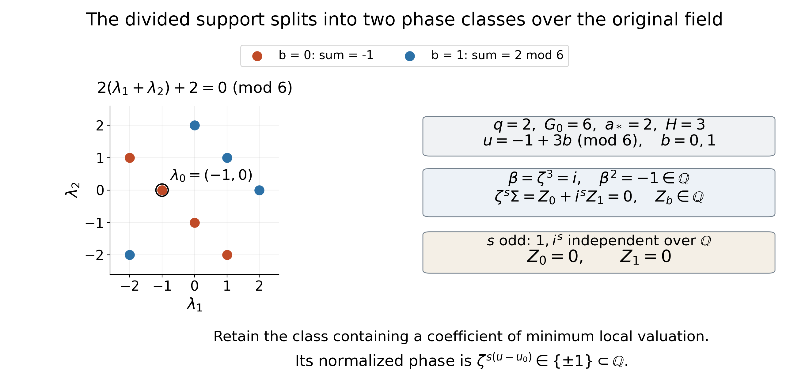
Figure 10.8. Here \(q=2,G_0=6,d=(1,1)\), and the first residue vector is \(\lambda_*=(1,1)\), so \(a_*=2\). The divided support is the eight points \(\lambda\in\{-2,-1,0,1,2\}^2\) with \(2(\lambda_1+\lambda_2)+2\equiv0\pmod6\). The original support may be taken as \(\{(0,0)\}\cup\{2\lambda+(1,1)\}\), with reference \(\iota_0=(0,0)\); every original point has coordinate sum divisible by six. Put \(K=\mathbb Q,\alpha_0=-1\), choose a primitive twelfth root \(\zeta\) with \(\zeta^6=-1\), and write \(\beta=\zeta^3=i\) in a complex embedding. The normalized phase sum at a fixed odd node is \(Z_0+i^sZ_1\), with each \(Z_b\in\mathbb Q\). When that sum is zero, independence in Lemma 10.50 forces both coefficient sums to vanish. Red points have coordinate sum \(-1\), blue points have sum \(-4\) or \(2\). The circled reference \(\lambda_0=(-1,0)\) illustrates retaining the subclass containing a coefficient of minimum valuation; its normalized phase is one. Choosing a blue reference instead gives phases in \(\{\pm1\}\), also in \(\mathbb Q\). These are exactly the congruence, extraction and field-return mechanisms of Theorem 10.51 and (10.140)–(10.142). The plotted coefficient sums are formal variables. Human-source context: Yu's free2013 equations5.51–5.59, cited below. Figure program.
The analytic branch and arithmetic height
Corollary 10.52 (the phase does not enlarge the height field). If \(v_p(\gamma_i-1)>1/(p-1)\), choose the fractional branch
\[ \eta_i=\exp\bigl(q^{-1}\log\gamma_i\bigr),\qquad \rho_i^q=\theta_i,\qquad \rho_i^P\xi^{d_i}=\eta_i . \tag{10.143} \]Such a choice of the \(\rho_i\) exists. It identifies (10.139) with the fractional values of the corresponding logarithmic curve. At an integer node \(|s|\le X\), a nonzero new value in (10.141) satisfies
\[ \begin{aligned} v_p(\Psi'(s;\boldsymbol t))-\delta \le\frac{[K:\mathbb Q]}{ef\ln p}\biggl(& \min\{h_\infty(c')+\ln N',h_2(c')+\tfrac12\ln N'\}\\ &+\ln\mathcal H_{I+1}(X;\boldsymbol t) +\Xi_{I+1,0,t_0}\ln q +2PX\sum_i A'_i h(\theta_i)\biggr), \end{aligned} \tag{10.144} \]where \(N'=kL|\Lambda'|\), \(A'_i=\max_{\lambda\in\Lambda'}|\lambda_i-\lambda_{0,i}|\), and \(\mathcal H\) uses the new integer Euler arguments in Theorem 10.44. An index above the additive degree is already zero. Every local degree in (10.144) is that of \(K\), not the degree of a field containing all individual phases.
Proof. The exponential laws proved in Proposition 9.4 give the q-th power of the chosen \(\eta_i\) as \(\gamma_i\), since \(q\ne p\) changes no slope valuation. Begin with any root \(\rho_i^q=\theta_i\). The quotient \(\eta_i/(\rho_i^P\xi^{d_i})\) is in \(\mu_q\). Raising to \(P\) permutes that cyclic group because \(q\nmid P\); multiplication of \(\rho_i\) by the appropriate q-th root of unity therefore gives (10.143). This proves the branch identification without a further root-existence assertion.
Theorem 10.51 writes each new torus term over \(K\) as a power of \(\alpha_0\) times powers of the \(\theta_i\). At every place, a root of unity has absolute value one, because its order-th power is one. Thus these phases contribute zero to every local norm bound, including the chosen p-adic place. The prepared scalar has the order-dependent archimedean bound \(\mathcal H_{I+1}\) and the rational clearing factor of Theorem 10.41. Apply its complete normalized product-formula argument over \(K\), retaining the coefficient norms and using \(|Ps(\lambda_i-\lambda_{0,i})|\le PX A'_i\). The signed torus-height sum is \(2[K:\mathbb Q]PX\sum_i A'_ih(\theta_i)\). This proves (10.144). \(\square\)
Constructing the local phase
Lemma 10.53 (lifting the residue phase and its depth). Let \(K_{\mathfrak p}\) be the completion at the chosen prime above \(p\), with ramification index \(e\) and residue field of order \(p^f\). Suppose \(q\ne p\), and let \(\alpha_0\in K\) have order \(q^u\), \(u\ge1\). Then \(q^u\mid G=p^f-1\), and there is a primitive G-th root \(\zeta\in K_{\mathfrak p}\) such that
\[ G_0=G/q^u,\qquad \zeta^{G_0}=\alpha_0,\qquad \theta_i\zeta^{-r_i}\equiv1\pmod{\mathfrak p} \tag{10.145} \]for suitable integers \(r_i\), whenever the \(\theta_i\in K^\times\) are local units. Given a real depth target \(\vartheta\ge0\), let \(t\) be the least nonnegative integer with \(p^t>e/(p-1)\). Choose an integer \(j\ge0\) with \(p^t/e+j>\vartheta+1/(p-1)\), put \(h=t+j\), and set
\[ \begin{aligned} P&=p^h,\qquad d_i=-Pr_i,\qquad \gamma_i=\theta_i^P\zeta^{d_i},\\ v_p(\gamma_i-1)&\ge p^t/e+j> \vartheta+\frac1{p-1}. \end{aligned} \tag{10.146} \]Thus these phases supply the required analytic branch and supernormal slope depth. This is a sufficient explicit choice of \(P\); using a smaller prescribed \(P\) in a numerical estimate requires checking its depth separately.
Proof. We first prove the lifting assertion directly. In a complete discretely valued field, take a polynomial \(f\) with integral coefficients and an integral \(x_0\) satisfying \(v_p(f(x_0))>0\), \(v_p(f'(x_0))=0\). Define \(x_{n+1}=x_n-f(x_n)/f'(x_n)\). A finite polynomial expansion gives \(f(x+y)=f(x)+f'(x)y+y^2R(x,y)\) with \(R\) integral when \(x,y\) are integral. The linear terms cancel at the Newton step, so \(v_p(f(x_{n+1}))\ge2v_p(f(x_n))\). Also \(f'(x_{n+1})-f'(x_n)\) has positive valuation, leaving the derivative a unit. Every step remains integral and in the original residue class. The successive differences have valuations tending to infinity, hence form a Cauchy sequence. Completeness gives its limit, and the polynomial difference identity proves that the limit is a root. If \(x,y\) are roots in that residue class, then \(0=f(y)-f(x)=(y-x)(f'(x)+(y-x)R(x,y))\). The factor in parentheses is a unit. Therefore \(x=y\). This proves existence and uniqueness of a simple-residue lift, including the case of a zero residual error where the iteration has already stopped.
Apply this to \(X^m-1\), for \(p\nmid m\). Its derivative at a unit is a unit. In particular a prime-to-\(p\) root of unity reducing to one is one, by uniqueness in that residue class. Reduction is consequently injective on all prime-to-\(p\) roots of unity. The reduction of \(\alpha_0\) has its exact order \(q^u\): a smaller order would make a nontrivial prime-to-\(p\) root reduce to one. Since the finite multiplicative residue group has order \(G\), we get \(q^u\mid G\).
The group of G-th roots in \(K_{\mathfrak p}\) maps bijectively to that residue group: every nonzero residue solves \(X^G-1\) and has its unique lift. Multiplication commutes with reduction, and the finite-field cyclicity proved in Section 1 therefore gives a primitive root \(z\). Write \(\alpha_0=z^{G_0a}\) with \(q\nmid a\), since its order is \(q^u\). Let \(n=G/q^{v_q(G)}\), so \(\gcd(n,q)=1\). Choose \(a'\equiv a\pmod{q^u}\) and \(a'\equiv1\pmod n\): Bezout's identity gives a solution by varying \(a'\) among \(a+q^u b\). Then \(\gcd(a',G)=1\). The primitive root \(\zeta=z^{a'}\) has \(\zeta^{G_0}=\alpha_0\). Its reduction generates the residue group, so every \(\overline{\theta_i}\) is \(\overline\zeta^{\,r_i}\). This proves (10.145).
Put \(g_i=\theta_i\zeta^{-r_i}\). Its positive valuation distance from one is at least \(1/e\), unless it is already one. The proved p-power inequality of Lesson 9 is \[ v_p(g_i^{p^{a+1}}-1)\ge \min\{p\,v_p(g_i^{p^a}-1),\,v_p(g_i^{p^a}-1)+1\}. \] The function on the right increases with its argument. For \(0\le a<t\), the lower bound \(p^a/e\) is at most \(1/(p-1)\), by the definition of \(t\). Induction therefore gives \(v_p(g_i^{p^t}-1)\ge p^t/e>1/(p-1)\). Each further p-power adds one by the exact power law already proved in Lesson 9; if a power is one its infinite valuation satisfies the same bound. After \(j\) further steps we obtain (10.146), because \(g_i^P=\gamma_i\). Finally \(P\) is prime to \(q\), so all the root-field and phase arguments above apply. Proposition 9.4 gives \(v_p(\log\gamma_i)=v_p(\gamma_i-1)\), including the infinite value when \(\gamma_i=1\); hence these logarithmic slopes have the stated depth. \(\square\)
Filling the missing integer nodes
Theorem 10.51 gives the new zeros at nodes prime to \(q\). We can now prove a precise condition for filling the remaining nodes, while keeping the height comparison over \(K\).
Corollary 10.54 (phase-sensitive q-deleted-node closure). Take the new family (10.141), with \(\gamma_i=\exp(u_i)\), and retain the slope, projection and selected integer Euler-basis hypotheses of Corollary 10.40 at stage \(I+1\). In particular \(v_p(w_i)>\theta+1/(p-1)\), \(v_p(\mathcal L)\ge U\), and \(U-v_p(b_n)>\theta+1/(p-1)\). Let \(R\ge1,\mu\ge1,T\ge0\) be integers with \(T'=T-\mu+1\ge0\). Suppose that \(\Psi'(s;\boldsymbol t)=0\) for every \(s\in[-R,R]\cap\mathbb Z\) prime to \(q\) and every \(|\boldsymbol t|\le T\). Put \(n=2R-2\lfloor R/q\rfloor\), \(B=\lfloor\log_p(2R)\rfloor\), \(C_0=\max\{v_p(v(k)),v_p(b_n)\}\), \(M_0=\max\{B,C_0\}\), and \(D=kL\). For \(X\ge0\), define the nonzero-value budget
\[ \begin{aligned} \mathcal A_{\mathrm{ph}}(X,T')= \max_{\substack{|\boldsymbol t|\le T'\\t_0\le D}} \frac{[K:\mathbb Q]}{ef\ln p}\biggl(& \min\{h_\infty(c')+\ln N',h_2(c')+\tfrac12\ln N'\}\\ &+\ln\mathcal H_{I+1}(X;\boldsymbol t) +\Xi_{I+1,0,t_0}\ln q +2PX\sum_iA'_ih(\theta_i)\biggr). \end{aligned} \tag{10.147} \]If
\[ \begin{aligned} U+D\theta+Lv_p(k!)&\ge n\mu\theta+2\mu M_0,\\ (n\mu-D)\theta-Lv_p(k!)&>\mathcal A_{\mathrm{ph}}(X,T'), \end{aligned} \tag{10.148} \]then \(\Psi'(x;\boldsymbol t)=0\) for every integer \(|x|\le X\) and every \(|\boldsymbol t|\le T'\). In particular \(X=R\) fills all the previously omitted integer nodes in the interval. With the larger normalizing scale, the alternative sufficient pair is
\[ \begin{aligned} U+D\left(\theta+\frac1{p-1}\right)&\ge n\mu\theta+2\mu M_0,\\ (n\mu-D)\theta-\frac D{p-1}&>\mathcal A_{\mathrm{ph}}(X,T'). \end{aligned} \tag{10.149} \]If \(q\mid R\), the node count is exactly \(n=2(1-1/q)R\). For a desired order \(0\le O\le T\), the choice \(\mu=T-O+1\) makes the output order exactly \(T'=O\).
Proof. The q-deleted input set has the stated exact count and separation cost \(\kappa=1\), by Corollary 10.35. The complete analytic proof of Corollary 10.40 at the new stage applies to the local torus coordinates \(\gamma_i\). Its normality, prepared integrality, ordinary input jets and projection estimates use those local units and their logarithmic slopes; they do not require each \(\gamma_i\) to lie in \(K\). The first line of (10.148) is its exact sufficient precision budget, with \(\kappa+1=2\). Consequently \[ v_p(\Psi'(x;\boldsymbol t))-\delta \ge(n\mu-D)\theta-Lv_p(k!) \] at every stated integer and derivative index.
The support congruence in Theorem 10.51 does put each of these integer values in \(K\). If a value were nonzero, Corollary 10.52 would bound its valuation excess above by the corresponding summand of (10.147), and hence by \(\mathcal A_{\mathrm{ph}}\). The second line of (10.148) is a strict contradiction. An index with \(t_0>D\) is already zero. This proves the full conclusion. Using the larger scale and its proved lower bound (10.114) instead proves (10.149); the two scales have their respective conclusions. Finally \(q\mid R\) gives \(\lfloor R/q\rfloor=R/q\), and the asserted order choice is the identity \(T-(T-O+1)+1=O\). \(\square\)
The phase and support passage, the local phase construction and the conditional closure of the missing nodes now have complete proofs. A numerical Yu estimate still requires a verified coefficient construction and a check of the slope, order and strict height comparisons at every stage with its actual parameters.
21. Constructing coefficients for the phased values
The initial coefficient construction can also be performed over \(K\) when the separate phased torus bases lie outside \(K\). What matters is the field of each normalized row entry. The support congruence determines that field and removes the root-of-unity phase from every absolute-value estimate.
Theorem 10.55 (an initial kernel over the original field). Let \(K\) have degree \(d\) and discriminant \(\Delta_K\). Take nonzero \(\theta_i\in K\), a root of unity \(\alpha_0\in K\), an integer \(G_0\ge1\), and a root of unity \(\zeta\) with \(\zeta^{G_0}=\alpha_0\). Let \(P\in\mathbb Z_{\ge1}\), \(d_i\in\mathbb Z\), and set \(\gamma_i=\theta_i^P\zeta^{d_i}\). The separate \(\gamma_i\) need not lie in \(K\).
Take integers \(r,k,L\ge1\), \(S,T\ge0\), and a nonempty finite set \(\Lambda\subset\mathbb Z^r\) of distinct vectors satisfying \(\boldsymbol d\cdot\lambda\equiv\varepsilon\pmod{G_0}\), where \(\boldsymbol d=(d_1,\ldots,d_r)\). Fix \(\lambda_0\in\Lambda\), put \(A_i=\max_{\lambda\in\Lambda}|\lambda_i-\lambda_{0i}|\), and take integer Euler forms \(\omega_j(\lambda)=C_j(\lambda-\lambda_0)\), \(1\le j<r\). Write \(D=kL\), \(N=kL|\Lambda|\), and use \(\mathcal J_T,J_T,M_*=(2S+1)J_T\) from (10.126), with these new Euler arguments. Define \(H_{\mathrm{ph}}=P\sum_iA_i h(\theta_i)\).
If \(N>M_*\), there is a nonzero vector \(c\in\mathcal O_K^N\) for which
\[ \begin{aligned} Q(X,Y)&=\sum_{\lambda,a,\ell}c_{\lambda,a,\ell} \Delta(X+a;k)^\ell Y^{\lambda-\lambda_0},\\ \Psi_0(s;\boldsymbol t)&=\sum_{\lambda,a,\ell}c_{\lambda,a,\ell} v(k)^{t_0}\Theta(s+a;k,\ell,t_0) \prod_{j<r}\Delta(\omega_j(\lambda);t_j) \gamma^{s(\lambda-\lambda_0)} =0 \end{aligned} \tag{10.150} \]for every integer \(|s|\le S\) and every \(|\boldsymbol t|\le T\), with \(0\le a<k\), \(1\le\ell\le L\). The Laurent polynomial \(Q\) is nonzero. Every normalized monomial in these equations belongs to \(K\), since
\[ v_\lambda=\frac{\boldsymbol d\cdot(\lambda-\lambda_0)}{G_0}\in\mathbb Z, \qquad \gamma^{s(\lambda-\lambda_0)} =\alpha_0^{s v_\lambda} \prod_i\theta_i^{Ps(\lambda_i-\lambda_{0i})}\in K. \tag{10.151} \]The vector may be chosen with the separate-row budget
\[ \begin{aligned} h_\infty(c)\le h_2(c)\le& \tfrac12\ln N+\frac{\ln|\Delta_K|}{2d}\\ &+\frac1{N-M_*} \sum_{s=-S}^S\sum_{\boldsymbol t\in\mathcal J_T} \left(\tfrac12\ln N+ \ln\mathcal H_0(|s|;\boldsymbol t)+2|s|H_{\mathrm{ph}}\right), \end{aligned} \tag{10.152} \]and hence with the mean-node budget
\[ \begin{aligned} h_2(c)\le& \tfrac12\ln N+\frac{\ln|\Delta_K|}{2d}\\ &+\frac{M_*}{N-M_*} \left(\tfrac12\ln N+\ln\mathcal B_0^*(S,T) +\frac{2S(S+1)}{2S+1}H_{\mathrm{ph}}\right). \end{aligned} \tag{10.153} \]These estimates involve \(K\) and the original \(\theta_i\), even when the individual phases require a larger global field.
Proof. Subtracting the two support congruences gives the integer \(v_\lambda\). Raising \(\zeta^{G_0}=\alpha_0\) to \(s v_\lambda\) proves (10.151), for negative \(s\) and negative exponent differences as well. This identity puts every matrix entry of (10.150) in \(K\).
The prepared scalar in each entry is an integer: Lemma 10.28 proves the additive assertion at every integer \(s+a\), and each rising Euler binomial at an integer is an integer. An index with \(t_0>D\) has zero row. If \(\omega_j\) vanishes throughout the support, its factor is \(\Delta(0;t_j)=1\); setting \(t_j=0\) gives the same row and a no larger total order. Thus imposing the representative rows imposes every stated equation. Counting them exactly as in (10.126) gives \(M_*\) rows and \(N\) columns, including any further zero or dependent rows.
We bound each representative row over \(K\). At an archimedean embedding its Euclidean norm is at most \[ \sqrt N\,\mathcal H_0(|s|;\boldsymbol t) \prod_i\max\{|\sigma(\theta_i)|,|\sigma(\theta_i)|^{-1}\}^{P|s|A_i}. \] At a finite place its maximum norm is at most the analogous product without the first two factors. Indeed the scalar is an integer, while the root of unity \(\alpha_0^{s v_\lambda}\) in (10.151) has absolute value one at every place. Theorem 10.44 supplies the scalar bound. The product formula, with the height conventions of Section 14, gives the exact identity \[ \frac1d\sum_v\ln\max\{|\theta_i|_v,|\theta_i|_v^{-1}\} =2h(\theta_i). \] Consequently the logarithm of the row-norm bound is \(\tfrac12\ln N+\ln\mathcal H_0(|s|;\boldsymbol t)+2|s|H_{\mathrm{ph}}\). This bound is nonnegative, since its scalar majorant is at least one by Theorem 10.44. A zero row has the allowed row factor one.
Apply the complete weighted Siegel lemma (8.40) from Small solutions over the coefficient field, with all weights one and with these actual \(K\)-rows. Its finite-place conditions give \(c\in\mathcal O_K^N\setminus\{0\}\). Taking logarithms of its bound proves (10.152); no discriminant or degree of a field containing the individual \(\gamma_i\) enters. The monomials \(Y^{\lambda-\lambda_0}\) are distinct, and Lemma 10.29 gives the independence of the additive polynomials within each monomial block. Hence the nonzero coefficient vector gives \(Q\ne0\).
Finally \(\mathcal H_0(|s|;\boldsymbol t)\le\mathcal B_0^*(S,T)\), and \(\sum_{s=-S}^S|s|=S(S+1)\). Summing the separate bounds proves (10.153). \(\square\)
Multiplying \(Q\) by a monomial clears its negative exponents. The complete prepared-to-ordinary jet argument of Proposition 10.31 applies when the \(\gamma_i\) are nonzero elements of the chosen local field and the Euler directions are the selected integral basis. Each monomial factor is nonzero at the evaluation point, so the order of vanishing is preserved. A coefficient of minimum local valuation can also be divided out as in (10.97), preserving the heights and equations; this last normalization is locally integral and need not remain globally integral.
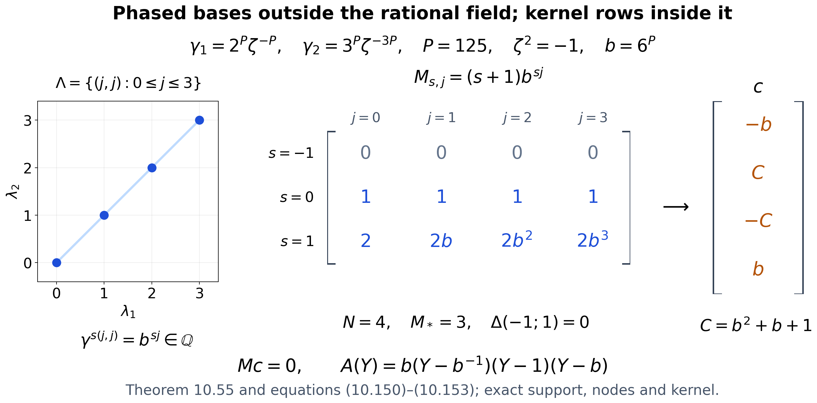
Figure 10.9. In \(\mathbb Q_5\), choose the root \(\zeta^2=-1\) with \(\zeta\equiv2\pmod5\), and put \(P=125\), \(G_0=2\), \(\alpha_0=-1\), \(\theta=(2,3)\), \(d=(-P,-3P)\). Both \(\gamma_1=2^P\zeta^{-P}\) and \(\gamma_2=3^P\zeta^{-3P}\) are outside \(\mathbb Q\), but \(\gamma_1\gamma_2=6^P=b\in\mathbb Q\). For support \(\Lambda=\{(j,j):0\le j\le3\}\), reference \((0,0)\), \(k=L=1\), \(S=1\), \(T=0\), the normalized torus column is \(b^{sj}\). The drawn matrix includes the additive factor \(\Delta(s;1)=s+1\), so its first row is zero. With \(C=b^2+b+1\), its integer vector \((-b,C,-C,b)\) is a kernel vector. Equations (10.150)–(10.153) prove the general field and height mechanism; Solution 28 checks this exact example and its extra zero. The plotted support points and matrix entries are exact. Human-source context: the field reduction and initial kernel in Lemma 4.2 of Yu's free 2013 paper, cited below. Figure program.
22. The field and budget at the first fractional nodes
At a fractional node the value need not be in \(K\), even if its chosen completion is still \(K_{\mathfrak p}\). We now determine the smaller field generated by the support, and then prove the arithmetic comparison needed before the next coset extraction.
The support-generated root field
Theorem 10.56 (the field of the normalized fractional monomials). Retain the saturated Kummer and phase data of Section 20: in particular \(\mu_q\subset K\), \(q\ne p\), \(q\nmid P\), and \([K(\beta,\rho_1,\ldots,\rho_r):K]=q^{r+1}\), with \(\beta^q=\alpha_0\), \(\rho_i^q=\theta_i\). Suppose \(\gamma_i\in K_{\mathfrak p}\) have \(v_p(\gamma_i-1)>1/(p-1)\), and use the compatible principal roots \(\eta_i=\exp(q^{-1}\log\gamma_i)=\rho_i^P\xi^{d_i}\) of Corollary 10.52.
Let \(\Lambda\) be a nonempty finite support with \(\boldsymbol d\cdot\lambda\equiv\varepsilon\pmod{G_0}\), and fix \(\lambda_0\in\Lambda\). Define
\[ \begin{aligned} m_\lambda&=\lambda-\lambda_0,& w_\lambda&=\frac{\boldsymbol d\cdot m_\lambda}{G_0}\in\mathbb Z,\\ g&=\gcd(G_0,d_1,\ldots,d_r),& G_*&=G_0/g,\qquad d_{*i}=d_i/g,\\ v_\lambda&=(w_\lambda,Pm_{\lambda1},\ldots,Pm_{\lambda r}) \in\mathbb F_q^{r+1},& h_\Lambda&=\dim_{\mathbb F_q}\langle v_\lambda:\lambda\in\Lambda\rangle,\\ U_\lambda&=\eta^{m_\lambda},& E_\Lambda&=K(U_\lambda:\lambda\in\Lambda). \end{aligned} \tag{10.154} \]Then
\[ P G_*(v_\lambda)_0-\sum_i d_{*i}(v_\lambda)_i=0,\qquad h_\Lambda\le r,\qquad [E_\Lambda:K]=q^{h_\Lambda},\qquad (E_\Lambda)_{\mathfrak P}=K_{\mathfrak p} \tag{10.155} \]for the prime \(\mathfrak P\) selected by these principal roots. The first relation is a nonzero linear equation over \(\mathbb F_q\). In particular the global degree can increase while the chosen local degree stays one.
Proof. Cancelling the positive gcd gives \(G_*w_\lambda=\sum_i d_{*i}m_{\lambda i}\), and \(\gcd(G_*,d_{*1},\ldots,d_{*r})=1\). Multiply by \(P\) and reduce modulo \(q\) to obtain the relation in (10.155). If \(q\nmid G_*\), its first coefficient is nonzero, since \(q\nmid P\). If \(q\mid G_*\), at least one \(d_{*i}\) is nonzero modulo \(q\). Thus it defines a hyperplane of dimension \(r\), proving \(h_\Lambda\le r\). Cancelling the gcd is essential: the unreduced equation can otherwise be the identity \(0=0\).
The phase congruence and the compatible roots give \[ U_\lambda=\beta^{w_\lambda}\prod_i\rho_i^{Pm_{\lambda i}}, \qquad U_\lambda^q=\alpha_0^{w_\lambda}\prod_i\theta_i^{Pm_{\lambda i}}\in K. \] Choose \(\lambda_1,\ldots,\lambda_h\), \(h=h_\Lambda\), whose residue vectors form a basis of the support span. Express any \(v_\lambda\) as \(\sum_j a_jv_{\lambda_j}\), with \(0\le a_j<q\). The corresponding integer exponent vectors differ by \(q(z_0,z_1,\ldots,z_r)\). The displayed exact monomial identity therefore gives \[ U_\lambda=\alpha_0^{z_0}\prod_i\theta_i^{z_i} \prod_{j=1}^h U_{\lambda_j}^{a_j}. \] Consequently the \(h\) selected roots generate \(E_\Lambda\), and their q-th powers lie in \(K\), so its degree is at most \(q^h\).
For the reverse bound, the monomials \(\prod_jU_{\lambda_j}^{a_j}\), \(0\le a_j<q\), have distinct residue vectors \(\sum_j a_jv_{\lambda_j}\). Reduce their exponents in the full root field \(K(\beta,\rho_1,\ldots,\rho_r)\). Its degree is \(q^{r+1}\), so the root monomials with exponents in \(\{0,\ldots,q-1\}^{r+1}\) are a basis by Theorem 10.47. Our \(q^h\) monomials are nonzero \(K\)-multiples of distinct elements of that basis, and are therefore independent. This proves the exact degree, including \(h=0\).
Each \(\eta_i\) lies in \(K_{\mathfrak p}\) by the exponential proof in Lesson 9, hence \(E_\Lambda\subset K_{\mathfrak p}\). Its closure contains the closure \(K_{\mathfrak p}\) of \(K\), and is contained in \(K_{\mathfrak p}\). Thus its chosen completion is precisely \(K_{\mathfrak p}\). The absolute ramification index and residue degree at \(\mathfrak P\) are the original \(e,f\). \(\square\)
A nonzero fractional prepared value
Corollary 10.57 (the phase-sensitive fractional arithmetic budget). Take the support of Theorem 10.56, integers \(I\ge0,k,L\ge1\), a nonzero coefficient vector \(c\in K^N\), \(N=kL|\Lambda|\), and integer Euler arguments \(C_j(m_\lambda)\). Put \(D=kL\), \(A_i=\max_\lambda|m_{\lambda i}|\), \(\delta=\min_jv_p(c_j)\), and take \(x=s/q\), \(s\in\mathbb Z\), with \(|x|\le X\). Let \(V=\Psi_I(s/q;\boldsymbol t)\) be the prepared value whose torus term is \(U_\lambda^s\) and whose additive argument is \(q^{-I}x+a\). If \(t_0>D\), it is zero. Otherwise it belongs to \(E_\Lambda\), and if it is nonzero,
\[ \begin{aligned} v_p(V)-\delta\le \mathcal A_{\mathrm{frac},\boldsymbol t}(X) :=\frac{q^{h_\Lambda}[K:\mathbb Q]}{ef\ln p}\biggl(& \min\{h_\infty(c)+\ln N,h_2(c)+\tfrac12\ln N\}\\ &+\ln\mathcal H_I(X;\boldsymbol t) +\Xi_{I,1,t_0}\ln q +2PX\sum_iA_i h(\theta_i)\biggr). \end{aligned} \tag{10.156} \]Here \(\mathcal H_I\) and \(\Xi_{I,1,t_0}\) are the already proved scalar majorant and q-clearing exponent of (10.123) and (10.115).
Proof. Every torus term lies in \(E_\Lambda\), and every prepared scalar is rational, so \(V\in E_\Lambda\). Lemma 10.28 and Theorem 10.41 clear each scalar's denominator by \(q^{\Xi_{I,1,t_0}}\), with no denominator at any other prime; Theorem 10.44 bounds its ordinary absolute value by \(\mathcal H_I(X;\boldsymbol t)\).
At every place of \(E_\Lambda\), taking the absolute value of \(U_\lambda^q\) removes the root-of-unity phase. Its signed torus contribution is bounded by \[ \sum_i \frac{P|s|A_i}{q} \ln\max\{|\theta_i|_v,|\theta_i|_v^{-1}\}. \] The torus terms are units at \(\mathfrak P\). Summing this contribution outside that prime is therefore at most \(2[E_\Lambda:\mathbb Q]PX\sum_iA_i h(\theta_i)\), by the same inverse-height identity as in Theorem 10.41. The coefficient heights retain their values over \(K\): each archimedean embedding is repeated \([E_\Lambda:K]\) times, and the local degrees over a finite place sum to that same factor.
Now repeat the full coefficient-normalized product-formula argument of Theorem 10.41 over \(E_\Lambda\), retaining its Euclidean and maximum coefficient bounds and the new scalar majorant. Theorem 10.56 gives \([E_\Lambda:\mathbb Q]=q^{h_\Lambda}[K:\mathbb Q]\) and the unchanged \(e,f\) at the selected prime. These are exactly the factor and all terms in (10.156). \(\square\)
The unchanged completion does not remove \(q^{h_\Lambda}\). Nor does a high valuation at the principal-root prime give that valuation at the other primes of the global field.
Closing the first fractional-node extension
Corollary 10.58 (a proved first fractional extension). Retain the phase family of Corollary 10.57 and all selected-basis, slope, normality and projection hypotheses of Corollary 10.40 for its local curve \(\gamma^x=\exp(x\log\gamma)\). Suppose its prepared values vanish at all integers \(|s|\le R\) through total order \(T\), where \(R\ge1,T\ge0\) are integers. Choose an integer \(\mu\ge1\) with \(T'=T-\mu+1\ge0\), and put \(n=2R+1\), \(B=\lfloor\log_p(2R)\rfloor\), \(C_0=\max\{v_p(v(k)),v_p(b_n)\}\), \(M_0=\max\{B,C_0\}\). Let \(\mathcal A_{\mathrm{frac}}(X,T')= \max_{|\boldsymbol t|\le T',\,t_0\le D} \mathcal A_{\mathrm{frac},\boldsymbol t}(X)\), using (10.156). If
\[ \begin{aligned} U+D\theta+Lv_p(k!)&\ge n\mu\theta+\mu M_0,\\ (n\mu-D)\theta-Lv_p(k!)&> \mathcal A_{\mathrm{frac}}(X,T'), \end{aligned} \tag{10.157} \]then every first fractional prepared value \(\Psi_I(s/q;\boldsymbol t)\) is zero for integers \(|s|\le qX\) and \(|\boldsymbol t|\le T'\). With the larger normalizing scale, an alternative sufficient pair is
\[ \begin{aligned} U+D\left(\theta+\frac1{p-1}\right)&\ge n\mu\theta+\mu M_0,\\ (n\mu-D)\theta-\frac D{p-1}&> \mathcal A_{\mathrm{frac}}(X,T'). \end{aligned} \tag{10.158} \]Proof. The full integer input interval has separation cost \(\kappa=0\), as proved in Corollary 10.35. The first inequality of (10.157) is consequently the sufficient analytic budget (10.113). Its complete proof, retaining the loss from the selected integer Euler basis, gives \[ v_p(\Psi_I(x;\boldsymbol t))-\delta \ge(n\mu-D)\theta-Lv_p(k!) \] for every \(x\in\mathbb Z_p\) and each output index. The local curve satisfies the same proof when its separate torus bases lie outside \(K\), since that argument uses their local logarithms, prepared scalars and projection data.
For \(x=s/q\), the assumption \(q\ne p\) gives \(x\in\mathbb Z_p\). Proposition 9.4 identifies the local exponential torus factors with the principal roots \(\eta^s\), so this analytic value is exactly the algebraic value of Corollary 10.57. If it were nonzero, (10.156) would give the opposite upper bound \(\mathcal A_{\mathrm{frac}}(X,T')\), contradicting the strict second inequality. Indices with \(t_0>D\) are already zero. This proves every asserted fractional zero. Repeating the same comparison with the proved larger-scale conclusion (10.114) gives (10.158). \(\square\)
These hypotheses separate the two tasks in a numerical descent: constructing the integer input zeros and verifying the precision and strict height comparisons. Once the fractional zeros are available at nodes prime to \(q\), Theorem 10.51 performs the exact phase and support passage.
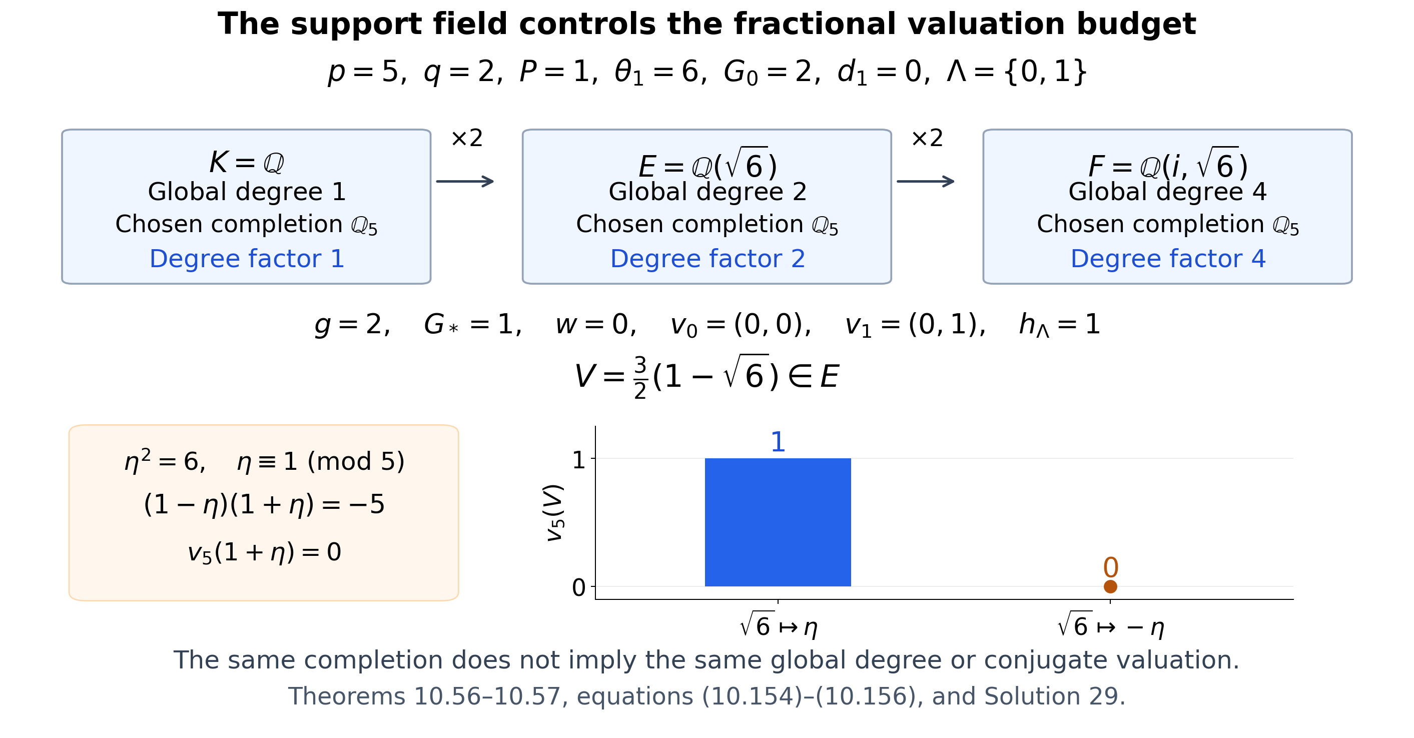
Figure 10.10. The exact example has \(K=\mathbb Q,p=5,q=2,\alpha_0=-1,\theta_1=6,P=1,G_0=2,d_1=0,\Lambda=\{0,1\}\). The cancelled relation is \(w=0\), and the support vectors span \((0,1)\) over \(\mathbb F_2\), so \(h_\Lambda=1\). The support field \(E=\mathbb Q(\sqrt6)\) has degree two; the full root field \(F=\mathbb Q(i,\sqrt6)\) has degree four. Choose the completion sending \(\sqrt6\) to \(\eta\equiv1\pmod5\). Both these roots and \(i\equiv2\pmod5\) lie in \(\mathbb Q_5\), so all three chosen completions in the diagram are \(\mathbb Q_5\). Their global-to-local degree factors are \(1,2,4\). The value \(V=\tfrac32(1-\sqrt6)\) has valuation one at this root and zero at the other root \(-\eta\); the two bars display these exact valuations. Theorem 10.56 and (10.154)–(10.155) prove the field mechanism, Corollary 10.57 proves its arithmetic budget, and Solution 29 verifies every number in this example. Human-source context: the first fractional step and product-formula field discussion in Yu's free 2013 paper, printed pp. 352 and 365–366, cited below. Figure program.
23. Heights of the actual exponent support
The torus contribution can be measured before enclosing the exponents in a coordinate box. This keeps the geometry of a support through a change of multiplicative bases and through division by \(q\). Positive and negative nodes require separate heights unless the support is symmetric.
A projective height from a support function
Let \(K\) have degree \(d\), and use the absolute values and place multiplicities of Section 14. Thus \(\sum_v\ln|z|_v=0\) for \(z\in K^\times\); a complex place is counted with multiplicity two. Take \(\theta=(\theta_1,\ldots,\theta_r)\in(K^\times)^r\), and put \(\ell_v=(\ln|\theta_1|_v,\ldots,\ln|\theta_r|_v)\). Only finitely many finite-place vectors \(\ell_v\) are nonzero. For a nonempty compact set \(C\subset\mathbb R^r\), and a nonempty finite set \(M\subset\mathbb Z^r\), define
\[ \begin{aligned} \mathfrak H_\theta(C)&=\frac1d\sum_v\sup_{u\in C}u\cdot\ell_v,\\ \mathfrak H_\theta(M)&=\mathfrak H_\theta(\operatorname{conv}M) =h_\infty((\theta^m)_{m\in M}). \end{aligned} \tag{10.159} \]The finite-set equality, and all the properties needed below, are proved next.
Theorem 10.59 (the support height). The quantities in (10.159) are finite and nonnegative. For a real vector \(a\), a real \(t\ge0\), and an integer \(s\),
\[ \begin{aligned} \mathfrak H_\theta(C+a)&=\mathfrak H_\theta(C),& \mathfrak H_\theta(tC)&=t\mathfrak H_\theta(C),\\ C\subset C'&\Longrightarrow\mathfrak H_\theta(C)\le\mathfrak H_\theta(C'),& h_\infty((\theta^{sm})_{m\in M}) &=\begin{cases} s\mathfrak H_\theta(M),&s\ge0,\\ |s|\mathfrak H_\theta(-M),&s<0. \end{cases} \end{aligned} \tag{10.160} \]If \(|m_i|\le A_i\) for every \(m\in M\), then
\[ \mathfrak H_\theta(M),\ \mathfrak H_\theta(-M) \le2\sum_i A_i h(\theta_i). \tag{10.161} \]These heights are unchanged by extending \(K\). Root-of-unity factors attached separately to the monomial coordinates change neither height.
Proof. The support function of a finite convex hull is the maximum over its original points: a convex combination cannot exceed their maximum, and those points belong to the hull. Since \(\ln|\theta^m|_v=m\cdot\ell_v\), its normalized sum is exactly the maximum projective height in (10.159). All sums are finite. For a compact \(C\), translating by \(a\) adds \(a\cdot\ell_v\) at each place. The product formula for each \(\theta_i\) makes the sum of these additions zero. Translating by the negative of any point of \(C\) places zero in the set; every resulting support function is then nonnegative. This proves nonnegativity.
Nonnegative scaling multiplies each support function by \(t\), including \(t=0\); inclusion increases it. Taking \(s\ge0\) in the monomial identity multiplies the local maximum by \(s\), while \(s<0\) replaces \(M\) by \(-M\). This proves (10.160). At any place, the box bounds both support functions by \(\sum_i A_i|\ln|\theta_i|_v|\). The sum of the positive logarithms for one element is \(d h(\theta_i)\), and the product formula says the sum of the negative logarithms has the same absolute value. Their total is \(2d h(\theta_i)\), proving (10.161).
For completeness, an extension \(E/K\) repeats each archimedean embedding \([E:K]\) times. At a finite place \(v\), the logarithm of the norm absolute value at a place \(w\) of \(E\) restricting to \(v\) is multiplied by \([E_w:K_v]\). The local degrees sum to \([E:K]\), by the places identities proved in Absolute values and places. The support function is homogeneous for these positive multipliers. Thus its unnormalized place sum is multiplied by \([E:K]\); dividing by \([E:\mathbb Q]=[E:K]d\) preserves its value. Every root of unity has absolute value one at every place, by its finite-order equation, so its coordinate factors make no contribution. \(\square\)
Symmetry is a sufficient reason for the two signs to agree; it is not automatic. Over \(\mathbb Q\), for \(\theta=(2,3)\) and \(M=\{(0,0),(1,0),(0,1)\}\), the monomial vector is \((1,2,3)\), of height \(\ln3\). The inverse vector \((1,1/2,1/3)\) becomes the primitive integer vector \((6,3,2)\), of height \(\ln6\). These are \(\mathfrak H_\theta(M)\) and \(\mathfrak H_\theta(-M)\).
Contraction and the original multiplicative bases
Theorem 10.60 (a height envelope for the divided support). Let \(C\subset\mathbb R^r\) be nonempty and compact. If a finite nonempty support \(M_I\) satisfies \(M_I\subset q^{-I}C-x_I\), then
\[ \mathfrak H_\theta(M_I)\le q^{-I}\mathfrak H_\theta(C),\qquad \mathfrak H_\theta(-M_I)\le q^{-I}\mathfrak H_\theta(-C). \tag{10.162} \]The support passage \(M_{I+1}=\{(m-m_*)/q:m\text{ in a retained coset of }M_I\}\) retains this form of containment. A further restriction of the support and any choice of reference point retain the bound.
Suppose also that \(\alpha_1,\ldots,\alpha_n\in K^\times\), that \(B=(b_{ji})\) is a real \(n\)-by-\(r\) matrix of rank \(r\), and that a positive integer \(\tau\) satisfies \(\tau b_{ji}\in\mathbb Z\) and \(\theta_i^\tau=\prod_j\alpha_j^{\tau b_{ji}}\). For finite \(D_j\ge0\), put \(C_B=\{u: |(Bu)_j|\le D_j,\ 1\le j\le n\}\). Then \(C_B\) is compact and centrally symmetric, and
\[ \mathfrak H_\theta(C_B)=\mathfrak H_\theta(-C_B) \le2\sum_{j=1}^nD_j h(\alpha_j),\qquad \mathfrak H_\theta(\pm M_I) \le2q^{-I}\sum_jD_jh(\alpha_j) \quad(M_I\subset q^{-I}C_B-x_I). \tag{10.163} \]Proof. Translation, scaling and inclusion in Theorem 10.59 give (10.162). The next retained support is contained in \(q^{-(I+1)}C-(x_I+m_*)/q\), so induction preserves exactly this envelope. Restriction uses inclusion; changing reference uses translation.
Choose an invertible \(r\)-by-\(r\) row minor of \(B\). Its inverse bounds each coordinate of \(u\in C_B\) by a fixed finite linear combination of the \(D_j\). Thus \(C_B\) is bounded; its defining inequalities make it closed. To see directly that its support maximum is attained, take a sequence approaching the supremum of a linear function. Successive bisection of a bounded coordinate interval chooses an infinite subsequence in nested closed intervals of lengths tending to zero. Repeating this for the finitely many coordinates gives a convergent subsequence. Its limit lies in the closed set, and the finite linear sum tends to its value there. This also proves the required compactness in finite dimension.
Taking absolute values of the \(\tau\)-power identities and cancelling \(\tau\) gives \(\ell_v=B^{\mathsf T}(\ln|\alpha_j|_v)_j\). Consequently \[ u\cdot\ell_v=\sum_j(Bu)_j\ln|\alpha_j|_v \le\sum_jD_j|\ln|\alpha_j|_v| \qquad(u\in C_B). \] Sum this inequality and use the inverse-height identity proved in Theorem 10.59. The set \(C_B\) is centrally symmetric because its inequalities use absolute values. Combining the resulting bound with (10.162) proves (10.163). \(\square\)
The same height bound holds for a nonempty affine box constraint \(|(Bu)_j-z_j|\le D_j\), with arbitrary real \(z_j\). Indeed its local support maximum is at most \(\sum_j z_j\ln|\alpha_j|_v+\sum_jD_j|\ln|\alpha_j|_v|\). The first sum disappears after summing over places, by the product formula, even if \(z\) is outside the image of \(B\). Thus the bound uses the half-widths in the original coordinates and follows the original torus products through a change of basis. An enclosing box in the new coordinates is unnecessary.
The coefficient and nonzero-value budgets
Corollary 10.61 (initial coefficients with the support height). Retain every hypothesis and notation of Theorem 10.55, including \(N>M_*\), and put \(M=\Lambda-\lambda_0\), \(H_+=\mathfrak H_\theta(M)\), \(H_-=\mathfrak H_\theta(-M)\). Define \(b(s)=PsH_+\) for \(s\ge0\), and \(b(s)=P|s|H_-\) for \(s<0\). Its nonzero integral kernel exists with
\[ \begin{aligned} h_\infty(c)\le h_2(c)\le& \tfrac12\ln N+\frac{\ln|\Delta_K|}{2d}\\ &+\frac1{N-M_*}\sum_{s=-S}^S\sum_{\boldsymbol t\in\mathcal J_T} \left(\tfrac12\ln N+\ln\mathcal H_0(|s|;\boldsymbol t)+b(s)\right), \end{aligned} \tag{10.164} \]and hence with
\[ \begin{aligned} h_2(c)\le&\ \tfrac12\ln N+\frac{\ln|\Delta_K|}{2d}\\ &+\frac{M_*}{N-M_*}\left( \tfrac12\ln N+\ln\mathcal B_0^*(S,T) +\frac{PS(S+1)}{2(2S+1)}(H_++H_-)\right). \end{aligned} \tag{10.165} \]Both bounds are at least as strong as their respective bounds (10.152) and (10.153).
Proof. The normalized torus monomials in a row are \(\alpha_0^{s w_\lambda}\theta^{Ps m_\lambda}\). At an archimedean embedding, their maximum times \(\sqrt N\mathcal H_0(|s|;\boldsymbol t)\) bounds the row's Euclidean norm. At a finite place their maximum bounds its maximum norm, since every scalar is an integer. The phase has absolute value one. Summing the logarithms of these maxima gives exactly \(b(s)\), by Theorem 10.59. The support contains zero, so each local torus maximum is at least one; the scalar majorant is also at least one, by Theorem 10.44. These are valid row factors in the completely proved weighted Siegel lemma (8.40), with a zero row allowed factor one. Its proof therefore gives (10.164) over \(K\), exactly as in Theorem 10.55. The same row system, integral vector and polynomial-independence argument impose every original zero.
The positive and negative node sums are both \(S(S+1)/2\). There are \(J_T\) rows at each node and \(M_*=(2S+1)J_T\). Using the uniform scalar bound gives (10.165). Finally (10.161) bounds each of \(H_+,H_-\) by \(2\sum_iA_i h(\theta_i)\); substitution gives the original two torus terms, without changing any other term. \(\square\)
Corollary 10.62 (the support budget for a nonzero value). In the phase family of Theorem 10.55, suppose the \(\gamma_i\) are units at the chosen prime, and consider an integer-node prepared value \(V=\Psi_I(s;\boldsymbol t)\), with \(t_0\le D\). Put \(C_c=\min\{h_\infty(c)+\ln N,h_2(c)+\tfrac12\ln N\}\) and \(\delta=\min_jv_p(c_j)\). If \(V\ne0\), then
\[ v_p(V)-\delta\le\frac d{ef\ln p} \left(C_c+\ln\mathcal H_I(|s|;\boldsymbol t) +\Xi_{I,0,t_0}\ln q+b(s)\right). \tag{10.166} \]In the first fractional family of Corollary 10.57, with its support field \(E_\Lambda\), the nonzero value at \(x=s/q\) satisfies instead
\[ v_p(V)-\delta\le\frac{q^{h_\Lambda}d}{ef\ln p} \left(C_c+\ln\mathcal H_I(|s|/q;\boldsymbol t) +\Xi_{I,1,t_0}\ln q+\frac{b(s)}q\right). \tag{10.167} \]Uniformly for \(|s|\le X\) in the integer case and \(|s|\le qX\) in the fractional case, the torus term may be replaced by
\[ PX\max\{H_+,H_-\}. \tag{10.168} \]The corresponding strict zero-forcing comparisons of Theorem 10.43 and Corollaries 10.54 and 10.58 remain valid with these smaller budgets, under all their original analytic and field hypotheses.
Proof. For the integer case the phase congruence puts every torus monomial in \(K\). Repeat Theorem 10.41's product formula after dividing by a coefficient of minimum local valuation. Its coefficient contribution is \(C_c\); Theorem 10.44 supplies the individual scalar bound, and (10.115) supplies its clearing exponent. At each place the torus contribution is the maximum of the logarithms of \(\theta^{Ps m_\lambda}\), with the phase removed. Its sum is \(d b(s)\). Its omitted contribution at the chosen prime is zero: the \(\gamma_i\) are units, and taking absolute values of \(\gamma_i=\theta_i^P\zeta^{d_i}\) shows that the \(\theta_i\) are units there. These local maxima are nonnegative because \(0\in M\). This proves (10.166).
In the fractional case, \(U_\lambda^q=\alpha_0^{w_\lambda}\theta^{Pm_\lambda}\). Taking local logarithmic absolute values divides the preceding torus maximum by \(q\), and its field-normalized sum is \(b(s)/q\), by the field-invariance proof of Theorem 10.59. Theorem 10.56 still gives the global degree \(q^{h_\Lambda}d\) and the original local \(e,f\); none of these degree factors has been discarded. The same coefficient-normalized product formula gives (10.167). The bounds on \(s\) give (10.168).
The analytic conclusions in the cited zero-forcing proofs supply their unchanged lower bounds for the same valuations. A strict inequality between that lower bound and the new arithmetic upper bound again contradicts \(V\ne0\). Taking the maximum over the asserted output indices proves all the same zeros. This changes only the torus height estimate; every slope, depth, order and field condition remains a hypothesis. \(\square\)
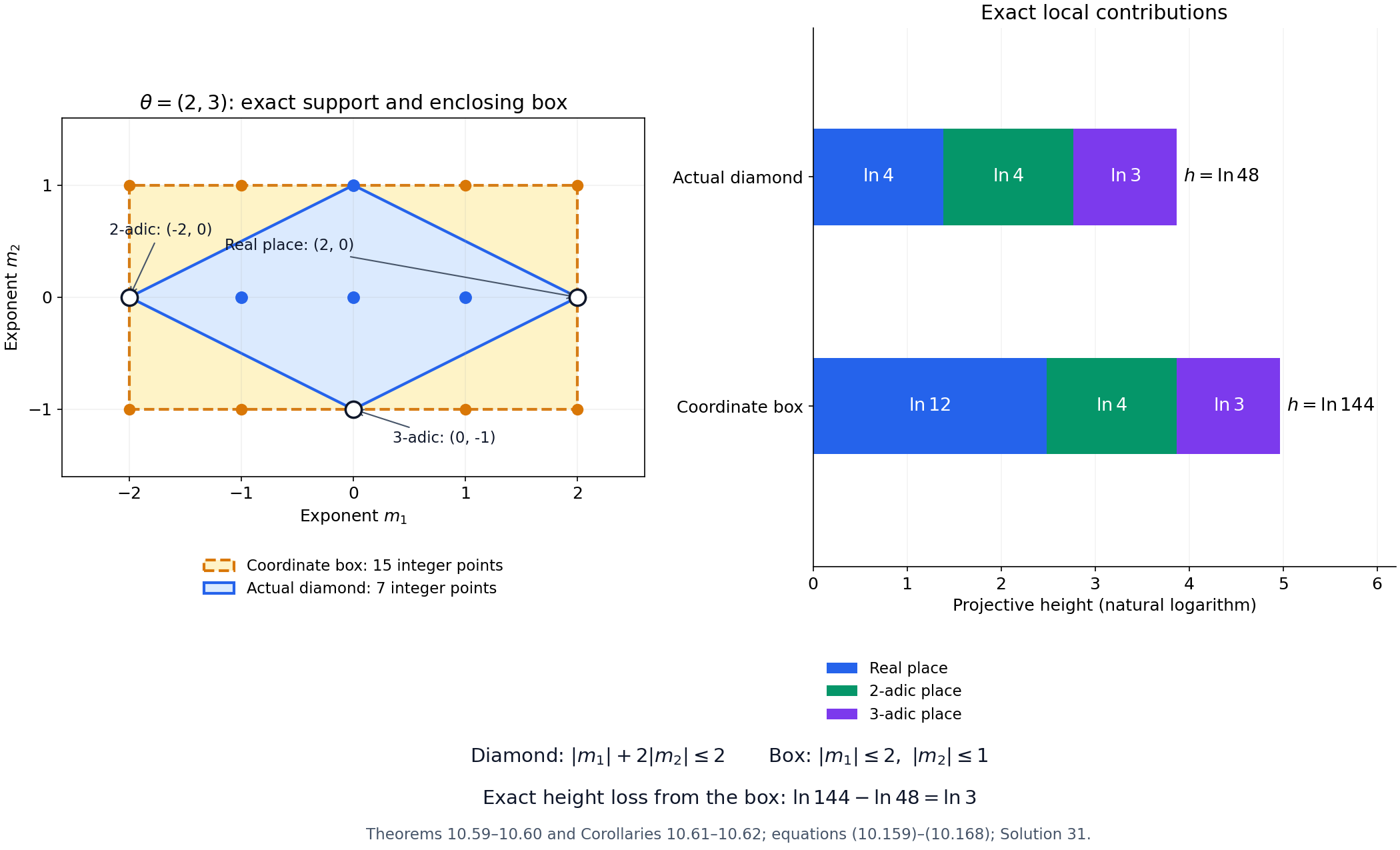
Figure 10.11. Over \(\mathbb Q\), with \(\theta=(2,3)\), the diamond \(C=\{(u_1,u_2):|u_1|+2|u_2|\le2\}\) has seven integer points; its enclosing box \([-2,2]\times[-1,1]\) has fifteen. At the real, 2-adic and 3-adic places the diamond's support contributions are \(\ln4,\ln4,\ln3\), attained respectively at \((2,0),(-2,0),(0,-1)\). The box contributions are \(\ln12,\ln4,\ln3\). Their exact projective heights are therefore \(\ln48\) and \(\ln144\). The bar lengths are numerical renderings of these labelled exact logarithms. The polygon, lattice points, active points and height identities are exact. Equations (10.159)–(10.168) prove the general support, contraction and budget mechanism; Solution 31 checks the primitive monomial vectors and a divided-support example. Human-source context: the original-coordinate torus identity and support containment (4.16), (5.1), and the product-formula steps (5.34)–(5.36), (7.13) in Yu's free 2013 paper, cited below. Figure program.
The enclosing-box estimate is valid, but this example loses exactly \(\ln3\) in its torus height. The support budget avoids that loss, and (10.163) retains bounds in the original bases after a multiplicative change of coordinates.
24. The field and the numerical scale of the initial kernel
The initial rows need not generate the entire ambient number field. We can construct their coefficients over the field they actually generate. Its discriminant is controlled by the heights of explicit normalized torus monomials, so an unrelated extension of the ambient field does not enter the coefficient budget.
The exact field of the row entries
Retain Theorem 10.55, and write \(M=\Lambda-\lambda_0\), \(H_+=\mathfrak H_\theta(M)\), \(H_-=\mathfrak H_\theta(-M)\). The normalized monomials and the field generated by all initial row entries are
\[ \begin{aligned} W_\lambda&=\alpha_0^{w_\lambda}\theta^{P(\lambda-\lambda_0)} \in K,\qquad W_{\lambda_0}=1,\\ E_0&=\begin{cases} \mathbb Q,&S=0,\\ \mathbb Q(W_\lambda:\lambda\in\Lambda),&S\ge1, \end{cases} \qquad d_0=[E_0:\mathbb Q]\le d. \end{aligned} \tag{10.169} \]Theorem 10.63 (initial coefficients over their row field). The field in (10.169) is exactly the smallest subfield of \(K\) containing every coefficient of the initial homogeneous system (10.150). If \(N>M_*\), that system has a nonzero coefficient vector \(c\in\mathcal O_{E_0}^N\subset\mathcal O_K^N\) giving the same nonzero Laurent polynomial and every originally specified zero.
For \(S\ge1\), choose normalized monomials \(z_1,\ldots,z_a\) that generate \(E_0\). Put \(F_j=\mathbb Q(z_1,\ldots,z_j)\), \(F_0=\mathbb Q\), so \(F_a=E_0\), and let \(e_j=[F_j:F_{j-1}]\). Omit steps of degree one, and define \(\Gamma=\sum_j(e_j-1)h(z_j)\). For \(S=0\), use the empty tower and \(\Gamma=0\). Then
\[ \frac{\ln|\Delta_{E_0}|}{2d_0} \le\frac12\ln d_0+\Gamma,\qquad \Gamma\le(d_0-1)P\min\{H_+,H_-\}. \tag{10.170} \]With \(b(s)\) as in Corollary 10.61, the coefficients can be chosen with
\[ \begin{aligned} h_\infty(c)\le h_2(c)\le& \frac12\ln(Nd_0)+\Gamma\\ &+\frac1{N-M_*}\sum_{s=-S}^S \sum_{\boldsymbol t\in\mathcal J_T} \left(\frac12\ln N+\ln\mathcal H_0(|s|;\boldsymbol t)+b(s)\right), \end{aligned} \tag{10.171} \]and therefore with
\[ \begin{aligned} h_2(c)\le&\ \frac12\ln(Nd_0)+\Gamma\\ &+\frac{M_*}{N-M_*} \left(\frac12\ln N+\ln\mathcal B_0^*(S,T) +\frac{PS(S+1)}{2(2S+1)}(H_++H_-)\right). \end{aligned} \tag{10.172} \]The actual discriminant term \(\ln|\Delta_{E_0}|/(2d_0)\) may instead be retained, replacing \(\frac12\ln d_0+\Gamma\) in either formula.
Proof. Every entry of the row at \(s\) is an integer prepared scalar times \(W_\lambda^s\). If \(S=0\), all entries are rational integers, so their field is \(\mathbb Q\). If \(S\ge1\), these expressions first show that every entry belongs to the monomial field in (10.169). Conversely take the row at \(s=1\) with derivative index zero. Its column with \(a=0,\ell=1\) and any \(\lambda\) is \(\Delta(1;k)W_\lambda=(k+1)W_\lambda\). Every Euler factor there is \(\Delta(\omega;0)=1\). Division by the nonzero rational integer \(k+1\) recovers \(W_\lambda\) from that row. Thus every field containing the entries contains each monomial, proving minimality.
The discriminant-and-generators proof, equation (8.33), gives the first bound in (10.170) for this explicit tower, including nonintegral monomials. Each selected \(z_j\) is a coordinate of the monomial vector containing \(1\). Its ordinary height is at most that vector's maximum projective height \(PH_+\): locally, the vector maximum bounds \(\max\{1,|z_j|_v\}\). The inverse vector also contains \(1\), so it bounds \(h(z_j^{-1})=h(z_j)\) by \(PH_-\). Consequently \(h(z_j)\le P\min\{H_+,H_-\}\). The integer degrees have product \(d_0\); induction using \((u-1)+(v-1)\le uv-1\) gives \(\sum_j(e_j-1)\le d_0-1\). This proves the second bound. The empty-tower case has \(d_0=1,\Delta_{E_0}=1\).
Apply the completely proved weighted Siegel lemma (8.40) over \(E_0\) to the actual representative rows. Their number \(M_*\), their integer scalar bounds and all their dependencies are unchanged. Their normalized torus row height is \(b(s)\), as in Corollary 10.61. This height can be computed over \(K\), because the row vector lies in \(E_0\) and projective heights are invariant under extension. The individual \(\theta_i\) need not lie in \(E_0\). The Euclidean row bound adds \(\frac12\ln N+\ln\mathcal H_0\) as before. The finite-place conditions give \(c\in\mathcal O_{E_0}^N\), and such elements are also algebraic integers in \(K\).
That lemma supplies \(\frac12\ln N+\ln|\Delta_{E_0}|/(2d_0)\), followed by the displayed row sum divided by \(N-M_*\). Substitution of (10.170) proves (10.171). Summing the positive and negative nodes separately proves (10.172), exactly as in (10.165). A nonzero coefficient vector still gives a nonzero polynomial by Lemma 10.29, and the same representative-row argument preserves all jets in (10.150). This proves every assertion. \(\square\)
Full widths in the original coordinates
The original torus widths can now be inserted before any numerical constants are rounded. Let \(\alpha_1,\ldots,\alpha_r\in K^\times\), and suppose the multiplicative change of basis in Theorem 10.60 satisfies, for a positive integer \(\tau\), \(\theta_i^\tau=\omega_i\prod_j\alpha_j^{\tau b_{ji}}\), where \(\omega_i\) is a root of unity and every \(\tau b_{ji}\) is integral. The root-of-unity factors contribute zero to every local logarithm, so the proof of (10.163) still applies. Suppose the original support coordinates \(B\Lambda\) lie in a translated box of full widths \(D_1,\ldots,D_r\), and put \(L_\alpha=\sum_j D_j h(\alpha_j)\). After choosing the reference point \(\lambda_0\), its original coordinates \(BM\) satisfy affine box constraints with half-widths \(D_j/2\). The affine-centre proof following (10.163) gives
\[ H_+,H_-\le L_\alpha,\qquad \Gamma\le(d_0-1)P L_\alpha. \tag{10.173} \]Here the box condition is imposed on \(Bm\); it does not require its centre to be in the image of \(B\).
Corollary 10.64 (an initial budget in the original heights). Under these hypotheses and \(N>M_*\), the initial coefficient vector may be chosen with
\[ \begin{aligned} h_2(c)\le&\ \frac12\ln(Nd_0)+(d_0-1)P L_\alpha\\ &+\frac{M_*}{N-M_*} \left(\frac12\ln N+\ln\mathcal B_0^*(S,T) +\frac{PS(S+1)}{2S+1}L_\alpha\right). \end{aligned} \tag{10.174} \]Replacing \(d_0\) everywhere by its upper bound \(d\) gives a valid further bound.
Proof. Substitute both parts of (10.173) into (10.172). The factor of two from \(H_++H_-\) cancels the two in its denominator. The replacement by \(d\) increases \(\ln d_0\) and \(d_0-1\), while all other terms stay unchanged and \(P L_\alpha\ge0\). \(\square\)
In particular a full width \(D_j\) is not a half-width \(D_j\). This distinction accounts for a factor of two in the torus contribution.
Substitution at the numerical scale
Corollary 10.65 (the scaled coefficient inequality). Suppose \(S\ge1\), \(N\ge c_*M_*\) with \(c_*>1\), and that positive numbers \(\mathcal D,c_1,c_2,\sigma_1,\ldots,\sigma_r\) satisfy
\[ h(\alpha_j)\le\sigma_j,\qquad D_j=\frac{\mathcal D}{c_1c_2rPd\sigma_j},\qquad Z=\frac{S\mathcal D}{d}. \tag{10.175} \]Then a coefficient vector with every zero in Theorem 10.63 exists with
\[ \begin{aligned} \frac{h_2(c)}Z\le& \frac{d\ln(Nd_0)}{2S\mathcal D} +\frac{d_0-1}{c_1c_2S}\\ &+\frac1{c_*-1}\left( \frac{d(\frac12\ln N+\ln\mathcal B_0^*(S,T))}{S\mathcal D} +\frac1{2c_1c_2}\left(1+\frac1{2S+1}\right)\right). \end{aligned} \tag{10.176} \]An explicit generator tower may improve the second term to \(\Gamma/Z\). If \(S\ge g>0\), the last factor \(1+1/(2S+1)\) is at most \(1+1/(2g+1)\).
Proof. Formula (10.175) gives \[ P L_\alpha=P\sum_jD_jh(\alpha_j) \le P\sum_jD_j\sigma_j =\frac{\mathcal D}{c_1c_2d}. \] Also \(M_*/(N-M_*)\le1/(c_*-1)\): divide \(N\ge c_*M_*\) by \(M_*>0\) and subtract one. Every term in the parentheses of (10.174) is nonnegative. Divide that bound by \(Z\), insert these inequalities, and use the exact identity \[ \frac{S+1}{2S+1}=\frac12\left(1+\frac1{2S+1}\right). \] This proves (10.176), including its coefficient \(\frac1{2c_1c_2}\). Retaining \(\Gamma\) in (10.172) proves the tower refinement. Finally \(S\ge g\) increases the positive denominator \(2S+1\), giving the asserted upper bound. \(\square\)
Equation (10.176) supplies a direct numerical comparison once the column surplus, scalar majorant and coefficient-field tower have been determined. It retains the full-width torus term without an ambient-field discriminant. The later zero-forcing inequalities still require their own strict comparisons.
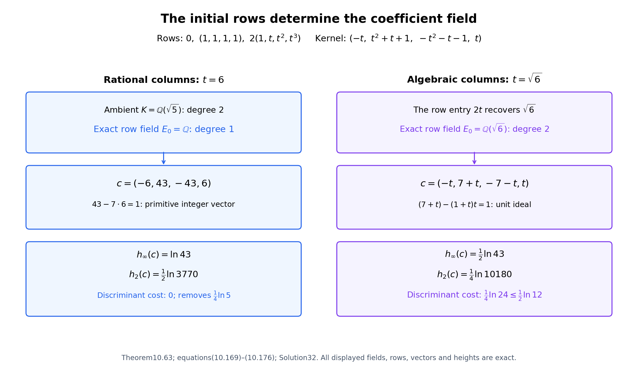
Figure 10.12. For \(k=L=S=1,T=0,\Lambda=\{0,1,2,3\},P=1\), the initial rows are \(0\), \((1,1,1,1)\), \(2(1,t,t^2,t^3)\). The vector \((-t,t^2+t+1,-t^2-t-1,t)\) is their exact integral kernel. Left: \(t=6\), with ambient \(K=\mathbb Q(\sqrt5)\), gives row field \(\mathbb Q\), vector \((-6,43,-43,6)\), and no discriminant cost. The ambient-field cost would be \(\frac14\ln5\). Right: \(t=\sqrt6\) generates row field \(\mathbb Q(\sqrt6)\), with discriminant \(24\). Its cost \(\frac14\ln24\) is retained; the generator proof bounds it by \(\frac12\ln12\). The exact coefficient heights are \(\ln43,\frac12\ln3770\) on the left and \(\frac12\ln43,\frac14\ln10180\) on the right. Theorem 10.63 and equations (10.169)–(10.176) prove the field and budget mechanism; Solution 32 verifies the rows, discriminants and heights. Human-source context: the initial coefficient-field reduction in Lemma 4.2 of Yu's free 2013 paper; the complete discriminant and Siegel inputs are proved in the earlier lesson linked above, from Matveev's free paper. Figure program.
25. Constructing enough columns in one phase class
The coefficient inequalities require a surplus of columns over equations. We now produce that surplus from the volume of a closed box, the covolume of the saturated exponent lattice and the number of possible phase classes. The boundary of the box matters when its normalized volume is an integer.
Points in a translated closed box
Theorem 10.66 (the closed-box lattice count). Let \(\mathcal L=B\mathbb Z^r\), with \(B\) an invertible real matrix, and let \(C=\prod_{j=1}^r[0,D_j]\), with every \(D_j>0\). Write
\[ \Delta=|\det B|,\qquad V=\prod_jD_j,\qquad m=\lfloor V/\Delta\rfloor. \tag{10.177} \]There are \(m+1\) distinct points \(y_0,\ldots,y_m\) of \(C\) such that all \(y_j-y_0\) lie in \(\mathcal L\). Consequently a translate of \(C\) contains \(m+1\) distinct lattice points, including zero.
If \(\mathcal L\supset\mathbb Z^r\) has finite index \(J=|\mathcal L/\mathbb Z^r|\), then
\[ \Delta=J^{-1},\qquad m=\lfloor JV\rfloor. \tag{10.178} \]Proof. Take the half-open fundamental cell \(F=B[0,1)^r\). Its translates by \(\mathcal L\) partition \(\mathbb R^r\), and its volume is \(\Delta\). For \(x\in F\), let \(n_C(x)\) count the points of \(x+\mathcal L\) in \(C\). This is a finite sum of indicator functions: boundedness of \(C-F\) bounds the integer coordinates \(B^{-1}\ell\) of any participating lattice vector. Translating each integral and using the partition gives \[ \int_F n_C(x)\,dx =\sum_{\ell\in\mathcal L}\int_{F+\ell}\mathbf1_C(y)\,dy =V. \] The volume and translation rules used here are the same ones proved in the lattice argument of Small solutions over the coefficient field. If \(V/\Delta>m\), this integral prevents \(n_C(x)\le m\) everywhere. Some coset therefore supplies \(m+1\) points.
For the equality case \(V/\Delta=m\), enlarge \(C\) about its centre by factors \(1+1/n\). Each enlarged closed box has volume strictly greater than \(m\Delta\), so it contains \(m+1\) points \(x_n+\ell_{0n},\ldots,x_n+\ell_{mn}\), with \(x_n\in F\). All participating lattice vectors lie in one fixed bounded set, because the enlarged boxes lie in the box enlarged by two and \(F\) is bounded. There are finitely many such lattice vectors. Passing to a subsequence fixes the distinct vectors \(\ell_0,\ldots,\ell_m\); a further subsequence makes \(x_n\) converge in the closed bounded cell \(B[0,1]^r\). Coordinatewise interval bisection gives this convergent subsequence, as in the proof of Theorem 10.60. The limits \(x+\ell_j\) lie in \(C\): its closed inequalities are the limits of the enlarged inequalities. Their differences are the distinct lattice differences \(\ell_j-\ell_0\). This proves the count also at integer normalized volume.
For (10.178), since every coordinate unit vector belongs to \(\mathcal L\), the matrix \(U=B^{-1}\) is integral. Multiplication by \(B^{-1}\) identifies \(\mathcal L/\mathbb Z^r\) with \(\mathbb Z^r/U\mathbb Z^r\). Its index is \(|\det U|\). Here is an integer reduction proof of that identity. Interchanging rows or columns, changing a sign, and adding an integer multiple of another row or column preserve index and absolute determinant. The Euclidean algorithm makes the first column have a positive pivot and zeros below. If an entry in its first row is not divisible by the pivot, column division and interchange produce a smaller positive pivot; repeat. This must stop because positive integers decrease. Column subtraction then clears the first row and leaves a nonsingular block of size \(r-1\). Induction diagonalizes the matrix by these operations. The quotient for a diagonal matrix has the product of the absolute diagonal entries as its index, by independent residue representatives. This is its absolute determinant. Thus \(J=|\det U|=1/\Delta\), proving (10.178). \(\square\)
The enlargement argument uses a closed box. For the open interval \(C=(0,1)\) and lattice \(\mathbb Z\), the normalized volume is one but no translate contains two lattice points.
Retaining a single phase
Lemma 10.67 (the phase-class count). Take the \(m+1\) lattice differences in Theorem 10.66 and write them as \(B\lambda_j\), with \(\lambda_j\in\mathbb Z^r\). For integers \(G_0\ge1\) and \(d_1,\ldots,d_r\), put
\[ g=\gcd(G_0,d_1,\ldots,d_r),\qquad H=G_0/g. \tag{10.179} \]There is a set \(\Lambda\) of at least \(\lceil(m+1)/H\rceil\) of these distinct integer vectors, all satisfying the same congruence \(\boldsymbol d\cdot\lambda\equiv\varepsilon\pmod{G_0}\). Moreover \(B\Lambda\subset C-y_0\).
Proof. Each phase value is a multiple of \(g\) modulo \(G_0\), so there are at most \(H\) possible values. If every class contained fewer than \(\lceil(m+1)/H\rceil\) of the \(m+1\) points, their total would be smaller than \(m+1\). Choose a class of at least that size. The map \(B\) is injective, so no points coalesce. The containment holds because every original difference was \(y_j-y_0\). This includes the case \(d_i=0\) for every \(i\), when \(g=G_0,H=1\). \(\square\)
A certified surplus of prepared columns
Corollary 10.68 (box volume supplies the initial kernel). Suppose the multiplicative and phase hypotheses of Theorem 10.55 are available for the lattice basis \(B\) and the phase data of Lemma 10.67. For integers \(k,L\ge1,S,T\ge0\), choose the retained support \(\Lambda\) there. Its number of coefficient columns satisfies
\[ \begin{aligned} kL\left\lceil\frac{\lfloor V/\Delta\rfloor+1}{H}\right\rceil &\le N=kL|\Lambda|\le kL(\lfloor V/\Delta\rfloor+1),\\ N&>\frac{kLV}{\Delta H}. \end{aligned} \tag{10.180} \]Define the support-independent row upper bound
\[ \overline J_T=\sum_{u=0}^{\min(kL,T)} \binom{T-u+r-1}{r-1},\qquad \overline M=(2S+1)\overline J_T. \tag{10.181} \]If \(kLV/(\Delta H)\ge c_*\overline M\), with \(c_*>1\), then \(N>c_*M_*\). In particular the complete integral initial kernel of Theorem 10.63 exists and its scaled budget (10.176) applies whenever its original-width hypotheses hold. The selected support retains that full-width height bound.
For a saturated lattice of index \(J\) and widths from (10.175), an explicit sufficient criterion is
\[ \frac{kLJ}{H}\, \frac{\mathcal D^r} {(c_1c_2rPd)^r\prod_j\sigma_j} \ge c_*(2S+1) \sum_{u=0}^{\min(kL,T)}\binom{T-u+r-1}{r-1}. \tag{10.182} \]Proof. The first inequality in (10.180) is the retained-class count; the upper bound follows because the retained class is a subset of the chosen \(m+1\) points. Since \(\lfloor V/\Delta\rfloor+1>V/\Delta\), and a ceiling is at least its argument, the strict inequality follows.
At additive order \(u\le\min(kL,T)\), allowing all \(r-1\) Euler directions gives \(\binom{T-u+r-1}{r-1}\) indices of order at most \(T-u\), by the divider count proved in Theorem 10.32. Every representative index in (10.126) is among these; zero Euler directions only remove duplicates. Hence \(M_*\le\overline M\). Combining this fact with (10.180) proves the strict surplus.
Pick any reference \(\lambda_0\) in the retained class. Its normalized phase differences are multiples of \(G_0\), and its original coordinates lie in \(C-y_0-B\lambda_0\). Thus all the hypotheses for the initial coefficient construction and the full-width estimate are retained. Apply Theorem 10.63 and, when (10.175) holds, Corollary 10.65. Substitution of \(\Delta=1/J\) and \(V=\mathcal D^r/[(c_1c_2rPd)^r\prod_j\sigma_j]\) gives (10.182). \(\square\)
The count certifies the initial coefficient construction. The analytic slope, derivative precision and strict nonzero-value comparisons used to extend its zeros remain separate hypotheses.
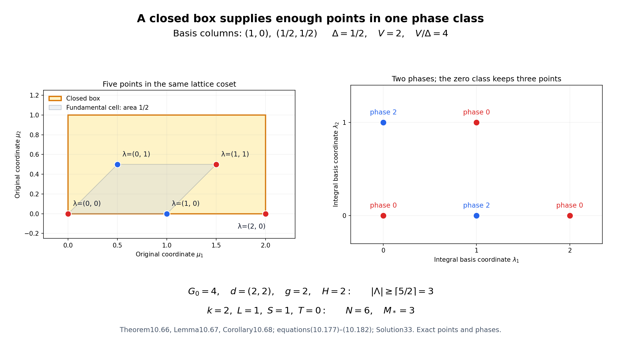
Figure 10.13. The exact lattice has basis columns \((1,0)\), \((1/2,1/2)\), covolume \(1/2\) and index two over \(\mathbb Z^2\). The closed box is \(C=[0,2]\times[0,1]\), so \(V/\Delta=4\). Five displayed points have integral basis coordinates \((0,0),(0,1),(1,0),(1,1),(2,0)\). For \(G_0=4,d=(2,2)\), there are \(H=2\) phase classes. The class \(0\) retains three points with coordinates \((0,0),(1,1),(2,0)\). At \(k=2,L=1,S=1,T=0\), they give \(N=6\) columns and \(M_*=3\) rows. The lattice, box, points and phase labels are exact. Theorem 10.66, Lemma 10.67 and Corollary 10.68 prove (10.177)–(10.182), including the integer-volume boundary case; Solution 33 verifies these data and the derivative-order limitation. Human-source context: the box and phase selection (4.18)–(4.21) in Yu's free 2013 paper, cited below. Figure program.
26. Choosing parameters with a strict coefficient surplus
The lattice count becomes useful only when it exceeds the number of prescribed jets. We give a parameter choice for which that comparison holds with all integer roundings retained. The node and jet budgets are real numbers; their floors, rather than the budgets themselves, count the equations.
The real parameters
Let \(r\ge2\), and retain the independent \(\mathfrak p\)-adic units \(\alpha_1,\ldots,\alpha_r\) in a number field of degree \(d\). Write \(e=e_{\mathfrak p}\), \(f=f_{\mathfrak p}\), and \(t=f\ln p\); thus \(ef\le d\). Let \(q=2\) for odd \(p\), and \(q=3\) for \(p=2\), with \(\zeta_3\in K\) in the latter case. Let \(q^u\) be the order of the q-primary roots of unity, and \(J=q^\nu\) the index of the q-primary saturation lattice. The roots reduce injectively: a nontrivial q-primary root in \(1+\mathfrak p\) would retain its positive finite valuation under its prime-to-\(p\) order by p-adic logarithms: power series, heights and the one-logarithm bound, Lemma 9.5, but its power is one. Their reductions form a subgroup of the finite field's group of \(p^f-1\) nonzero elements. Its distinct cosets partition that group into sets of size \(q^u\), proving \(q^u\mid p^f-1\). Use its phase coefficients from Section 20, and put
\[ \begin{aligned} G&=p^f-1,&G_0&=G/q^u,& \delta&=\gcd(G_0,d_1,\ldots,d_r),&H&=G_0/\delta,\\ \ell_d&=\max\{1,\ln d\},& \rho&=\begin{cases}58,&d\ge2,\\17,&d=1,\end{cases}& g_1&=4+\ln((r+1)d),&A&=\max\{g_1,e,t\}. \end{aligned} \tag{10.183} \]Take \(\sigma_i\ge h(\alpha_i)>0\), constants \(c_0>1\) and \(c_1,c_3,c_4>0\), and \(g_0>39\). Choose \(h\ge\max\{g_0,(r+1)t\}\). In this subsection \(h\) is this real auxiliary parameter, whereas \(h(\alpha)\) denotes Weil height. Let \(\kappa\ge0\) be the integer with \(p^{\kappa-1}(p-1)\le2e<p^\kappa(p-1)\), and set \(P=p^\kappa\). For any \(\tau\ge0\) define
\[ \begin{aligned} \vartheta&=\begin{cases}(p-2)/(p-1),&p\ge5, e=1,\\P/(2e),&\text{otherwise},\end{cases} &\theta&=\vartheta/(1+\tau),\\ c_2&=\begin{cases}7/4,&p>2,\\13/9,&p=2,\end{cases} &a_*&=\begin{cases}7/2,&p\ge5, e=1,\\26/3,&p=2,\\7,&\text{otherwise}. \end{cases} \end{aligned} \tag{10.184} \]Choose any \(\widehat\vartheta\ge\vartheta\). The explicit choices \(3/2\) at \(p=3\), \(5/4\) at \(p=5,e\ge2\), \(1\) at \(p\ge5,e=1\), \(7/6\) at \(p\ge7,e\ge2\), and \(2\) at \(p=2\) work. Indeed \(P\le2pe/(p-1)\), so \(P/(2e)\le p/(p-1)\). If \(p\ge5,e=1\), then \(\kappa=0\), \(P=1\), and \(\vartheta<1\). In particular \(c_2qP/(e\theta)\ge a_*\) in every case.
Define the positive lower budgets
\[ \begin{aligned} g_2&=\begin{cases} c_3q(r+1)^2d,&p\ge5,\ e=1,\text{ or }p\ge7,\\ c_3q(r+1)g_0e/\ln p,&p=2,3,\text{ or }p=5,\ e\ge2, \end{cases}\\ g_3&=\frac{2c_0c_1c_4}{\rho} a_*^r\frac{r^r(r+1)^r}{(r!)^2}g_1t,\\ g_4&=\frac{q(r+1)g_3}{c_1\widehat\vartheta t} \begin{cases}1,&e=1\text{ and }(p\ge5\text{ or }d=1),\\g_1^{-1},&\text{otherwise},\end{cases}\\ g_5&=\frac{c_3q(r+1)g_3}{c_1c_4g_1t}, &1+\epsilon&=\left(1+\frac{r+1}{2g_4}\right)^r. \end{aligned} \tag{10.185} \]Here the \(d=1\) alternative in \(g_4\) is compatible with \(p=3,e=1\); \(p=2,d=1\) cannot meet \(\zeta_3\in K\). Set
\[ \begin{aligned} x&=\nu\ln q,\\ \gamma&=\frac{q^\nu hA}{(h+x)(A+x)},\\ S&=\frac{c_3q(r+1)d(h+x)}t,\\ \mathcal D&=\frac{\gamma}{q^{\nu+u}} (1+\epsilon)(2+g_2^{-1})c_0c_1c_4 \left(\frac{c_2qPr(r+1)}{e\theta}\right)^r\frac1{r!}\\ &\quad{}\times \max\left\{\frac{p^f}{\delta t^r},\frac{\mathrm e^r}{r^r}t\right\} d^{r+1}\ell_d\prod_i\sigma_i\,(A+x),\\ T&=\frac{q(r+1)\mathcal D}{c_1\theta et},\\ k&=\lfloor h+x-1\rfloor+1=\lfloor h+x\rfloor,\\ \widetilde D_0&=\frac{S\mathcal D}{c_1c_4kd(A+x)},\\ L&=\lfloor\widetilde D_0\rfloor+1,\\ D_i&=\frac{\mathcal D}{c_1c_2rPd\sigma_i}. \end{aligned} \tag{10.186} \]The exponential constant \(\mathrm e=\exp(1)\) in this formula is different from the ramification index \(e\). The additive factors of the prepared family have precisely \(k\) choices of degree index and \(L\) choices of positive power, as in Lemma 10.29.
Lemma 10.69 (the saturation factor). The parameters above satisfy \(1\le\gamma\le q^\nu\).
Proof. With \(x\ge0\), \(\gamma=\exp(x)hA/((h+x)(A+x))\). The logarithmic derivative with respect to \(x\) is \(1-(h+x)^{-1}-(A+x)^{-1}>0\), because \(h>39\) and \(A\ge g_1>5\). At \(x=0\) the value is one. The upper bound follows from \((h+x)(A+x)\ge hA\). \(\square\)
Lower bounds and the rounded equation count
Lemma 10.70 (lower budgets without lost floors). We have
\[ \begin{gathered} S\ge g_2,\qquad \frac{\mathcal D}{A+x}\ge\frac{g_3}{g_1},\qquad \mathcal D\ge g_3,\qquad T\ge g_4,\\ \widetilde D_0\ge g_5,\qquad \widetilde D_0<L\le(1+g_5^{-1})\widetilde D_0,\\ \binom{\lfloor T\rfloor+r}{r} \le(1+\epsilon)\frac{T^r}{r!}. \end{gathered} \tag{10.187} \]Proof. In the first alternative for \(g_2\), use \(h+x\ge(r+1)t\) in \(S\). In the second, use \(h+x\ge g_0\) and \(d/f\ge e\). These give both stated lower bounds, including \(p=5,e\ge2\).
The q-primary lattice lies in the full saturation lattice of Theorem 10.18. Its index is \(q^\nu\), and \(w_K\ge q^u\). Consequently (10.55) gives
\[ d^{r+1}\ell_d\prod_i\sigma_i \ge \frac{q^{\nu+u}}{\rho}\frac{r^r}{r!\mathrm e^r}. \tag{10.188} \]For \(d\ge2\), replacing \(\ln d\) by the larger \(\ell_d\) preserves this bound; at \(d=1\) the degree and logarithmic factors equal one. The maximum in (10.186) is at least \((\mathrm e^r/r^r)t\). Combine this fact with (10.188), \(\gamma\ge1\), \((1+\epsilon)(2+g_2^{-1})\ge2\), and \(c_2qP/(e\theta)\ge a_*\). This yields \(\mathcal D/(A+x)\ge g_3/g_1\), including every displayed constant. Since \(A+x\ge g_1\), it also yields \(\mathcal D\ge g_3\).
If the first alternative in \(g_4\) applies, \(e=1\); use \(\mathcal D\ge g_3\) and \(\theta\le\widehat\vartheta\). Otherwise use the stronger bound \(\mathcal D\ge g_3(A+x)/g_1\) and \(A+x\ge e\). Both give \(T\ge g_4\).
We have \(0<k\le h+x\). Substitute the formula for \(S\) into \(\widetilde D_0\), and then use the stronger bound for \(\mathcal D\): \[ \widetilde D_0= \frac{c_3q(r+1)(h+x)\mathcal D}{c_1c_4kt(A+x)} \ge\frac{c_3q(r+1)g_3}{c_1c_4g_1t}=g_5. \] For any positive real \(y\), \(y<\lfloor y\rfloor+1\le y+1\). Taking \(y=\widetilde D_0\) proves both assertions about \(L\), including the strict inequality when \(y\) is an integer.
Finally, \[ \binom{\lfloor T\rfloor+r}{r} \le\frac1{r!}\prod_{j=1}^r(T+j) \le\frac1{r!}\left(T+\frac{r+1}{2}\right)^r. \] The last inequality follows from the concavity of \(\ln\): its second derivative is \(-z^{-2}<0\), so the sum of the logarithms is at most \(r\) times the logarithm of their average. Divide by \(T^r\), and use \(T\ge g_4\) and (10.185). This proves the last line of (10.187). \(\square\)
Theorem 10.71 (the parameter choice supplies a kernel). Use the closed box with widths \(D_i\) and choose its single phase class as in Lemma 10.67. In the prepared system impose every node \(|s|\le S\) with integer \(s\), and every jet of total order at most the real number \(T\). Write \(s_0=\lfloor S\rfloor\), \(t_0=\lfloor T\rfloor\), let \(N=kL|\Lambda|\), and let \(M_*\) be the actual representative row count. Put
\[ c_{01}=c_0\ell_d\frac{p^f}{p^f-1}>1. \tag{10.189} \]Then
\[ \begin{aligned} N&>\frac{kLq^\nu D_1\cdots D_r}{H} >c_{01}(2S+1)\binom{t_0+r}{r}\\ &\ge c_{01}(2s_0+1)\binom{t_0+r}{r} \ge c_{01}M_*. \end{aligned} \tag{10.190} \]In particular a nonzero global-integral coefficient vector and polynomial with all these zeros and jets exist, with the field and height conclusions of Lemma 10.63.
Proof. The first strict inequality is (10.180), with \(J=q^\nu\), \(\Delta=1/J\), and \(H=G/(q^u\delta)\). For the next comparison keep all widths in (10.186), and write \(V=\prod_iD_i\). Since \(L>\widetilde D_0\), \[ \frac{kLq^\nu V}{H}> \frac{Sq^{\nu+u}\delta\mathcal D^{r+1}} {c_1^{r+1}c_4c_2^rr^rP^rd^{r+1}(A+x)G\prod_i\sigma_i}. \] Divide by \((2S+1)(1+\epsilon)T^r/r!\). Substitute (10.186) for \(\mathcal D\). The degree factors, widths and normalization factors cancel, leaving \[ \frac{S(2+g_2^{-1})}{2S+1} \frac{\gamma c_0\ell_d\delta t^r}{G} \max\left\{\frac{p^f}{\delta t^r},\frac{\mathrm e^r}{r^r}t\right\} \ge c_{01}. \] Indeed \(S\ge g_2\) makes the first factor at least one, \(\gamma\ge1\), and the first member of the maximum gives \(p^f\). The binomial inequality (10.187) proves the second strict inequality in (10.190). A derivative order is an integer, so an order at most \(T\) is exactly an order at most \(t_0\); similarly there are exactly \(2s_0+1\) nodes. Counting all \(r\) derivative directions gives \(\binom{t_0+r}{r}\) rows per node by the divider argument of Theorem 10.32. Removing zero additive orders or duplicate Euler directions only decreases the representative count. This proves the remaining inequalities.
Since \(N>M_*\), the completely proved integral Siegel argument in Lemma 10.63 applies over the actual row field, with no unproved estimate used in place of an equation. Its nonzero vector gives a nonzero polynomial by Lemma 10.29. \(\square\)
The height term with a real node budget
Corollary 10.72 (the rounded mean torus contribution). In this kernel let \(d_0\) be the row-field degree, let \(\mathcal H_0\) be the scalar row bound from Lemma 10.63 with node budget \(s_0\) and jet budget \(t_0\), and put \(Z=S\mathcal D/d\) and \(L_\alpha=\sum_iD_i h(\alpha_i)\). Then
\[ \begin{aligned} \frac{h_2(\boldsymbol c)}Z \le{}&\frac{\tfrac12\ln(Nd_0)}Z +\frac{d_0-1}{c_1c_2S}\\ &+\frac1{c_{01}-1}\left[ \frac{\tfrac12\ln N+\ln\mathcal H_0}Z +\frac{1+1/(2g_2)}{2c_1c_2} \right]. \end{aligned} \tag{10.191} \]Proof. Apply (10.174) at the integer budget \(s_0\), and use \(N>c_{01}M_*\) from (10.190). The full original width bound and \(\sigma_i\ge h(\alpha_i)\) give \(PL_\alpha\le\mathcal D/(c_1c_2d)\), so the generator term divided by \(Z\) is at most \((d_0-1)/(c_1c_2S)\). The exact mean of the absolute integer nodes is \(s_0(s_0+1)/(2s_0+1)\). It satisfies \[ \frac{s_0(s_0+1)}{2s_0+1} =\frac{s_0}{2}+\frac14-\frac1{4(2s_0+1)} \le\frac S2+\frac14. \] Thus its contribution divided by \(Z\) is at most \((1+1/(2S))/(2c_1c_2)\le(1+1/(2g_2))/(2c_1c_2)\). Substitution proves (10.191). This leaves the scalar row and row-field generator costs explicit; each must still be included in a numerical zero-forcing comparison. \(\square\)
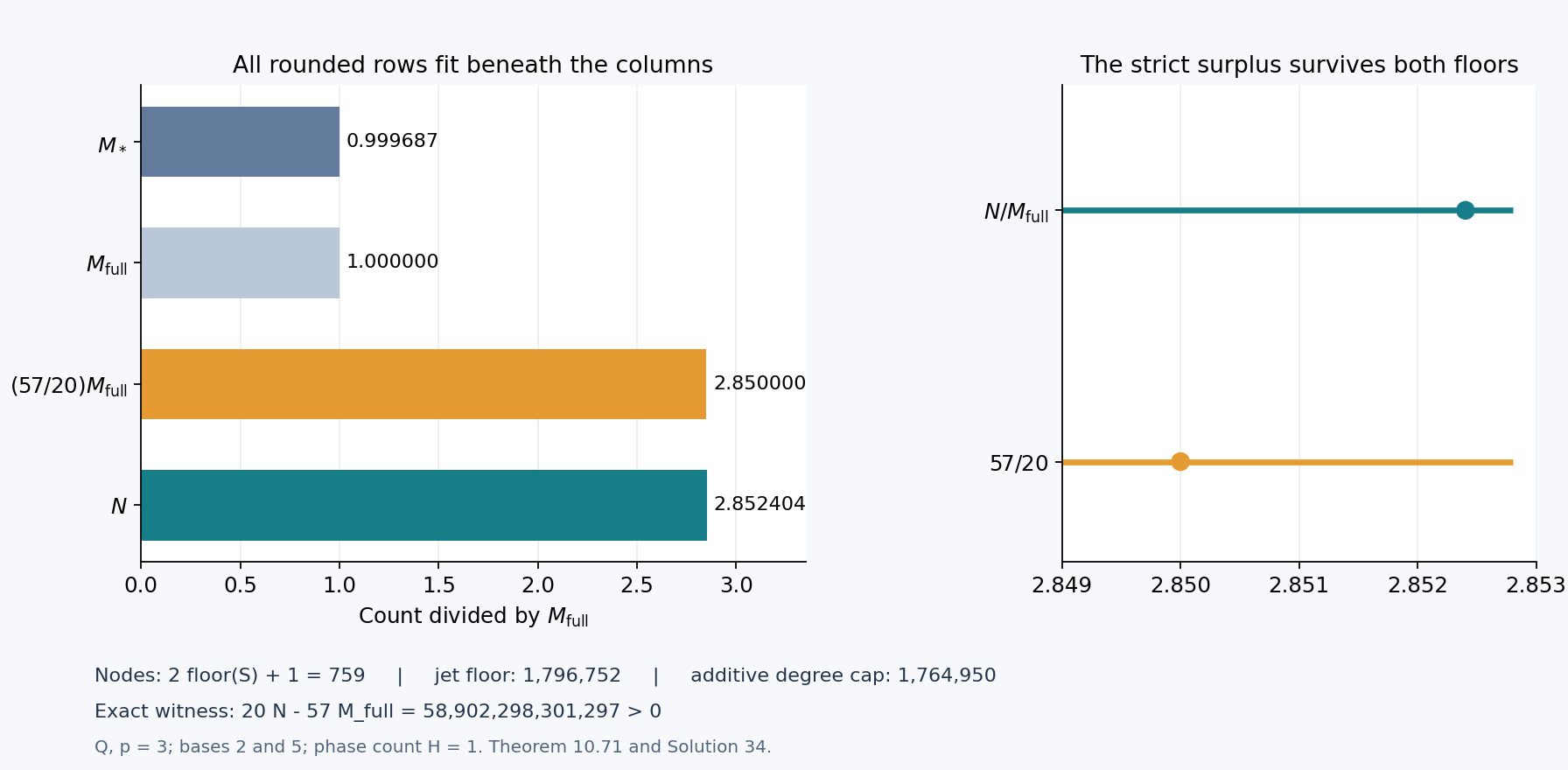
Figure 10.14. Take \(K=\mathbb Q\), \(p=3\), \((\alpha_1,\alpha_2)=(2,5)\), and the parameters in Solution 34. The prepared column count and every plotted comparison are exact integer or rational quantities. There are \(2\lfloor S\rfloor+1\) nodes and \(\binom{\lfloor T\rfloor+2}{2}\) possible jets per node. The surplus \(c_{01}=57/20\) is retained through both floors; the strict comparison follows from the full real parameters, without rounding either budget upwards. The phase count is one, so no support is lost at that step. See (10.187)–(10.191), Solution 34, and Yu's free paper for further reading.
27. The global size and scalar cost of the initial kernel
We now bound the number of coefficients and the size of each scalar row entry at the parameters of Section 26. Two factors need separate care. A prime-to-\(p\) root field is unramified, which strengthens the global degree bound by the ramification index. The additive prepared derivative also contains an lcm clearing factor; that factor contributes to its ordinary absolute value as well as to its integrality.
The degree available above an unramified root field
Lemma 10.73 (the torsion degree divided by ramification). With the notation of (10.183), we have
\[ \frac d e\ge q^{u-1}(q-1). \tag{10.192} \]Proof. Put \(F=\mathbb Q(\zeta_{q^u})\subseteq K\). The cyclotomic Eisenstein proof in p-adic logarithms: power series, heights and the one-logarithm bound, Proposition 9.7 at the prime \(q\), gives \([F:\mathbb Q]=q^{u-1}(q-1)\): irreducibility over \(\mathbb Q_q\) implies irreducibility over \(\mathbb Q\). Since \(q\ne p\), the completion \(F_{\mathfrak q}\) at the prime below \(\mathfrak p\) is unramified over \(\mathbb Q_p\), by the complete prime-to-\(p\) proof in Cyclotomic, quadratic and Kummer extensions of local fields, Proposition 1.1.
Let \(m=[K:F]\), and choose an \(F\)-basis \(b_1,\ldots,b_m\) of \(K\). Inside \(K_{\mathfrak p}\), the subspace \(\sum_jF_{\mathfrak q}b_j\) has dimension at most \(m\) over the complete field \(F_{\mathfrak q}\). It is complete, hence closed, by the finite-dimensional norm proof in Extensions of complete valued fields, Proposition 2.1. It contains \(K\), whose closure is \(K_{\mathfrak p}\), so it equals that completion. Therefore \([K_{\mathfrak p}:F_{\mathfrak q}]\le m\).
Ramification indices multiply in a tower: restriction of a normalized integer valuation multiplies it by the ramification index at each step. The base root field has ramification index one, so \(e=e(K_{\mathfrak p}/F_{\mathfrak q})\). The degree formula \(ef=[L:K]\), fully proved by residue digits in Extensions of complete valued fields, Theorem 3.1, gives \(e\le[K_{\mathfrak p}:F_{\mathfrak q}]\le m\). Therefore \(d/e=[F:\mathbb Q]m/e\ge[F:\mathbb Q]\), as asserted. \(\square\)
A lower volume and an upper coefficient count
Retain all real parameters in (10.183)–(10.186). Set
\[ \begin{aligned} b&=\begin{cases}1,&e=1\text{ and }(p\ge5\text{ or }d=1),\\ g_1^{-1},&\text{otherwise},\end{cases}\\ g_{61}&= 2c_0c_1^{1-r}c_4 \left(\frac q{\widehat\vartheta}\right)^r \frac{(r+1)^r\mathrm e^r}{r!r^r}\, t\,\frac{q-1}{q}\,g_1\,(bg_3)^{r-1},\\ v&=q^\nu D_1\cdots D_r. \end{aligned} \tag{10.193} \]Lemma 10.74 (a uniform lower box volume). We have
\[ v\ge g_{61}>0. \tag{10.194} \]Proof. In the maximum defining \(\mathcal D\), use the second member \((\mathrm e^r/r^r)t\). Substituting one factor of \(\mathcal D\) into \(v\), and using \(\gamma\ge1\), \(1+\epsilon\ge1\), and \(2+g_2^{-1}\ge2\), gives \[ v\ge \frac{2c_0c_1^{1-r}c_4}{q^u} \left(\frac q\theta\right)^r \frac{(r+1)^r\mathrm e^r}{r!r^r}\, t\,\frac d{e^r}\ell_d(A+x)\mathcal D^{r-1}. \] Lemma 10.73 gives \(d/q^u\ge e(q-1)/q\); also \(\ell_d\ge1\) and \(\theta\le\widehat\vartheta\). The remaining factor is \((A+x)(\mathcal D/e)^{r-1}\). In the first case for \(b\), \(e=1\) and \(\mathcal D\ge g_3\). In the other case, the stronger bound in (10.187) and \(A+x\ge e\) give \(\mathcal D/e\ge g_3/g_1\). Since \(A+x\ge g_1\), both cases imply \((A+x)(\mathcal D/e)^{r-1}\ge g_1(bg_3)^{r-1}\). This proves (10.194). \(\square\)
Let \(w_K\) denote the full root-of-unity order, and put
\[ \begin{aligned} g_6&= \rho(1+g_5^{-1})(1+g_{61}^{-1}) \frac{r!\mathrm e^r} {c_1^{r+1}c_4c_2^rP^rw_Kr^{2r}},\\ g_7&=\frac{c_3q(r+1)g_0g_3}{t},\\ g_8&=\frac{\ln g_7+g_1+ \max\{\ln(g_6d/\mathrm e^{g_1}),0\}}{g_7} +\frac r{c_3q(r+1)^2}\frac{\ln g_3}{g_3}. \end{aligned} \tag{10.195} \]Theorem 10.75 (the logarithmic coefficient budget). Suppose \(g_3\ge\mathrm e\) and \(g_7\ge\mathrm e\). For the selected support of Theorem 10.71, \(N=kL|\Lambda|\) and \(Z=S\mathcal D/d\) satisfy
\[ N\le g_6S\mathcal D^{r+1}, \qquad Z\ge g_7,\qquad \ln N\le g_8Z. \tag{10.196} \]Proof. By (10.180), \(|\Lambda|\le v+1\). Also \[ kL\le(1+g_5^{-1})\frac{S\mathcal D}{c_1c_4d(A+x)}. \] Use \(v\ge g_{61}\) to replace \(v+1\) by at most \((1+g_{61}^{-1})v\). The full saturation bound (10.55) gives \[ \frac{q^\nu}{d^{r+1}\prod_i\sigma_i} \le\frac{\rho\ell_dr!\mathrm e^r}{w_Kr^r}. \] For \(d\ge2\), use the same replacement of \(\ln d\) by \(\ell_d\) as in (10.188); for \(d=1\) the formula is exact. Substituting the widths \(D_i\) and \(\ell_d\le g_1\le A+x\) gives the first inequality of (10.196), with exactly \(g_6\).
The formula for \(S\), together with \(h+x\ge g_0\) and \(\mathcal D\ge g_3\), gives \(Z\ge g_7\). Taking logarithms in the first inequality yields \[ \ln N\le\ln(g_6d)+\ln Z+r\ln\mathcal D. \] Put \(C=g_1+\max\{\ln(g_6d/\mathrm e^{g_1}),0\}>0\); then \(\ln(g_6d)\le C\), so \(C/Z\le C/g_7\). The function \(\ln y/y\) decreases for \(y\ge\mathrm e\), because its derivative is \((1-\ln y)/y^2\). Thus \(\ln Z/Z\le\ln g_7/g_7\).
Finally \(h+x\ge(r+1)t\) gives \(S/d\ge c_3q(r+1)^2\), and therefore \[ \frac{r\ln\mathcal D}{Z} \le\frac r{c_3q(r+1)^2}\frac{\ln\mathcal D}{\mathcal D} \le\frac r{c_3q(r+1)^2}\frac{\ln g_3}{g_3}. \] Combining these three bounds proves \(\ln N\le g_8Z\). \(\square\)
The lower hypotheses here have simple sufficient conditions. If \(c_0\ge19/10,c_1\ge7/5,c_3\ge47/100,c_4\ge15/4\), then \(g_3/\!t>21\). Indeed \(a_*\ge7/2\), \(\rho\le58\), \(g_1>5\), and \(r^r(r+1)^r/(r!)^2\ge1\); hence \[ \frac{g_3}{t}> \frac2{58}\frac{19}{10}\frac75\frac{15}4 \left(\frac72\right)^2\,5>21. \] The positive logarithm series in Solution 34 gives \(\ln2>2/3\), so \(t\ge\ln2>2/3\), and \(g_3>14>\mathrm e\). Also \(g_7>(47/100)\cdot2\cdot3\cdot39\cdot21>3>\mathrm e\), where \(\mathrm e<3\) follows by summing its positive series and bounding the tail geometrically.
Retaining the clearing factor and the jet allocation
Write \(s_0=\lfloor S\rfloor,t_0=\lfloor T\rfloor,D_{\mathrm a}=kL\), and \(\mathfrak v=v(k)=\operatorname{lcm}(1,\ldots,k)\). For the \(r-1\) integer Euler forms of the actual prepared system, let \(\Omega_j\) be the maximum of their absolute arguments on the support, and put \[ m=\sum_{j=1}^{r-1}\Omega_j+r-2,\qquad U=\min(D_{\mathrm a},t_0). \tag{10.197} \]
Lemma 10.76 (a complete scalar row bound). The scalar bound in Lemma 10.63 may be taken to be
\[ \mathcal H_0= \left[2\mathrm e\left(\frac{s_0}{k}+2\right)\right]^{D_{\mathrm a}} \max_{0\le u\le U} \left\{\mathfrak v^u \binom{m+t_0-u}{t_0-u}\right\}. \tag{10.198} \]If \(\mathfrak v=1\), a maximizing index is \(u_*=0\). If \(\mathfrak v>1\), one is \[ u_*=\min\left\{U,\, \max\left\{0,t_0-\left\lceil\frac m{\mathfrak v-1}\right\rceil+1\right\}\right\}. \tag{10.199} \]
More sharply, with \(R=s_0+2k\), the scalar bound may be taken to be \[ \mathcal H_{\rm fine}= \frac{R^{D_{\mathrm a}}}{(k!)^L} \max_{0\le u\le U} \left\{\left(\frac{\mathfrak v}{R}\right)^u \binom{D_{\mathrm a}}u \binom{m+t_0-u}{t_0-u}\right\}. \tag{10.200} \] A maximizing index \(\widehat u\) is the first index after all the consecutive increasing steps. A step from \(u\) to \(u+1\), for \(u<U\), is increasing or constant precisely when \[ \mathfrak v(D_{\mathrm a}-u)(t_0-u) \ge R(u+1)(m+t_0-u). \tag{10.201} \] These steps form an initial interval, so an integer binary search finds a maximizing index, with no numerical root approximation.
Proof. For \(0\le a<k\), \(1\le\ell\le L\), write \[ F_{a,\ell}(X)=\frac1{(k!)^\ell} \prod_{j=1}^k(X+a+j)^\ell. \] It has degree \(k\ell\), and every shift \(a+j\) is at most \(2k\). In the divided derivative of order \(u\), choose the \(u\) differentiated linear factors. There are \(\binom{k\ell}{u}\) choices. For \(|s|\le s_0\), each remaining factor has absolute value at most \(s_0+2k\). Thus \[ \left|\frac{F_{a,\ell}^{(u)}(s)}{u!}\right| \le \frac{\binom{k\ell}{u}(s_0+2k)^{k\ell-u}}{(k!)^\ell} \le\left[2\mathrm e\left(\frac{s_0}{k}+2\right)\right]^{D_{\mathrm a}}. \] For the last inequality use \(\binom{k\ell}{u}\le2^{k\ell}\), the positive factor \(s_0+2k\ge1\), and \(\ln(k!)\ge k\ln k-k\). The latter follows by comparing \(\sum_{j=1}^k\ln j\) with the integral of the increasing function \(\ln x\) on \([1,k]\). The resulting base is greater than one, and \(k\ell\le D_{\mathrm a}\). If \(u>k\ell\), the derivative is zero.
The prepared derivative multiplies this divided derivative by \(\mathfrak v^u\), by (10.86); discarding that multiplier would give the wrong ordinary absolute-value bound. Each Euler factor satisfies \[ |\Delta(\omega_j;t_j)| \le\binom{\Omega_j+t_j}{t_j}. \] Multiplying the positive generating series for these binomial coefficients, as in (10.124), shows that their product at total Euler order \(h\) is at most \(\binom{m+h}{h}\). This increases with \(h\), so for additive order \(u\) it is at most \(\binom{m+t_0-u}{t_0-u}\). This proves (10.198).
For \(F(u)=\mathfrak v^u\binom{m+t_0-u}{t_0-u}\), whenever \(u<t_0\), \[ \frac{F(u+1)}{F(u)} =\mathfrak v\frac{t_0-u}{m+t_0-u}. \] At \(\mathfrak v=1\) this is at most one. Otherwise it is at least one exactly when \((\mathfrak v-1)(t_0-u)\ge m\). These ratios decrease as \(u\) increases. Hence \(F\) increases up to this integer threshold and decreases afterwards; equality may give two adjacent maximizers. Clamping the last increasing step to \([0,U]\) gives (10.199), choosing the larger maximizer in the equality case.
For (10.200), retain the first divided-derivative estimate, rather than replacing its binomial coefficient by \(2^{k\ell}\). Since \(\binom{k\ell}{u}\le\binom{D_{\mathrm a}}u\) and \(R^k/k!>1\), it gives \[ \left|\frac{F_{a,\ell}^{(u)}(s)}{u!}\right| \le \binom{D_{\mathrm a}}u\,R^{-u} \left(\frac{R^k}{k!}\right)^\ell \le\frac{\binom{D_{\mathrm a}}u R^{D_{\mathrm a}-u}}{(k!)^L}. \] Multiply by the clearing and Euler factors already proved. The ratio of the resulting expression at \(u+1\) to that at \(u\) is \[ \frac{\mathfrak v}{R}\frac{D_{\mathrm a}-u}{u+1} \frac{t_0-u}{m+t_0-u}. \] Every factor depending on \(u\) decreases on \(0\le u<U\); the first is strictly decreasing. Thus the ratios cross one at most once. Clearing their positive denominators gives exactly (10.201), which proves the asserted integer rule and the sharper bound. \(\square\)
Corollary 10.77 (the normalized additive cost). If \(c_3q/t\le8\), the first factor in (10.198) contributes at most \[ \frac{D_{\mathrm a}}Z \ln\left[2\mathrm e\left(\frac{s_0}{k}+2\right)\right] \le\frac{1+g_5^{-1}}{c_1c_4}. \tag{10.202} \]
Proof. Since \(h+x>39\), \(k=\lfloor h+x\rfloor\ge39\) and \((h+x)/k<(k+1)/k\le40/39\). Put \(W=(r+1)d\ge3\). Then \[ \frac{s_0}{k}+2\le\frac Sk+2 <\frac{320}{39}W+2\le\frac{346}{39}W. \] Since \(\mathrm e^3>18>692/39\), it follows that \(2\mathrm e(s_0/k+2)<\mathrm e^4W\), and its logarithm is at most \(g_1\). The inequality \(\mathrm e^3>18\) follows already from the terms of degrees zero through five in its exponential series at three. Also \(D_{\mathrm a}/Z\le(1+g_5^{-1})/[c_1c_4(A+x)]\), by (10.187), and \(g_1\le A+x\). These prove (10.202). For odd \(p\), the hypothesis holds whenever \(c_3\le4\), since \(\ln p\ge\ln3>1\). At \(p=2\), it holds whenever \(c_3\le1/2\), since \(\ln2>2/3\). \(\square\)
Theorem 10.78 (the initial height with all scalar costs). Assume the hypotheses of Theorems 10.71 and 10.75 and Corollary 10.77. Set \(\Psi=u_*\ln\mathfrak v+\ln\binom{m+t_0-u_*}{t_0-u_*}\). Then the integral initial kernel can be chosen with \[ \begin{aligned} \frac{h_2(\boldsymbol c)}Z\le{}& \frac12g_8+\frac{\ln d_0}{2g_7} +\frac{d_0-1}{c_1c_2S}\\ &+\frac1{c_{01}-1} \left[\frac12g_8+\frac{1+g_5^{-1}}{c_1c_4} +\frac{\Psi}{Z} +\frac{1+1/(2g_2)}{2c_1c_2}\right]. \end{aligned} \tag{10.203} \]
Proof. In (10.191), use \(\ln N/Z\le g_8\), \(Z\ge g_7\), and the exact scalar bound (10.198) at (10.199). Corollary 10.77 bounds its additive first factor; its remaining factor has logarithm exactly \(\Psi\). Substitution proves every term of (10.203). The row-field term may further be bounded by \(1/[c_1c_2c_3q(r+1)^2]\), since \(d_0\le d\) and \(S/d\ge c_3q(r+1)^2\), but its exact vanishing at \(d_0=1\) is preferable there.
More sharply, replace the sum \((1+g_5^{-1})/(c_1c_4)+\Psi/Z\) in (10.203) by \(\ln\mathcal H_{\rm fine}/Z\), evaluated at the exact integer maximizer \(\widehat u\) in (10.201). This follows from the same substitution in (10.191), using (10.200).
This is a height bound for coefficients whose existence has already been proved. An extension of their zeros still requires the stated analytic slopes, derivative precision, arithmetic strict comparisons and final multiplicity contradiction. In particular the lcm and Euler term \(\Psi\) must be retained in each such comparison. \(\square\)
Averaging the derivative orders
Corollary 10.79 (a mean scalar budget). Retain every Euler index, allowing duplicate rows, but omit the identically zero additive orders above \(D_{\mathrm a}\). Define \[ \begin{aligned} J_u&=\binom{t_0-u+r-1}{r-1}\quad(0\le u\le U),& \overline J&=\sum_{u=0}^U J_u,\\ \overline u&=\frac{\sum_{u=0}^UuJ_u}{\overline J},& \overline h&=\frac{r-1}{r}(t_0-\overline u),& \overline M&=(2s_0+1)\overline J. \end{aligned} \tag{10.204} \] Let \(H(z)=-z\ln z-(1-z)\ln(1-z)\), with endpoint values zero, and put \[ \begin{aligned} A_{\rm mean}&=(D_{\mathrm a}-\overline u)\ln R -L\ln(k!)+D_{\mathrm a}H(\overline u/D_{\mathrm a}),\\ E_{\rm mean}&=\begin{cases} \overline h\ln\!\left[\mathrm e(1+m/\overline h)\right],&\overline h>0,\\ 0,&\overline h=0, \end{cases}\\ B_{\rm mean}&=A_{\rm mean}+\overline u\ln\mathfrak v+E_{\rm mean}. \end{aligned} \tag{10.205} \] The mean logarithm of the scalar row bounds is at most \(B_{\rm mean}\), and an integral initial kernel exists with \[ \begin{aligned} \frac{h_2(\boldsymbol c)}Z\le{}& \frac{\tfrac12\ln(Nd_0)}Z+\frac{d_0-1}{c_1c_2S}\\ &+\frac{\overline M}{N-\overline M} \left[\frac{\tfrac12\ln N+B_{\rm mean}}Z +\frac{s_0(s_0+1)} {(2s_0+1)c_1c_2S}\right]. \end{aligned} \tag{10.206} \] Moreover \(\overline u\le t_0/(r+1)\).
Proof. At fixed additive order \(u\), the \(r-1\) Euler indices and their slack coordinate are all the nonnegative integer compositions of \(t_0-u\) into \(r\) parts. Permuting their coordinates is a bijection; the sum of their coordinate averages is \(t_0-u\). Thus their mean total Euler order is \((r-1)(t_0-u)/r\). Weighting by \(J_u\) proves the formula for \(\overline h\).
Without the additive cutoff, all \(r\) derivative coordinates and their slack are the compositions of \(t_0\) into \(r+1\) parts, so the mean additive order is \(t_0/(r+1)\). Removing orders greater than \(U\) can only decrease that mean: each removed order exceeds every retained one. This proves the last assertion.
The sharper additive estimate in the proof of Lemma 10.76 has logarithm at most \[ \ln\binom{D_{\mathrm a}}u+(D_{\mathrm a}-u)\ln R-L\ln(k!). \] For \(0<u<D_{\mathrm a}\), the binomial theorem at \(z=u/D_{\mathrm a}\) gives \(\binom{D_{\mathrm a}}u z^u(1-z)^{D_{\mathrm a}-u}\le1\). Hence \(\ln\binom{D_{\mathrm a}}u\le D_{\mathrm a}H(u/D_{\mathrm a})\), including the endpoints by continuity. The second derivative \(H''(z)=-1/z-1/(1-z)<0\) proves concavity, so averaging gives \(A_{\rm mean}\).
At total Euler order \(h>0\), the factorial integral bound gives \(\ln\binom{m+h}{h}\le h\ln[\mathrm e(1+m/h)]\). The right side extends continuously by zero at \(h=0\). Its second derivative is \(-m^2/[h(m+h)^2]\le0\), so its average is at most \(E_{\rm mean}\); when \(m=0\) it is the linear function \(h\). The clearing multiplier has logarithm \(u\ln\mathfrak v\), whose mean is exactly \(\overline u\ln\mathfrak v\). This proves (10.205).
By (10.190), \(N>c_{01}(2s_0+1)\binom{t_0+r}{r}\ge c_{01}\overline M\), so the completely proved weighted integral Siegel argument of Lemma 10.63 applies to these rows. Duplicate or further zero rows do not increase rank; assigning them the same positive upper scalar bounds preserves that argument. The row field remains \(E_0\), and the torus-row mean remains that of (10.174). Use (10.173) for its full-width and field-generator terms, and substitute the mean scalar bound into the row sum in (10.171). This is (10.206), with the actual ratio \(\overline M/(N-\overline M)\). The nonzero polynomial and every required jet follow as before. \(\square\)
A second way to clear the global rows
Corollary 10.80 (row scaling and an alternative mean bound). Define \[ B_{\rm proj}=(D_{\mathrm a}-\overline u)\ln R +D_{\mathrm a}H(\overline u/D_{\mathrm a})+E_{\rm mean}. \tag{10.207} \] In (10.206), \(B_{\rm mean}\) may be replaced by \[ \min\{B_{\rm mean},B_{\rm proj}\}. \tag{10.208} \] One may also choose the smaller scalar bound separately at each row before averaging.
Proof. At the additive order \(u\), every original prepared row contains the common multiplier \(\mathfrak v^u\). Replace it by the common multiplier \((k!)^L\). This multiplies that entire row by the nonzero rational number \((k!)^L/\mathfrak v^u\), so it preserves its kernel and its coefficient field. Every nonzero row has unchanged projective height; zero rows remain zero. For a nonzero row, the logarithms of the absolute values of that common scalar sum to zero by the normalized product formula proved in Places of number fields in extensions and the product formula, Theorem 5.2.
The divided derivative of \(F_{a,\ell}\) has denominator dividing \((k!)^\ell\). To verify this at every order, its polynomial coefficients have that denominator and divided differentiation multiplies a monomial coefficient by an integer binomial coefficient. At an integer node its denominator still divides \((k!)^\ell\), hence divides \((k!)^L\). The Euler binomials are integers at their integer arguments. Thus the replaced scalar entries are integers, as required for the same finite-place row estimate.
The sharper derivative bound in Lemma 10.76 now gives the archimedean scalar bound \[ \binom{D_{\mathrm a}}u R^{D_{\mathrm a}-u} \binom{m+t_0-u}{t_0-u}. \] The factorial denominator cancels against the new common multiplier. Averaging its logarithm with the concavity arguments of Corollary 10.79 gives \(B_{\rm proj}\). Its coefficient matrix has exactly the same kernel as the original prepared matrix, so the identical weighted Siegel and full-width argument proves (10.206) with this bound. Both bounds therefore apply to the same row heights; choosing their smaller value, globally or row by row, is valid. The original lcm normalization remains available for every later local jet-precision computation. \(\square\)
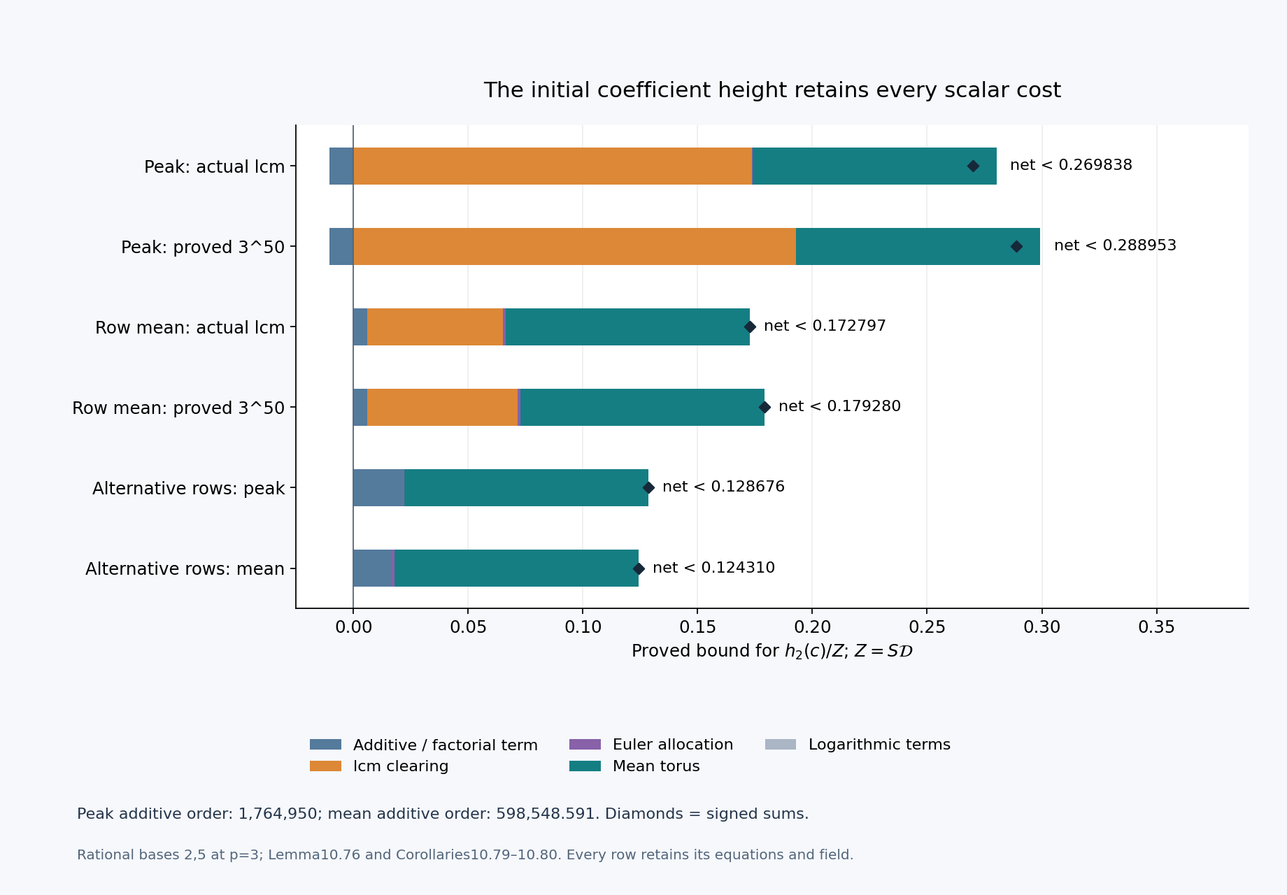
Figure 10.15. The parameters of Solution 34 give the proved coefficient-height bounds in Solution 35. The sharper allocation and row average retain the factorial denominator; lcm clearing, Euler orders, mean torus and logarithmic terms are all included. Left of zero is the factorial contribution to be subtracted when the highest additive order is used. The diamonds mark the net sums. Each pair uses either the actual integer \(\operatorname{lcm}(1,\ldots,50)\) or the completely proved coarser \(3^{50}\) bound in Two logarithms II: explicit lower bounds. The final pair uses the alternative global row clearing of Corollary 10.80. All bars give proved upper bounds on the height of some initial kernel. See (10.198)–(10.208), Solution 35, and Yu's free paper for further reading.
28. Principal-unit depth and the analytic torus
The local torus coordinates must define convergent exponential functions on the enlarged disc used for interpolation. We prove the depth with the same power \(P\) as in Section 26. The ramification index enters this choice; the small strict reduction from \(\vartheta\) to \(\theta\) also has a mathematical purpose.
The power needed for an enlarged disc
Let \(L/\mathbb Q_p\) be a finite extension with ramification index \(e\), and normalize \(v_p(p)=1\). Write \(a_p=1/(p-1)\), and choose the nonnegative integer \(\kappa\) by
\[ p^{\kappa-1}(p-1)\le2e<p^\kappa(p-1),\qquad P=p^\kappa, \qquad \vartheta=\begin{cases} (p-2)/(p-1),&p\ge5, e=1,\\ P/(2e),&\text{otherwise}. \end{cases} \tag{10.209} \]This integer exists: take the least nonnegative \(\kappa\) satisfying the strict upper inequality. At \(\kappa=0\), its lower inequality still holds because \((p-1)/p<1\le2e\). Fix \(0<\theta<\vartheta\); in particular the choice \(\theta=\vartheta/(1+\varepsilon)\) with \(\varepsilon>0\) is permitted.
Lemma 10.81 (the original principal-unit depth). If \(\beta\in L\) and \(v_p(\beta-1)>0\), then
\[ v_p(\beta^P-1)\ge\vartheta+a_p>\theta+a_p. \tag{10.210} \]The statement includes \(\beta^P=1\), with valuation infinity.
Proof. The valuation group of \(L\) is \(e^{-1}\mathbb Z\), by the complete degree-and-residue proof in Extensions of complete valued fields, Theorem 3.1. Thus \(v_p(\beta-1)\ge1/e\). The elementary power step in p-adic logarithms: power series, heights and the one-logarithm bound, Lemma 9.5, gives \(c_{j+1}\ge F(c_j)\) for \(c_j=v_p(\beta^{p^j}-1)\), where \(F(c)=\min\{pc,c+1\}\). Below \(a_p\) the step is exactly multiplication by \(p\); at or above that threshold the lower bound still holds. The function \(F\) is increasing and \(F(c)\ge c\) for \(c\ge0\). If any power is one, all subsequent assertions are immediate.
In the exceptional case \(p\ge5,e=1\), we have \(\kappa=0\), so the initial bound is \(1=\vartheta+a_p\). Consider the other cases. The inequalities defining \(\kappa\) give \(a_p<\vartheta\le p a_p\). If \(\kappa=0\), then \(1/e=2\vartheta>\vartheta+a_p\), which proves the claim.
Suppose \(\kappa\ge1\). We first prove \(c_{\kappa-1}\ge P/(pe)\). If none of \(c_0,\ldots,c_{\kappa-2}\) reaches \(a_p\), the exact steps below the threshold give \(c_{\kappa-1}=p^{\kappa-1}c_0\ge P/(pe)\); for \(\kappa=1\) this uses no step. Otherwise, after the first such crossing there is at least one further step before index \(\kappa-1\). That step gives \(c\ge a_p+1\ge2a_p\). Subsequent steps cannot decrease the valuation, and the lower defining inequality gives \(P/(pe)\le2a_p\). This proves the same bound in that case.
Applying the increasing function \(F\) once more yields
\[ c_\kappa\ge\min\{P/e, 1+P/(pe)\} =\min\{2\vartheta, 1+2\vartheta/p\} \ge\vartheta+a_p. \tag{10.211} \]Indeed \(2\vartheta>\vartheta+a_p\). For the other member, use \((1-2/p)\vartheta\le(p-2)/(p-1)=1-a_p\). This remains valid at \(p=2\), where both sides of that last inequality are zero. Finally \(\theta<\vartheta\) supplies the strict inequality in (10.210). \(\square\)
Coefficients and divided jets of the torus functions
Corollary 10.82 (normality with the actual depth). Let \(w_1,\ldots,w_s\in L\) satisfy \(v_p(w_i-1)\ge\vartheta+a_p\), and let \(\lambda_i\in L\) have \(v_p(\lambda_i)\ge0\). Put
\[ \ell=\sum_i\lambda_i\log w_i,\qquad F(Z)=\exp(Z\ell)=\sum_{n\ge0}A_nZ^n. \tag{10.212} \]Then \(F\in\mathcal A_{p^\theta}\), its Gauss norm is one, and for \(n\ge1\)
\[ v_p(A_n)\ge n\vartheta+a_p,\qquad v_p(A_n)-n\theta\ge n(\vartheta-\theta)+a_p. \tag{10.213} \]If \(v_p(z)\ge-\theta\), its divided jets satisfy
\[ \frac{F^{(j)}(z)}{j!}=F(z)\frac{\ell^j}{j!},\qquad v_p\!\left(\frac{F^{(j)}(z)}{j!}\right) \ge j\vartheta+a_p\quad(j\ge1). \tag{10.214} \]If \(\ell=0\), the positive-order coefficients and jets are zero. The constant coefficient and value have valuation zero.
Proof. The logarithm is an isometry at this depth, by Proposition 9.3 of the linked preceding lesson. Thus each logarithm has valuation at least \(\vartheta+a_p\), and the integral multipliers and ultrametric inequality give the same bound for \(\ell\). If \(\ell=0\), the assertions follow from \(F=1\). Otherwise \(A_n=\ell^n/n!\). The complete factorial digit formula (9.4) gives \(v_p(n!)=(n-s_p(n))a_p\le(n-1)a_p\). This proves the first bound in (10.213); subtracting \(n\theta\) proves the second. It tends to infinity, so the series belongs to the complete coefficient algebra \(\mathcal A_{p^\theta}\). The constant coefficient is one and every other weighted coefficient has positive valuation, proving that the Gauss norm is exactly one.
For the asserted nodes, \(v_p(z\ell)\ge\vartheta-\theta+a_p>a_p\). The exponential converges there and is a unit, by Proposition 9.3. The coefficient algebra and analytic identities of Lemma 9.2 and Proposition 9.4 justify differentiation and translation on this disc; alternatively the coefficient identity for each divided derivative is verified directly by the convergent exponential series. It gives (10.214), with the same factorial estimate. \(\square\)
This applies to the integer exponent vectors of every torus monomial, including negative coordinates, and to exponents divided by any power of \(q\ne p\). Such scalars are p-adically integral. Finite sums of these exponential series with locally integral coefficients have Gauss norm at most one. An additional additive polynomial still contributes its own coefficient norm; (10.213) does not discard that contribution.
The strict choice of \(\theta\) cannot generally be removed. If \(v_p(\ell)=\vartheta+a_p\), then the exact factorial formula gives \(v_p(A_n)-n\vartheta=s_p(n)a_p\). At \(n=p^j\) this is the constant \(a_p\). The weighted coefficients therefore fail to tend to zero at radius \(p^\vartheta\). In this equality case the exponential does not converge at a point of valuation \(-\vartheta\). Solution 36 supplies an actual example.
Residue phases and a coherent root choice
Corollary 10.83 (principal roots of the phased coordinates). Let \(G=p^f-1\), let \(\zeta\in L\) be a primitive \(G\)-th root of unity, and suppose that the residue of the local unit \(\alpha\) is the residue of \(\zeta^a\). Such residue lifts, including their primitivity, are proved in Lemma 10.53. Put
\[ \beta=\alpha\zeta^{-a},\qquad V=\beta^P=\alpha^P\zeta^{-aP}. \tag{10.215} \]For a prime \(q\ne p\), the element
\[ \eta=\exp(q^{-1}\log V)\in L,\qquad \eta^q=V,\qquad v_p(\eta-1)=v_p(V-1)\ge\vartheta+a_p \tag{10.216} \]is the unique \(q\)-th root of \(V\) with residue one. Fix \(\xi\in\mathbb C_p\) with \(\xi^q=\zeta\). A \(q\)-th root \(\rho\) of \(\alpha\) can be chosen so that
\[ \rho^P\xi^{-aP}=\eta. \tag{10.217} \]The choice may be made separately for every member of a finite family, without changing any of their \(q\)-th power identities.
Proof. The residue condition gives \(v_p(\beta-1)>0\). Lemma 10.81 therefore proves the depth of \(V\). Since \(q\) is a local unit, \(q^{-1}\log V\) has this same valuation; Proposition 9.4 gives both \(\eta^q=V\) and the valuation identity. The series defining \(\eta\) lies in the complete field \(L\). If two such roots had residue one, their ratio would be a \(q\)-th root of unity with positive valuation of its difference from one. The prime-to-\(p\) power identity in Lemma 9.5 forces that ratio to be one. This proves uniqueness, also when \(V=1\).
Start with any \(\rho_0^q=\alpha\) in \(\mathbb C_p\). Then \(w=\rho_0^P\xi^{-aP}\) satisfies \(w^q=V\), so \(\eta/w\) is a \(q\)-th root of unity. Fix a primitive one \(\omega\), and write \(\eta/w=\omega^j\). Since \(P=p^\kappa\) is coprime to \(q\), integer division gives an integer \(b\) with \(Pb\equiv j\pmod q\). Set \(\rho=\rho_0\omega^b\). Its \(q\)-th power is still \(\alpha\), and its \(P\)-th power supplies the required correction, proving (10.217). No equation for another member of the family is affected. \(\square\)
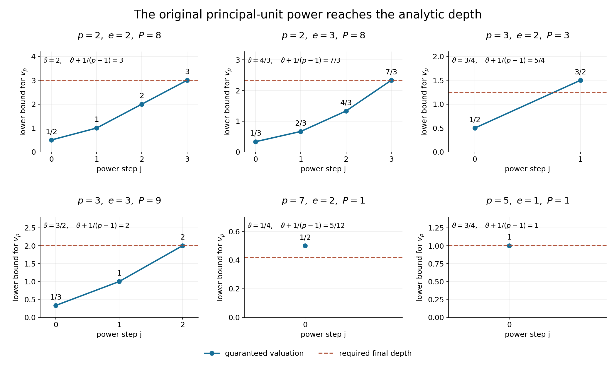
Figure 10.16. Start with the smallest possible positive valuation \(1/e\) and iterate the guaranteed step \(c\mapsto\min\{pc,c+1\}\). The points show lower bounds, not claims that every step is attained by a unit. The horizontal line is the exact final depth \(\vartheta+1/(p-1)\); its special unramified branch is retained at \(p=5,e=1\). The zero-step case \(p=7,e=2\) is included. Lemma 10.81 proves all six bounds and all other ramification cases. Corollary 10.82 then permits every closed radius \(p^\theta\) with \(\theta<\vartheta\). See Solution 36, the figure program, and Yu's free paper, equations (2.1), (4.7) and (4.11), for further reading.
29. The uniform clearing and Euler budget
The saturated coordinates explain the integer arguments of the Euler factors. Their full \(q^\nu\) multiplier matters for ordinary absolute values. Averaging the derivative orders then controls that multiplier and the additive lcm cost together.
Euler arguments in a saturated basis
Let \(\beta_1,\ldots,\beta_n\in K^\times\), with \(n\ge2\) and positive heights \(h_j=h(\beta_j)\). Let \(A_0=(a_{ij})\) be an \(r\)-by-\(n\) integer matrix, \(2\le r\le n\), and suppose that the original independent bases \(\alpha_i\) of Section 26 have the form \(\alpha_i=\zeta_i\prod_j\beta_j^{a_{ij}}\), with roots of unity \(\zeta_i\), and that
\[ \sum_{j=1}^n|a_{ij}|h_j\le\sigma_i,\qquad R_j=\frac{|b_n|}{h_j}+\frac{|b_j|}{h_n}, \qquad R_{\max}=\max_{1\le j<n}R_j. \tag{10.218} \]Here \(b_j\in\mathbb Z\) and \(b_n\ne0\). The product and inverse height inequalities proved earlier give \(h(\alpha_i)\le\sigma_i\), as required in Section 26.
Let \(B\) be a column-basis matrix of the q-primary saturation lattice \(M\supseteq\mathbb Z^r\), of index \(J=q^\nu\). Suppose \(B\Lambda\) lies in a translated closed box of full widths \(D_i\). Fix \(\lambda_0\in\Lambda\), and write \(\mu=B\lambda,\mu_0=B\lambda_0\). For any selected indices \(j<n\), put
\[ \omega_j(\lambda) =J\sum_{i=1}^r(b_na_{ij}-b_ja_{in})(\mu_i-\mu_{0i}). \tag{10.219} \]Lemma 10.84 (the original integer Euler arguments). These are integer linear forms in \(\lambda-\lambda_0\). They are the eigenvalues of \(\sum_i(b_na_{ij}-b_ja_{in})Y_i\partial/\partial Y_i\) on the Laurent monomials \(Y^{J(\mu-\mu_0)}\). With the widths of (10.186),
\[ \Omega_j=\max_{\lambda\in\Lambda}|\omega_j(\lambda)| \le J R_{\max}\sum_iD_i\sigma_i =\frac{q^\nu\mathcal D R_{\max}}{c_1c_2Pd}. \tag{10.220} \]Proof. The quotient \(M/\mathbb Z^r\) has order \(J\). The cyclic subgroup generated by any class has order dividing \(J\), because its distinct cosets partition this finite group into equal-sized sets. Hence \(J\) annihilates every class, and \(JB\) has integer entries. This proves integrality in (10.219). Acting on a Laurent monomial multiplies it by its integer exponent in the differentiated coordinate, which proves the eigenvalue identity, including negative exponents.
Both \(\mu\) and \(\mu_0\) lie in the same translated box, so \(|\mu_i-\mu_{0i}|\le D_i\). No extra factor two is needed for its full widths. Also \[ |b_na_{ij}-b_ja_{in}| \le |b_n||a_{ij}|+|b_j||a_{in}| \le R_j\sigma_i. \] The last inequality uses separately \(|a_{ij}|h_j\le\sigma_i\) and \(|a_{in}|h_n\le\sigma_i\), which follow from (10.218). Sum over \(i\), and substitute \(D_i\sigma_i=\mathcal D/(c_1c_2rPd)\). This gives (10.220). \(\square\)
The same proof divides the bound by \(q^I\) when the full original widths have contracted by \(q^{-I}\). It keeps the original denominator-clearing multiplier \(J\).
The combined mean cost
Use the full composition rows of Corollary 10.79, including duplicate Euler rows, and let \(t_0=\lfloor T\rfloor\ge1\). Retain its \(\overline u,\overline h\), and \(m=\sum_{j=1}^{r-1}\Omega_j+r-2\). Then \(\overline h>0\).
Lemma 10.85 (one budget for clearing and Euler factors). With \(\mathfrak v=\operatorname{lcm}(1,\ldots,k)\), put
\[ \begin{aligned} \mathfrak a_{\rm av} &=\max\left\{\ln\!\left[\mathrm e(1+m/\overline h)\right], \frac12\ln\mathfrak v\right\},\\ E_{\rm mean}+\overline u\ln\mathfrak v &\le t_0\mathfrak a_{\rm av}. \end{aligned} \tag{10.221} \]Proof. The exact composition means in (10.204) give \[ \overline h+2\overline u =\frac{r-1}{r}t_0+\frac{r+1}{r}\overline u \le t_0, \] since \(\overline u\le t_0/(r+1)\). Formula (10.205) bounds the mean Euler logarithm by \(\overline h\ln[\mathrm e(1+m/\overline h)]\); the mean clearing logarithm is exactly \(\overline u\ln\mathfrak v\). Both are bounded by their respective multipliers times \(\mathfrak a_{\rm av}\). Adding proves (10.221). \(\square\)
For the original parameters, we can retain more information than the maximum in this lemma. Define
\[ W(d)=\begin{cases} \ln^3(3d),&d\ge2,\\ \dfrac{\ln6}{\ln2\,\ln3},&d=1, \end{cases} \qquad g_{91}=1+\frac{1+\ln W(d)}{g_0}. \tag{10.222} \]Thus \(g_{91}\) is \(1+(1+3\ln\ln(3d))/g_0\) for \(d\ge2\). Assume in addition to Section 26 that
\[ h\ge\ln\!\left(\frac{R_{\max}}{dW(d)}\right), \qquad c_0\ge19/10,\quad c_4\ge15/4,\quad \widehat\vartheta\le2, \qquad H_1=h+\nu\ln q. \tag{10.223} \]The added height condition is exactly \(R_{\max}\le dW(d)\mathrm e^h\). It is the coefficient-height condition associated with (10.218).
Theorem 10.86 (the original uniform mean Euler budget). Under these assumptions,
\[ \begin{aligned} \frac m{\overline h} &\le\frac47\,\mathrm e^{H_1}tW(d)+\frac{r+1}{t_0},\\ \ln\!\left[\mathrm e(1+m/\overline h)\right] &\le\left(g_{91}+\frac1{2(r-1)}\right)H_1, \end{aligned} \tag{10.224} \]and
\[ E_{\rm mean}+\overline u\ln\mathfrak v \le g_{91}t_0H_1. \tag{10.225} \]Proof. First \(T\ge g_4>9\). To verify the latter lower bound directly, the factor defining \(g_4\) is at least \(g_1^{-1}\). Insert \(g_3\) from (10.185), cancel \(c_1,g_1,t\), and use \(q\ge2,r+1\ge3,\rho\le58,a_*\ge7/2\) and \(r!\le r^r\). This gives \[ g_4\ge\frac62\frac{2(19/10)(15/4)}{58} \left(\frac72\right)^2 =\frac{8379}{928}>9. \] Consequently \(t_0\ge1\) and \(T/t_0<2\).
We have \(\overline h\ge(r-1)t_0/(r+1)\). Sum (10.220), use (10.223), and use \(T=q(r+1)\mathcal D/(c_1\theta et)\). Then \[ \frac m{\overline h} \le\mathrm e^{H_1}\frac{T}{t_0} \frac{\theta e}{P}\frac{tW(d)}{c_2q}+ \frac{(r+1)(r-2)}{(r-1)t_0}. \] Indeed the factor \(d\) in \(R_{\max}\le dW(d)\mathrm e^h\) cancels the global degree in (10.220). Formula (10.184) gives \(\theta e/P\le1\), including its special unramified case, and \(c_2q\ge7/2\). These inequalities prove the first line of (10.224).
Both branches have \(W(d)\ge1\). For \(d\ge2\), \(\ln(3d)\ge\ln6>1\). For \(d=1\), use \(\ln6=\ln2+\ln3\) and \(\ln2<1\), so \(W(d)=1/\ln2+1/\ln3>1\). Since \(t\ge\ln2>2/3\) and \(H_1\ge(r+1)t\), we have \(r+1<3H_1/2\). Moreover \(H_1>39\) implies \[ 1+\frac{3H_1}{2}<\frac3{14}H_1^2 \le\frac37\mathrm e^{H_1}. \] The last inequality follows from the quadratic term of the positive exponential series. This absorbs the \(1+(r+1)/t_0\) term in the first line of (10.224), yielding \[ 1+m/\overline h\le \mathrm e^{H_1}W(d)\max\{t,1\}. \] Take logarithms and add one. As \(H_1\ge g_0\), the constant \(1+\ln W(d)\) is at most \((g_{91}-1)H_1\). The function \(\ln z/z\) has maximum \(1/\mathrm e\) for \(z>0\), by differentiating. Hence \(\ln\max\{t,1\}\le t/\mathrm e\le H_1/[\mathrm e(r+1)]\le H_1/[2(r-1)]\), since \(\mathrm e>2\). This proves the second line of (10.224).
The complete lcm bound in Two logarithms II: explicit lower bounds gives \(\ln\mathfrak v<k\ln3<(3/2)H_1\). Here \(k\le H_1\), and \(\ln3<3/2\) follows already from \(1+3/2+(3/2)^2/2>3\) in the positive exponential series.
Put \(a=g_{91}+1/[2(r-1)]\). We have bounded the combined mean by \[ H_1\left[\frac{r-1}{r}(t_0-\overline u)a+ \frac32\overline u\right]. \] This is affine in \(\overline u\), so its maximum on \([0,t_0/(r+1)]\) occurs at an endpoint. At zero its coefficient of \(t_0H_1\) is \((r-1)g_{91}/r+1/(2r)\le g_{91}\). At the other endpoint that coefficient is \(((r-1)g_{91}+2)/(r+1)\le g_{91}\). Both inequalities use \(g_{91}\ge1\). This proves (10.225). \(\square\)
The full initial coefficient-height bound
Corollary 10.87 (a uniform bound for all initial scalar rows). Assume also the hypotheses of Theorem 10.75 and Corollary 10.77. An integral initial kernel with all required zeros can be chosen with mean scalar logarithm at most
\[ \ln\mathcal B_{\rm av} =kL\ln\!\left[2\mathrm e\left(\frac{s_0}{k}+2\right)\right] +g_{91}TH_1. \tag{10.226} \]In particular
\[ \frac{\ln\mathcal B_{\rm av}}Z \le\frac{1+g_5^{-1}}{c_1c_4} +\frac{g_{91}}{c_1c_3\theta e}. \tag{10.227} \]With \(d_0\) the actual row-field degree, its coefficients satisfy
\[ \begin{aligned} \frac{h_2(\boldsymbol c)}Z\le{}& \frac12g_8+\frac{\ln d_0}{2g_7} +\frac{d_0-1}{c_1c_2S}\\ &+\frac1{c_{01}-1}\left[ \frac12g_8+\frac{1+g_5^{-1}}{c_1c_4} +\frac{g_{91}}{c_1c_3\theta e} +\frac{1+1/(2g_2)}{2c_1c_2}\right]. \end{aligned} \tag{10.228} \]Proof. At every additive order, the first factor of (10.198) bounds its divided derivative before the lcm multiplier. Its logarithm is independent of the derivative allocation, so it also bounds its average. Theorem 10.86 bounds the mean lcm and Euler contributions together by \(g_{91}t_0H_1\le g_{91}TH_1\). This proves (10.226). Corollary 10.77 bounds its first normalized term. The exact parameter formulas give \[ \frac{TH_1}{Z}=\frac1{c_1c_3\theta e}, \] proving (10.227).
Use the full composition rows and their actual ratio \(\overline M/(N-\overline M)\) in (10.206). The column surplus (10.190) bounds that ratio by \(1/(c_{01}-1)\). Insert (10.227), \(\ln N/Z\le g_8\), \(Z\ge g_7\), and the exact mean-node bound from Corollary 10.72. This is (10.228), with every scalar, logarithmic, field-generator and torus cost retained. The row field and the integral nonzero coefficient conclusion are those of Lemma 10.63. \(\square\)
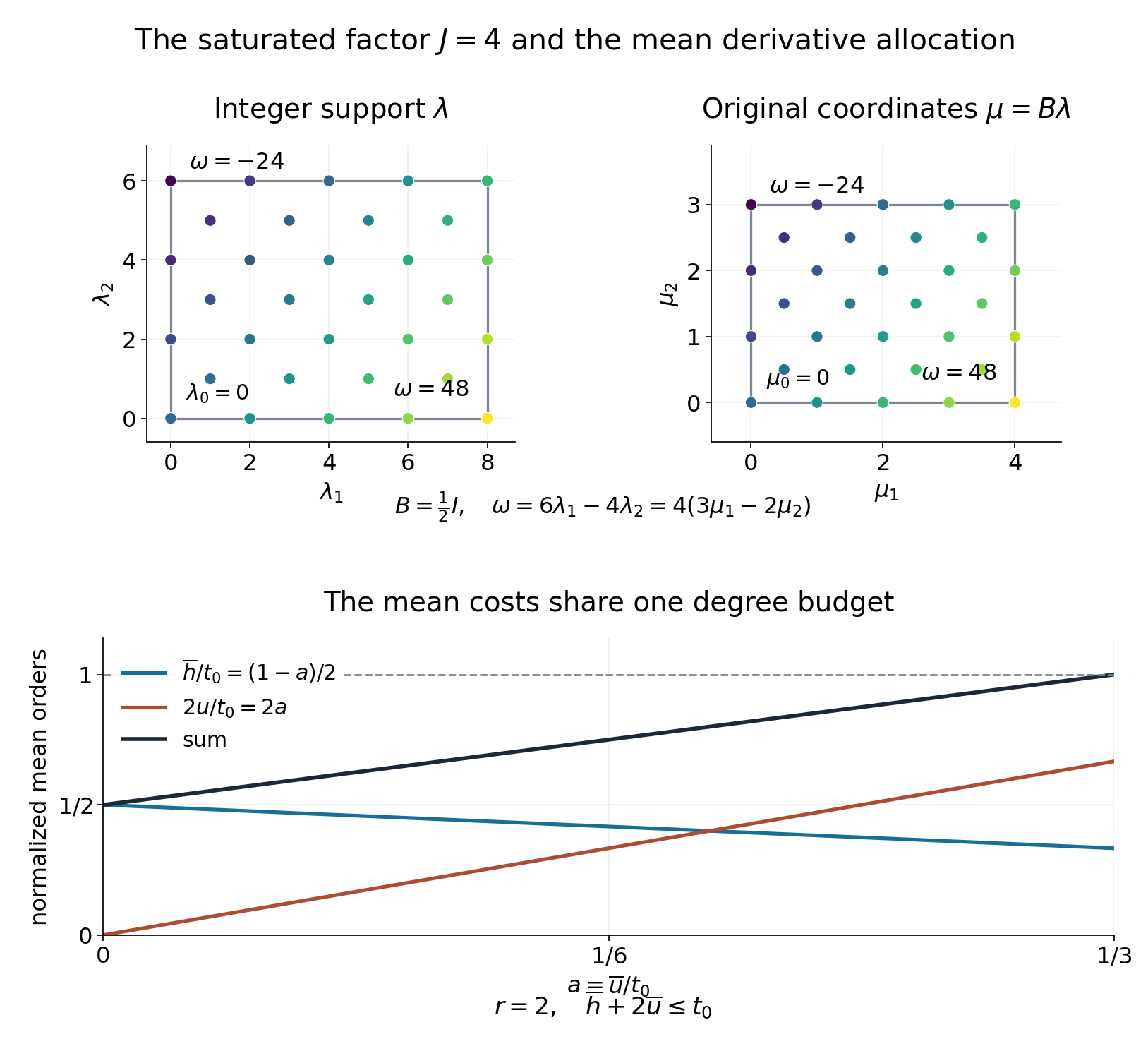
Figure 10.17. Take the rational bases \(4,9\), their q-primary saturated generators \(2,3\), and \(J=4\). The map \(B=\tfrac12I\) sends the integer support on the left to its original coordinates in the upper right panel. Retain the phase class \(\lambda_1+\lambda_2\equiv0\pmod2\). With \((b_1,b_2)=(2,3)\), the prepared Euler argument is \(6\lambda_1-4\lambda_2=4(3\mu_1-2\mu_2)\). Its extrema at the reference \(\lambda_0=0\) are \(48\) and \(-24\), marked at the corresponding vertices. The lower panel shows the exact mean relation at \(r=2\): for \(a=\overline u/t_0\le1/3\), the normalized Euler mean is \((1-a)/2\) and their weighted sum \((1-a)/2+2a\) is at most one. Lemma 10.84 keeps the full clearing factor and original widths; Lemma 10.85 and Theorem 10.86 control the cost after averaging orders. The coordinates and values are reconstructed in Solution 37. Figure program. Human-source context: Yu's free paper, equations (2.8), (4.23) and (5.6).
30. The generator field and its uniform discriminant cost
The initial scalar bound is now uniform. We next control the field in which its coefficients are chosen. A large entry of a saturation basis can make its displayed generators have large heights while leaving the field unchanged. Centering the basis removes that loss. We then use the height-product theorem separately after each omission; the cancellation in \(S\mathcal D/d\) keeps its bound independent of the saturation index.
A centered basis with small generator heights
Lemma 10.88 (a centered saturation basis). Let \(r\ge2\), and let \(M\supseteq\mathbb Z^r\) be a rational lattice of finite index \(J\). Suppose its basis \(B\) corresponds to generators \(\theta_1,\ldots,\theta_r\in K^\times\) in the independent original bases \(\alpha_1,\ldots,\alpha_r\), up to roots of unity. Put \(\sigma_{\max}=\max_i\sigma_i\), where \(h(\alpha_i)\le\sigma_i\).
There is a basis \(B'=BU\), with \(U\in\operatorname{GL}_r(\mathbb Z)\), that is upper triangular and has the following alternatives for each column:
\[ \begin{gathered} B'_{ii}=1\quad\Longrightarrow\quad B'_i=e_i,\\ 0<B'_{ii}<1\quad\Longrightarrow\quad B'_{ii}\le\tfrac12,\qquad |B'_{ji}|\le\tfrac12\quad(j<i),\qquad B'_{ji}=0\quad(j>i). \end{gathered} \tag{10.229} \]Choose \(\theta'_j=\prod_i\theta_i^{U_{ij}}\). Then
\[ \begin{aligned} h(\theta'_j)&\le\sum_i|B'_{ij}|h(\alpha_i) \le\frac r2\sigma_{\max},\\ E&=\mathbb Q(\alpha_0,\theta_1,\ldots,\theta_r) =\mathbb Q(\alpha_0,\theta'_1,\ldots,\theta'_r), \end{aligned} \tag{10.230} \]for any root of unity \(\alpha_0\). This change preserves every normalized monomial, phase class, original support width and integer Euler argument after relabelling \(\lambda'=U^{-1}\lambda\).
Proof. The cyclic-subgroup coset argument in Lemma 10.84 shows that \(J\) kills \(M/\mathbb Z^r\). Thus \(L=JM\) is an integer lattice containing \(J\mathbb Z^r\). Let \(L_i=L\cap\operatorname{span}(e_1,\ldots,e_i)\). Its i-th coordinate image is a nonzero subgroup \(h_i\mathbb Z\) containing \(J\mathbb Z\). Hence \(h_i\) is a positive divisor of \(J\).
Inductively choose \(v_i\in L_i\) whose i-th coordinate is \(h_i\). If \(h_i=J\), choose \(v_i=Je_i\), which belongs to \(L\). Otherwise, subtract integer multiples of \(v_{i-1},\ldots,v_1\), in that descending order, to place coordinate \(j<i\) in the interval \([-h_j/2,h_j/2]\). Ordinary integer division, with either consistent choice at a midpoint, makes this possible. Subtracting \(v_j\) does not change a coordinate larger than \(j\).
The vectors \(v_1,\ldots,v_i\) form a basis of \(L_i\). Indeed, for \(x\in L_i\), subtract the multiple of \(v_i\) specified by its i-th coordinate to obtain an element of \(L_{i-1}\), and use induction. Reading the largest coordinate proves independence. Thus \(B'=(v_1,\ldots,v_r)/J\) is a basis of \(M\). Its diagonal lies in \((0,1]\); a proper divisor \(h_i<J\) is at most \(J/2\). Every centered upper entry has absolute value at most \(h_j/(2J)\le1/2\). The special choice at \(h_i=J\) gives the first alternative in (10.229).
Both \(B\) and \(B'\) are integer bases of the same lattice, so expressing one in the other gives inverse integer matrices \(U,U^{-1}\). The chosen new generators and their inverse products therefore generate exactly the same field. Clear the denominators of \(B'\) and the finite root-of-unity factors by a common positive power. The height product inequality and exact power identity, already proved in the earlier height lesson, give the first inequality of (10.230). A proper-diagonal column has at most \(r\) entries of absolute value at most \(1/2\). A unit column gives height at most \(\sigma_{\max}\le r\sigma_{\max}/2\). This proves the second inequality.
Finally \(B'\lambda'=B\lambda\) and \((\theta')^{\lambda'}=\theta^\lambda\). With the phase vector transformed to \(d'=U^{\mathsf T}d\), we have \(d'\cdot\lambda'=d\cdot\lambda\). Original-coordinate differences, hence their full-width bounds and the integer Euler forms in (10.219), are unchanged. Taking the same integer products of chosen q-th roots also preserves their powers and generated root field; the inverse products recover the old roots. The uniqueness assertion in Corollary 10.83 preserves the principal root choices. \(\square\)
The unit-column alternative matters. Centering only the off-diagonal entries of a column with diagonal one would give the weaker \((r+1)\sigma_{\max}/2\). Choosing the coordinate unit vector avoids this extra half-height.
Each omitted height product and the exact scale
Retain all parameters in (10.183)–(10.186). Write \(w_K\) for the full root-of-unity order, and define
\[ \begin{aligned} g_{11}&=\frac{4q\mathrm e}{\rho}\, c_0c_1c_3c_4a_*^r \frac{(r+1)^{r+1}(r-1)^{r-1}}{(r!)^2}g_0g_1,\\ g_{12}&=\begin{cases} g_1/(2g_7)+1/g_{11},&d\ge2,\\ 0,&d=1. \end{cases} \end{aligned} \tag{10.231} \]These are the original constants in Yu's equation (3.16); \(\mathrm e=\exp(1)\) is distinct from the ramification index.
Lemma 10.89 (the original omitted-product bound). For \(Z=S\mathcal D/d\) and every \(i=1,\ldots,r\),
\[ \begin{gathered} d^r\ell_d\prod_{j\ne i}\sigma_j \ge\frac{w_K}{\rho} \frac{(r-1)^{r-1}}{(r-1)!\,\mathrm e^{r-1}},\\ \frac{2Z}{rd\sigma_i}\ge g_{11}. \end{gathered} \tag{10.232} \]Proof. Every subset of an independent multiplicative family is independent: a relation in that subset would extend by zero exponents to a relation in the full family. Apply the completely proved height-product inequality (10.57) to the \(r-1\) original bases other than \(\alpha_i\). Since \(\sigma_j\ge h(\alpha_j)\), replacing the heights preserves its lower bound. At \(d\ge2\), multiply by \(d^r\ell_d\) and use \(\ell_d\ge\ln d\). At \(d=1\), the proved constant is \(17=\rho\). This proves the first line of (10.232) for each omission separately.
For clarity the exact cancellation in the scale is
\[ \begin{aligned} Z={}&\frac{c_3q(r+1)hA}{q^ut} (1+\epsilon)(2+g_2^{-1})c_0c_1c_4 \left(\frac{c_2qPr(r+1)}{e\theta}\right)^r\frac1{r!}\\ &\quad{}\times \max\left\{\frac{p^f}{\delta t^r}, \frac{\mathrm e^r}{r^r}t\right\} d^{r+1}\ell_d\prod_j\sigma_j. \end{aligned} \tag{10.233} \]It follows by substituting \(S\) and \(\gamma\) in (10.186): the factors \(q^\nu\), \(h+x\) and \(A+x\) cancel exactly. Use \(h\ge g_0\), \(A\ge g_1\), \((1+\epsilon)(2+g_2^{-1})\ge2\), \(c_2qP/(e\theta)\ge a_*\), and the second member of the maximum. We obtain
\[ Z\ge \frac{2q\mathrm e^r}{q^u} c_0c_1c_3c_4a_*^r \frac{(r+1)^{r+1}}{r!}g_0g_1 d^{r+1}\ell_d\prod_j\sigma_j. \]Divide by \(\sigma_i\), insert the first line of (10.232), and use \(w_K\ge q^u\). Multiplication by \(2/(rd)\), together with \(r(r-1)!=r!\), gives exactly \(g_{11}\) in (10.231). No bound on \(q^\nu\) has been inferred from an omitted product. \(\square\)
A uniform coefficient-field and initial height bound
Theorem 10.90 (the original field cost). Let \(E=\mathbb Q(\alpha_0,\theta_1,\ldots,\theta_r)\subseteq K\) be the generator field of the normalized initial rows, and let \(d_E=[E:\mathbb Q]\). Then
\[ \frac{\ln|\Delta_E|}{2d_EZ}\le g_{12}. \tag{10.234} \]Under the remaining hypotheses of Corollary 10.87, the initial rows have a nonzero integral kernel \(c\in\mathcal O_E^N\subseteq\mathcal O_K^N\) giving every original zero and the same nonzero-polynomial conclusion, with
\[ \begin{aligned} \frac{h_2(c)}Z\le{}& g_{12}+\frac{g_8}{2}\\ &+\frac1{c_{01}-1}\left[ \frac{g_8}{2} +\frac{1+g_5^{-1}}{c_1c_4} +\frac{g_{91}}{c_1c_3\theta e} +\frac{1+(2g_2)^{-1}}{2c_1c_2}\right]. \end{aligned} \tag{10.235} \]Proof. At \(d=1\), \(E=\mathbb Q\) and its discriminant is one. Suppose \(d\ge2\), and use the centered generators of Lemma 10.88. Apply the complete discriminant-and-generators argument (8.33) in Linear forms in many logarithms to the tower obtained by first adjoining \(\alpha_0\), then the \(\theta'_j\). The first height is zero. The product of its nontrivial degrees is \(d_E\); induction on \((a-1)+(b-1)\le ab-1\) bounds the sum of the degree decrements by \(d_E-1\). Consequently
\[ \frac{\ln|\Delta_E|}{2d_E} \le\frac{\ln d_E}{2} +(d_E-1)\frac r2\sigma_{\max}. \tag{10.236} \]Choose an index attaining \(\sigma_{\max}\). Lemma 10.89 gives \(r\sigma_{\max}/2\le Z/(dg_{11})\). Since \(d_E\le d\), the second term in (10.236), divided by \(Z\), is at most \((d_E-1)/(dg_{11})<1/g_{11}\). Also \(Z\ge g_7\) and \(\ln d_E\le\ln d<g_1\), so its first term is at most \(g_1/(2g_7)\). This proves (10.234), with the original \(g_{12}\).
Every initial row entry is its integer prepared scalar times \(\alpha_0^{sw_\lambda}\theta^{Ps(\lambda-\lambda_0)}\), by (10.151), hence belongs to \(E\). Apply the complete weighted integral Siegel proof (8.40) over this field, allowing the full composition rows and retaining zero or duplicate rows as in Theorem 10.79. Their normalized heights do not change upon restriction to \(E\), by the field-invariance argument in Theorem 10.59. The resulting bound is the original row-sum inequality with discriminant term \(\ln|\Delta_E|/(2d_E)\).
Insert (10.234), \(\ln N/Z\le g_8\), the exact row ratio bounded by \(1/(c_{01}-1)\), the mean scalar bound (10.227), and the mean-node torus term in Corollary 10.72. This is (10.235). The vector is integral over \(E\), hence over \(K\); it is nonzero, and Lemma 10.29 gives the nonzero Laurent polynomial. The representative-row identities used in Theorem 10.55 supply every original jet zero. \(\square\)
The field bound uses the same \(g_{12}\) as the original argument. Equation (10.235) retains the complete mean scalar budget proved with \(\operatorname{lcm}(1,\ldots,k)<3^k\). A later individual prepared value still has its own scalar, denominator and field costs; averaging the initial rows does not change that value.
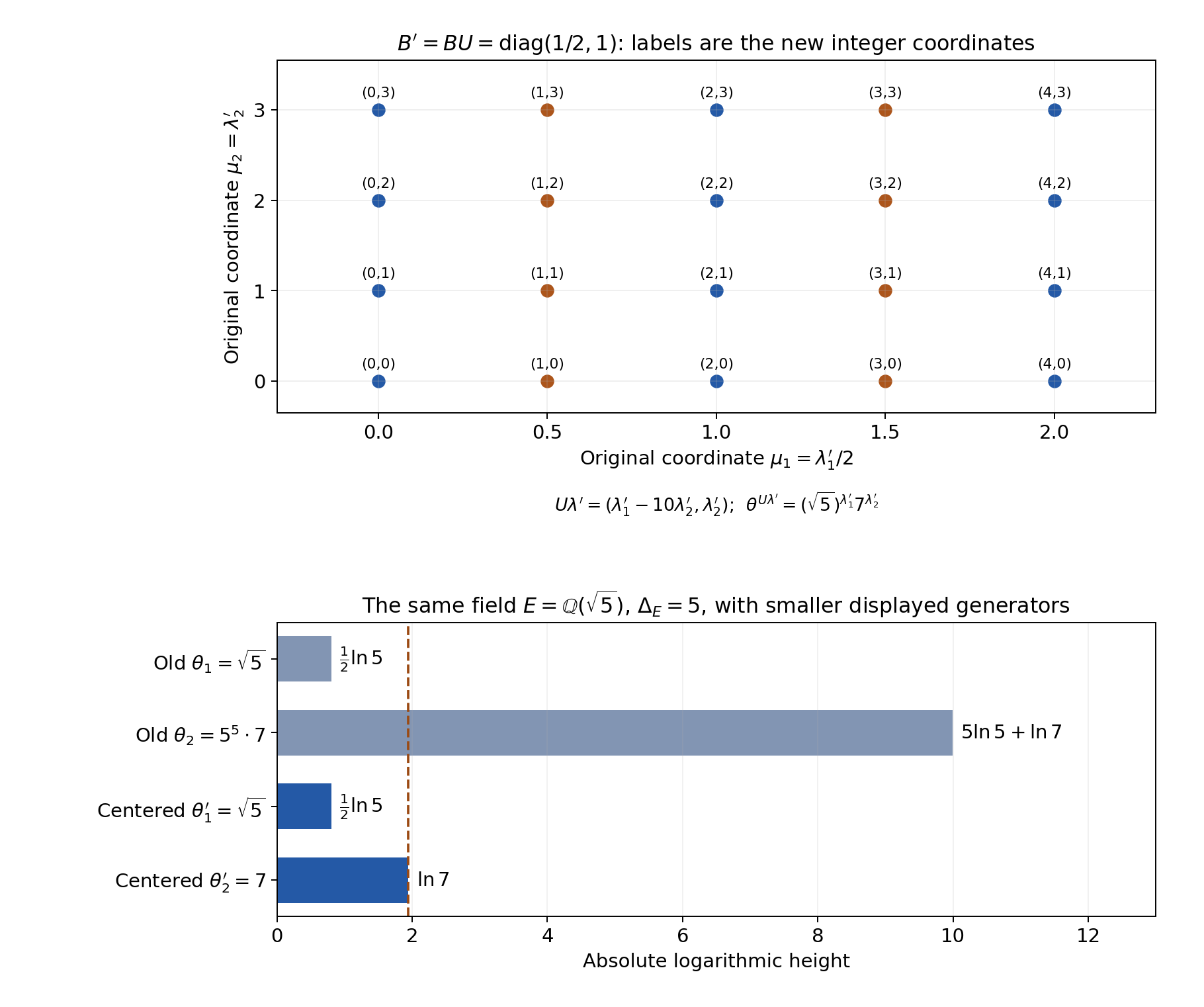
Figure 10.18. Over \(K=\mathbb Q(\sqrt5)\), the original bases \(5,7\) have saturation lattice \((\tfrac12\mathbb Z)\times\mathbb Z\) and index two. The displayed basis \(B=\left(\begin{smallmatrix}1/2&5\\0&1\end{smallmatrix}\right)\) has generators \(\sqrt5,5^5\cdot7\). The integer matrix \(U=\left(\begin{smallmatrix}1&-10\\0&1\end{smallmatrix}\right)\) gives \(B'=BU=\operatorname{diag}(1/2,1)\) and generators \(\sqrt5,7\). The sampled lattice points, blue for an even first coordinate and brown for an odd one, are labelled by \(\lambda'\), with original coordinates \(B'\lambda'=(\lambda'_1/2,\lambda'_2)\). In the old basis they have labels \(U\lambda'\), producing exactly the same points and monomials. The height bars are numerical renderings of the labelled exact logarithms; the dashed line is the centered bound \(r\sigma_{\max}/2=\ln7\). Both lists generate the same quadratic field of discriminant five. Lemmas 10.88–10.89 and Theorem 10.90 prove the basis, omitted-product and field-budget mechanisms; Solution 38 checks this example and the normalized original constants. Figure program. Human-source context: Yu's free paper, equations (3.16), (3.23) and Lemma 4.2; Loher and Masser's free paper, Theorem 3, whose complete height-product proof is given in Section 9.
31. Individual scalar values and a complete integer extension
The initial coefficient estimate averages its rows. An individual value in the induction has its own additive order, ordinary absolute value and denominator. We retain these costs together with the actual derivative precision. At the end of this section, all three integer extensions of the original rational rank-two parameter example are verified uniformly over its permitted coefficient family.
The actual projected slopes and the additive order
Lemma 10.91 (normality at the original logarithmic slopes). Let \(q\ne p\), \(\nu\ge0\), \(A_0=(a_{ij})\) an integer \(r\)-by-\(n\) matrix, and \(b_1,\ldots,b_n\in\mathbb Z\) with \(b_n\ne0\) and \(v_p(b_j)\ge v_p(b_n)\). Suppose \(z_j\in\mathbb C_p\) satisfy \(v_p(z_j)\ge\vartheta+1/(p-1)\), and \(0<\theta<\vartheta\). Put
\[ \begin{aligned} u_i&=q^{-\nu}\sum_{j=1}^na_{ij}z_j,& \mathcal L&=\sum_jb_jz_j,\\ w_i&=u_i-\frac{q^{-\nu}a_{in}}{b_n}\mathcal L =q^{-\nu}\sum_{j<n} \left(a_{ij}-\frac{b_j}{b_n}a_{in}\right)z_j. \end{aligned} \tag{10.237} \]Every \(u_i,w_i\) has valuation at least \(\vartheta+1/(p-1)>\theta+1/(p-1)\), with the convention \(v_p(0)=\infty\). Thus the normality hypotheses of Proposition 10.37 hold for the original and projected curves.
More precisely, retain its prepared family, \(\rho,c_*,\delta,k,L\), and let \(D_{\mathrm a}=kL\), \(\mathfrak v=\operatorname{lcm}(1,\ldots,k)\). For a fixed additive order \(u=t_0\le D_{\mathrm a}\), the following function is normal:
\[ \begin{aligned} F_u(Z;\boldsymbol t) &=\frac{\rho^{D_{\mathrm a}-u}(k!)^L} {c_*\mathfrak v^u}\,f(Z/\rho;\boldsymbol t),\\ G_u&=(D_{\mathrm a}-u)\theta+Lv_p(k!) -u v_p(\mathfrak v),\\ v_p\!\left(\frac{\rho^{D_{\mathrm a}-u}(k!)^L} {c_*\mathfrak v^u}\right)&=G_u-\delta . \end{aligned} \tag{10.238} \]Its ordinary divided jets obey the chain-rule identity (10.107) with scale \(G_u-\delta\). For \(u>D_{\mathrm a}\), every prepared value is zero.
Proof. The fractions \(b_j/b_n\) are p-integral by their valuation hypothesis; \(q^{-\nu}\) is a local unit. Every displayed linear combination therefore has the asserted lower valuation, by the ultrametric inequality. In particular the projected slope does not lose \(v_p(b_n)\): the factors of \(b_n\) have already canceled in (10.237). The principal-unit depth proof in Lemma 10.81 and its logarithmic consequence in Corollary 10.82 supply these \(z_j\) when the original local units are used.
For the scale, the additive factor of a term is the coefficient of \(V^u\) in \[ \frac1{(k!)^\ell} \prod_{a=1}^k(q^{-I}Z/\rho+\lambda_{-1}+a+\mathfrak v V)^\ell, \qquad 1\le\ell\le L,\quad 0\le\lambda_{-1}<k. \] Factoring \(\mathfrak v^u\) from that coefficient leaves an integer-coefficient polynomial in \(q^{-I}Z/\rho\), divided by \((k!)^\ell\), of degree at most \(k\ell-u\). Multiplication by the factor in (10.238) makes every coefficient p-integral: \(q\) is a local unit, \(k\ell-u\le D_{\mathrm a}-u\), and \(\ell\le L\). The ratios \(c_j/c_*\) are p-integral and the integer Euler factors introduce no denominator.
Every exponential factor has argument \(\beta Z/\rho\), where \(\beta\) is an integer linear combination of the \(w_i\). Its positive-degree coefficients tend to zero and have positive valuation, by Corollary 10.82. Its Gauss norm is one. Multiplication by the normalized polynomial, followed by the finite sum over the support, proves normality through Lemma 9.2. The chain rule proves the jet identity. The degree bound proves the final zero assertion. \(\square\)
The scale in (10.238) is allowed to have negative valuation; the prepared derivative already has the compensating local divisibility. The order-independent scale \(G_0-\delta\) remains valid, as proved in Proposition 10.37. We use that common scale in the numerical extension below.
A factorial-preserving pointwise majorant
Take a support at contraction depth \(I\), and let \(\Omega_j\) be nonnegative integer bounds for its \(r-1\) integer Euler arguments. For \(|x|\le X\), define
\[ R_I=q^{-I}X+2k-1,\qquad m_I=\sum_{j=1}^{r-1}\Omega_j+r-2,\qquad D_{\mathrm a}=kL. \tag{10.239} \]Theorem 10.92 (the individual scalar and denominator budget). For a prepared index with additive order \(u\le D_{\mathrm a}\) and Euler order \(h=\sum_{j>0}t_j\), its rational scalar has ordinary absolute value at most
\[ \mathcal H_{I,u,h}(X)= \frac{R_I^{D_{\mathrm a}-u}}{(k!)^L} \mathfrak v^u\binom{D_{\mathrm a}}u \binom{m_I+h}{h}. \tag{10.240} \]Uniformly through total order \(T'\), its scalar bound is
\[ \mathcal H_I^{\rm fine}(X,T')= \frac{R_I^{D_{\mathrm a}}}{(k!)^L} \max_{0\le u\le\min(D_{\mathrm a},T')} \left\{\left(\frac{\mathfrak v}{R_I}\right)^u \binom{D_{\mathrm a}}u\binom{m_I+T'-u}{T'-u}\right\}. \tag{10.241} \]A maximizing index is the first one after all consecutive increasing or constant steps. For \(u<\min(D_{\mathrm a},T')\), their exact test is
\[ \mathfrak v(D_{\mathrm a}-u)(T'-u) \ge R_I(u+1)(m_I+T'-u). \tag{10.242} \]At \(x=s/q^J\), \(s\in\mathbb Z\), all scalar denominators divide \(q^{\Xi_{I,J,u}}\), where
\[ \Xi_{I,J,u}= \begin{cases} 0,&I+J=0,\\ \max\{0,(I+J)(D_{\mathrm a}-u)+Lv_q(k!)-u v_q(\mathfrak v)\}, &I+J>0. \end{cases} \tag{10.243} \]Suppose the normalized torus support has original full widths \(q^{-I}D_i\), \(h(\alpha_i)\le\sigma_i\), and the phase hypotheses of Theorem 10.55. Let the actual algebraic value \(V\) belong to a number field \(F\), with degree \(d_F\) and chosen local degrees \(e_F,f_F\). Its torus monomials are local units and arise from the consistent roots at \(x=s/q^J\). If \(V\ne0\), then
\[ \begin{aligned} v_p(V)-\delta\le\frac{d_F}{e_Ff_F\ln p}\biggl[ &h_2(c)+\tfrac12\ln N+\ln\mathcal H_{I,u,h}(X)\\ &+\Xi_{I,J,u}\ln q +P Xq^{-I}\sum_iD_i\sigma_i\biggr]. \end{aligned} \tag{10.244} \]The field factor is retained even when these roots lie in the old completion.
Proof. Differentiate the product of \(k\ell\) linear factors at \(q^{-I}x+\lambda_{-1}\), dividing by \(u!\). Choosing the \(u\) differentiated factors gives \(\binom{k\ell}u\) terms. Every remaining factor has ordinary absolute value at most \(R_I\), since \(\lambda_{-1}\le k-1\) and \(a\le k\). Multiply by \(\mathfrak v^u\), retaining the denominator \((k!)^\ell\).
If \(u>k\ell\), the derivative is zero. Otherwise \(\binom{k\ell}u\le\binom{D_{\mathrm a}}u\) and \[ \frac{R_I^{k\ell-u}}{(k!)^\ell} =R_I^{-u}\left(\frac{R_I^k}{k!}\right)^\ell \le\frac{R_I^{D_{\mathrm a}-u}}{(k!)^L}, \] because \(R_I\ge k\) makes the parenthesized base at least one. The proved integer Euler generating-series estimate in Lemma 10.76 bounds their product at order \(h\) by \(\binom{m_I+h}h\). This proves (10.240). It increases with \(h\), so maximizing through \(u+h\le T'\) gives (10.241).
The ratio of consecutive terms inside this maximum is \[ \frac{\mathfrak v}{R_I} \frac{D_{\mathrm a}-u}{u+1} \frac{T'-u}{m_I+T'-u}. \] Both variable factors are nonincreasing, and the first strictly decreases. At \(m_I=0\), the last factor is one wherever a step is taken; the terminal value has Euler binomial one. Thus (10.242) describes an initial interval of steps, including this endpoint case. For rational \(R_I\), integer division after clearing its denominator gives an exact binary search.
The scalar is integral at every prime other than \(q\), by the fractional-node argument of Lemma 10.28. At \(q\), the polynomial divided derivative has denominator dividing \((k!)^\ell\) and degree at most \(k\ell-u\). Evaluation at \(q^{-I-J}s+\lambda_{-1}\) costs at most \((I+J)(k\ell-u)\); its multiplier \(\mathfrak v^u\) recovers \(u v_q(\mathfrak v)\). Taking \(\ell\le L\) proves (10.243), with the globally integral \(I+J=0\) case stated separately.
Apply the completely proved nonzero-value product formula of Theorem 10.41 over \(F\), dividing by a coefficient of minimum valuation \(\delta\). Cauchy–Schwarz gives \(h_2(c)+\frac12\ln N\). The scalar bounds just proved give its archimedean and q-denominator terms. The full-width support proof in Theorem 10.64, with contraction as in Theorem 10.60, bounds the torus contribution by \(PXq^{-I}\sum_iD_i\sigma_i\). Taking consistent roots divides heights by \(q^J\), while the node numerator multiplies them by \(|s|\le q^JX\); these two factors cancel. The phase factors have height zero. Summing the place contributions and dividing by \(e_Ff_F\ln p\) gives (10.244). \(\square\)
All three first integer extensions in the rational parameter family
Theorem 10.93 (a complete rank-two integer block). Use the original rational parameters and support of Solution 34, with bases \(2,5\) at three. Let \(b_1,b_2\ne0\) be integers satisfying
\[ \begin{gathered} v_3(b_2)\le v_3(b_1),\qquad R_{\max}=\frac{|b_2|}{\ln2}+\frac{|b_1|}{\ln5} \le W\exp(h),\qquad W=\frac{\ln6}{\ln2\,\ln3},\quad h=g_0,\\ \eta=1-\frac{0.538}{3}=\frac{1231}{1500}, \qquad U=\frac{8Z}{\ln3},\qquad Z=S\mathcal D . \end{gathered} \tag{10.245} \]Choose the integral initial kernel of Theorem 10.90 for this support and these Euler arguments. Assume \(v_3(2^{b_1}5^{b_2}-1)\ge U\). Then the same prepared auxiliary family, without contraction of its support, satisfies
\[ \Phi_0(s;\boldsymbol t)=0 \quad\text{for }|s|\le\lfloor2^jS\rfloor,\quad |\boldsymbol t|\le\lfloor\eta^jT\rfloor,\qquad j=1,2,3. \tag{10.246} \]The allowed coefficient family in (10.245), rather than one chosen pair \(b_1,b_2\), is covered by these comparisons.
Proof. Put \(\beta_1=-2,\beta_2=-5\), both in \(1+3\mathbb Z_3\), and \(u_i=\log(\beta_i^3)\). Since \(\beta_1^3-1=-9\) and \(\beta_2^3-1=-126\), the exact logarithm valuation identity in Proposition 9.3 gives \(v_3(u_i)=2\). Here \(\nu=0\), \(P=3\), and \(\theta<3/2\). The hypothesis on the multiplicative difference forces \(b_1+b_2\) even by reduction modulo three. Hence \(\mathcal L=b_1u_1+b_2u_2=3\log(2^{b_1}5^{b_2})\) has valuation at least \(U\). The projected slopes are \(w_1=u_1\) and \(w_2=-(b_1/b_2)u_1\). Lemma 10.91 proves their enlarged-disc normality. The single selected Euler direction is \(b_2E_1-b_1E_2\), so Lemma 10.38 supplies its actual ordinary jet precision.
The coefficient height (10.235) is uniform over (10.245), since this is precisely the height condition of Theorem 10.86. It gives \(h_2(c)/Z\le0.310817025826\). Also \(k=50,L=35299,D_{\mathrm a}=1764950\), \(v_3(50!)=22\), and \(v_3(\mathfrak v)=3\). Set \(G_0=D_{\mathrm a}\theta+22L\).
For the induction from \(j\) to \(j+1\), write \[ R_j=\lfloor2^jS\rfloor,\quad T_j=\lfloor\eta^jT\rfloor,\quad n_j=2R_j+1,\quad \mu_j=T_j-T_{j+1}+1 . \] Then \(|\boldsymbol t|+\mu_j-1\le T_j\) for every output index. The initial case has every required zero by the kernel construction.
The height condition gives \[ v_3(b_2)\le\frac{h+\ln W+\ln(\ln2)}{\ln3}<47 . \] This valuation is an integer, so it is at most46. Since every separation cost \(B_j=\lfloor\log_3(2R_j)\rfloor\) below is at most7, we may use \(M_0=46\) in (10.113). In particular \(U-v_3(b_2)>\theta+1/2\). The exact input budgets in Figure 10.19 satisfy \[ U+G_0>n_j\mu_j\theta+\mu_jM_0,\qquad j=0,1,2. \] Corollary 10.40 therefore supplies the analytic valuation excess \((n_j\mu_j-D_{\mathrm a})\theta-22L\) at every output index.
For the arithmetic bound, Lemma 10.84 and (10.245) give the common integer bound \[ \Omega\le \left\lceil\frac{\mathcal D}{c_1c_2P}W\exp(h)\right\rceil \le1313846807806555244846459051 . \] Use this bound, \(\mathfrak v<3^{50}\), and Theorem 10.92 at \(I=J=0\), \(X=R_{j+1}\), \(T'=T_{j+1}\). There is no scalar denominator. The normalized torus values at integer nodes belong to \(\mathbb Q\), and their full-width height divided by \(Z\) is at most \(R_{j+1}/(c_1c_2S)\). Retain the coefficient term \(h_2(c)+\frac12\ln N\), with \(\ln N/Z\le g_8\).
The following are outward certified bounds, all valuation excesses divided by \(Z\). Their computation and every integer rounding are detailed in Solution 39.
| Extension | Analytic lower bound | Arithmetic upper bound |
|---|---|---|
| \(j=0\) to \(1\) | 1.339613527059 | 1.269329770046 |
| \(j=1\) to \(2\) | 2.205396661115 | 1.946854665422 |
| \(j=2\) to \(3\) | 3.629068791040 | 3.349870794944 |
Each comparison is strict. If a prepared output value were nonzero, (10.244) would contradict its analytic lower bound. Indices of additive order exceeding \(D_{\mathrm a}\) are already zero. This proves the entire output range at each step, and induction proves (10.246). \(\square\)
This proves the integer block for the stated original rank-two parameter family. Fractional-node extraction, contracted supports, the other ranks and primes, the second stopping branch and the final multiplicity contradiction require their own comparisons.
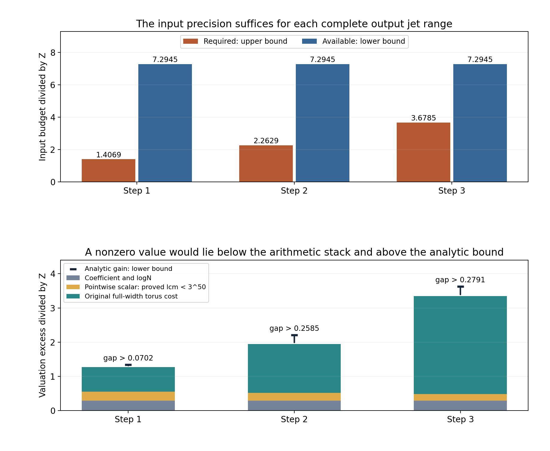
Figure 10.19. The constants, floors and permitted coefficient family are those of (10.245), with \(k=50,L=35299\) and the proved clearing bound \(3^{50}\). Each upper panel pair compares the available lower input budget \((U+G_0)/Z\) with the required upper budget \((n_j\mu_j\theta+\mu_jM_0)/Z\). The lower stacks are certified upper bounds from the coefficient, individual scalar and full-width torus terms in (10.244); the black marks are the certified analytic lower bounds. Their strict gaps force zero values. These are bounds rather than sampled valuations of an auxiliary function. Lemma 10.91 proves actual normality, Theorem 10.92 proves the full pointwise budget, and Theorem 10.93 proves all three integer extensions. Solution 39 reconstructs every bound. Figure program. Human-source context: Yu's free paper, Lemma 5.2 and equations (5.25)–(5.38).
32. Nested integer jets and the first fractional step
Earlier integer extensions retain more derivatives at their inner nodes. These derivatives can be used together. The following interpolation argument keeps the full nested distribution rather than assigning its smallest multiplicity to every node.
Hermite interpolation on nested intervals
Lemma 10.94 (nested normal-series interpolation). Let \(0\le R_0<\cdots<R_m\) be integers and let \(\mu_0\ge\cdots\ge\mu_m\ge1\) be integers. Put
\[ \begin{aligned} E_j&=[-R_j,R_j]\cap\mathbb Z,& \mu(s)&=\mu_j\quad(s\in E_j\setminus E_{j-1}),\\ E_{-1}&=\varnothing,& N_*&=(2R_0+1)\mu_0+ 2\sum_{j=1}^m(R_j-R_{j-1})\mu_j . \end{aligned} \tag{10.247} \]Choose \(v_p(\rho)=\theta>0\), a normal series \(F\), and \(C\ge0\). Set \(B=\lfloor\log_p(2R_m)\rfloor\) when \(R_m\ge1\), and \(B=0\) when \(R_m=0\). Suppose \(v_p(F_h(\rho s))+h\theta\ge\Lambda-hC\) for \(s\in E_m\) and \(0\le h<\mu(s)\). Then
\[ v_p(F(\rho x))\ge \min\{N_*\theta,\ \Lambda-(\mu_0-1)\max\{B,C\}\} \qquad(x\in\mathbb Z_p\subset\mathbb Q_p). \tag{10.248} \]Proof. For \(s\in E_m\), form the rational polynomial \[ L_s(X)=\prod_{\substack{t\in E_m\\t\ne s}} \left(\frac{X-t}{s-t}\right)^{\mu(t)}. \] It has value one at \(s\) and a zero of order \(\mu(t)\) at every other node \(t\). We claim \[ v_p(L_s(x))\ge-(\mu_0-\mu(s))B\qquad(x\in\mathbb Z_p). \] The claim holds at a node by its zero or unit value, so consider a point that is not a node. Decompose the exponents as \[ \mu(t)=\mu_m+\sum_{j=0}^{m-1}(\mu_j-\mu_{j+1})\mathbf1_{t\in E_j}. \] For a full integer interval, the counts in residue classes modulo \(p^a\) differ by at most one. If \(s\in E_j\), the contribution of that interval, omitting \(s\), at level \(a\) is \[ N_a(x)-N_a(s)+1-\mathbf1_{x\equiv s\pmod{p^a}}\ge0. \] If \(s\notin E_j\), no node is omitted and the contribution is \(N_a(x)-N_a(s)\ge-1\). For \(a>B\), every denominator difference \(s-t\) has valuation less than \(a\), since \(0<|s-t|\le2R_m<p^a\); those remaining contributions are nonnegative. The base interval \(E_m\) always contains \(s\). Only increments belonging to intervals not containing \(s\) can lose valuation, and their sum is \(\mu_0-\mu(s)\). This proves the claim.
The formal Taylor inverse \[ A_s(U)=L_s(s+U)^{-1} =\prod_{t\ne s}(1+U/(s-t))^{-\mu(t)} \] has its degree-\(h\) coefficient of valuation at least \(-hB\). Each factor has integer binomial coefficients, and each denominator difference has valuation at most \(B\). Consequently the Hermite polynomial is \[ H(\rho X)=\sum_{s\in E_m}L_s(X) \sum_{h=0}^{\mu(s)-1}\rho^h F_h(\rho s)(X-s)^h [A_s(X-s)]_{\le\mu(s)-1-h}. \] Its degree is at most \(N_*-1\), and its divided jets at each node agree with those of \(F\) through order \(\mu(s)-1\). A summand with inverse coefficient of degree \(a\le\mu(s)-1-h\) has valuation at least \[ \Lambda-(\mu_0-\mu(s))B-hC-aB \ge\Lambda-(\mu_0-1)\max\{B,C\}. \]
For completeness, the normal quotient argument of Lemma 10.33 applies to the nonuniform root polynomial \(W(Z)=\prod_s(Z-\rho s)^{\mu(s)}\). Indeed \(W=Z^{N_*}-A\), where every coefficient of \(A\) has positive valuation. Write \(Q\) and \(R\) for quotient and remainder on division by \(Z^{N_*}\). Both have Gauss operator norm at most one. Let \(M_A\) mean multiplication by \(A\). The convergent series \[ G=\sum_{j\ge0}(Q\circ M_A)^jQF \] is normal, because multiplication by \(A\) strictly decreases Gauss norm and the normal-series algebra is complete by Lemma 9.2. With \(H_0=R(F+AG)\), one has \(F=H_0+WG\), \(\deg H_0<N_*\), and \(H_0\) is normal. Its jets are the required jets. Uniqueness of the polynomial with those jets follows because a polynomial of degree less than \(N_*\) divisible by every \((Z-\rho s)^{\mu(s)}\) is zero. Thus \(H_0=H\).
Finally \(v_p(W(\rho x))\ge N_*\theta\), and \(G(\rho x)\) is integral. Combining this with the bound on \(H\) proves (10.248). \(\square\)
In the prepared-family setting, suppose the values at a node in the \(j\)-th interval are zero through total order \(T_j\). For a desired output order \(T'\), choose nonincreasing multiplicities \(\mu_j\le T_j-T'+1\). Lemma 10.38 and the common normality scale of Proposition 10.37 give the hypotheses of Lemma 10.94 with \(\Lambda=U-\beta+G_0\) and \(C=C_0\). If \(M_0=\max\{B,C_0\}\), then \(\beta\le M_0\), so the sufficient input inequality is
\[ U+G_0\ge N_*\theta+\mu_0M_0. \tag{10.249} \]Under this inequality the prepared analytic valuation excess is at least \(N_*\theta-G_0\) at every \(x\in\mathbb Z_p\), for every total prepared order at most \(T'\). The comparison with the unprojected family uses the same projection estimate as Corollary 10.40; no new precision hypothesis is introduced.
The original first fractional range
Theorem 10.95 (the first fractional step for the rational family). Under the hypotheses and with the initial family of Theorem 10.93, put \(S_1=\eta^{-3}S\), \(T_1^*=\eta^3T\). Then
\[ \Phi_0(s/2;\boldsymbol t)=0 \quad\text{for }\ |s|\le2(\lfloor S_1\rfloor+1)=1374,\qquad |\boldsymbol t|\le\lfloor T_1^*\rfloor=993090. \tag{10.250} \]This range uses the original unfloored \(S,T\), and the coefficient family is the whole family (10.245).
Proof. Theorem 10.93 and the initial construction give these nested integer data.
| \(j\) | Radius \(R_j\) | Available order \(T_j\) |
|---|---|---|
| 0 | 379 | 1796752 |
| 1 | 758 | 1474535 |
| 2 | 1517 | 1210101 |
| 3 | 3034 | 993090 |
For output order \(T'=993090\), take \[ (\mu_0,\mu_1,\mu_2,\mu_3)=(780000,481446,217012,1). \] Each multiplicity is at most the available order minus \(T'\) plus one. The ring counts are \(759,758,1518,3034\), hence \(N_*=1286383318\). Here \(B=7\), \(C_0\le46\), and \(M_0=46\). The certified bounds are \[ \frac{N_*\theta+780000\cdot46}{Z}\le7.244899709935 <7.294535093395\le\frac{U+G_0}{Z}. \] Thus (10.249) holds. The analytic valuation excess at every fractional output argument, divided by \(Z\), is at least \(7.100020502185\). Division by two preserves membership in \(\mathbb Z_3\).
We must retain the field of these values. Put \(\gamma_1=-8,\gamma_2=-125\) and \(\eta_i=\exp(\tfrac12\log\gamma_i)\). Their logarithms have valuation two, so Lesson 9 proves that these are square roots in \(\mathbb Q_3\), each congruent to one. Their global field is \[ F=\mathbb Q(\eta_1,\eta_2) =\mathbb Q(\sqrt{-2},\sqrt{-5}),\qquad [F:\mathbb Q]=4. \] The two square classes are independent: \(-2,-5,10\) are all nonsquares, as their prime valuations or signs show. Equivalently, if \(\sqrt{-5}=a+b\sqrt{-2}\) with rational \(a,b\), squaring forces \(ab=0\); \(b=0\) would make \(-5\) a rational square, and \(a=0\) would make \(5/2\) a rational square. Both are impossible. This proves the degree. The chosen completion of \(F\) is \(\mathbb Q_3\), since \(F\subset\mathbb Q_3\) and \(\mathbb Q\) is dense there. Hence its chosen \(e,f\) are one. Every normalized monomial at \(s/2\) is a product of integer powers of \(\eta_1^s,\eta_2^s\), so every prepared value belongs to this ambient field. Individual values may belong to a proper subfield; the bound over \(F\) remains valid.
The outward parameter intervals give \[ 686.229279178168\le S_1\le686.229279178169. \] Thus \(X=687\) covers the entire output range. In Theorem 10.92 take \(I=0,J=1,R=X+99=786\), the same common Euler bound of Theorem 10.93, and \(T'=993090\). Its scalar maximum, using the proved upper clearing bound \(3^{50}\), occurs at additive order \(470396\), leaving Euler order \(522694\). The ratio tests are exact integer products. The entropy estimates proved in Solution 39, with the negative factorial logarithm retained, give \(\ln\mathcal H_0^{\rm fine}/Z\le0.208379911543\).
Also \(v_2(50!)=25+12+6+3+1=47\). Equation (10.243) therefore gives the common denominator exponent \[ \Xi_{0,1,u}\le D_{\mathrm a}+47L=3424003 \] for every additive order. This deliberately retains a valid common upper bound; the order recovery can only improve it.
The four terms inside the arithmetic bracket of (10.244), divided by \(Z\), have the following certified upper bounds.
| Term | Upper bound |
|---|---|
| Coefficient height and \(\tfrac12\ln N\) | 0.310842088027 |
| Individual scalar logarithm | 0.208379911543 |
| q-denominator logarithm | 0.008748404912 |
| Original full-width torus height | 0.714102914710 |
Multiplying their sum by the actual ambient global-to-local factor \(4/\ln3\), using the unrounded rational intervals before the final rounding, gives an arithmetic valuation excess at most \(4.522335429896Z\). It is strictly smaller than the analytic lower bound. Their gap exceeds \(2.577685072290Z\). Thus every nonzero prepared value would contradict (10.244); orders above \(D_{\mathrm a}\) are already zero. This proves (10.250). \(\square\)
This completes the first fractional step for the stated original rank-two family. The q-coset extraction, subsequent contracted families, other parameter cases, stopping branches and final multiplicity argument remain separate mathematical requirements.
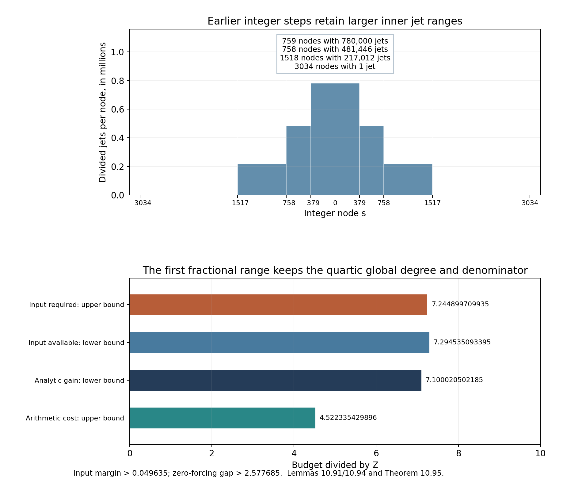
Figure 10.20. Each unit cell in the upper panel represents one integer node, with constant height equal to its available multiplicity \(\mu(s)\); cell edges are half-integers. The exact interval radii are \(379,758,1517,3034\), and the four ring counts and multiplicities give \(N_*=1286383318\). The lower panel shows certified bounds divided by \(Z\): the input required is below the input available, and the arithmetic upper bound is below the analytic lower bound. The arithmetic cost includes the quartic ambient field and the full common q-denominator exponent \(3424003\). These are proved bounds, not sampled values of an auxiliary function. Lemma 10.94 proves the nested interpolation; Theorem 10.95 proves the exact original first fractional range; Solution 40 checks the Hermite basis and calculations. Figure program. Human-source context: Yu's free paper, Lemma 5.3.
33. Exercises with solutions
-
Easy. Explain exactly how nonunit bases can be reduced to unit bases. Give an example showing that the conclusion of Theorem 10.8 cannot be extended unchanged to nonunits.
-
Medium. Derive (10.34) from (10.22), including the maximum in \(H\).
-
Medium. Prove (10.36) using the residue order and the power laws. Explain where the assumption that \(p\) is odd enters.
-
Medium. For \(K=3,L=4,p=3,e=1,t=0,u=0\), find the lower bound supplied by (10.10). Find the valuation precision required in its hypothesis, and the exact excess in the row expansion when \(n\) ordinary rows are used.
-
Easy. Show that (10.6) is attained for \(K=2,L=4,R=3\). Identify the maximizing list of first coordinates.
-
Medium. A proposed assertion for every prime \(p\) and pair of coprime positive integers \(x,y\) bounds \(v_p(x^{p-1}-1)\) by \(283(p-1)\ln y\ln(xy)/(\ln p)^2+4\). Show why it is false as stated when \(y=1\), without using a logarithm estimate.
-
Hard. Adapt the determinant argument to the hypotheses of Theorem 10.11. Explain why its first-base precision, unit coefficient after removing the common p-part, and second-base condition at two are all recorded. Derive the power \(E^{-3}\) in its final bound.
-
Medium. Compute \(M_2(4,9)\) over \(\mathbb Q\), prove (10.48) in this example, and compute the residue index (10.49) at five.
-
Hard. Derive the constant 58 in (10.55) directly from (10.53), including the roles of the chosen height radius and the selected archimedean weight. For the rational bases 4,9, compute the full saturation index, its root-of-unity factor, and the diamond average in Figure 10.2.
-
Medium. Apply Theorem 10.21 to the rational unit 2 at three. Determine its residue order and exact valuation for every nonzero exponent with a nonzero power difference. Compare the bound with the normalization in a field of degree two having local degrees e=1, f=2.
-
Medium. At p=5 take \(L_1=5z_1+z_3\), \(L_2=5z_2+z_3\), \(L_3=-5z_1-5z_2-z_3+z_4\), and \(L=L_1+L_2+L_3=z_3+z_4\). Compute the matrix in Lemma 10.23 and all its two-column upper minors. Choose a minimum-valuation derivative basis. Explain the denominator introduced by the other natural basis.
-
Hard. Set \(r=2,S=T=90\), \(D_0=32,D_1=2,D_2=3\), and \(S_i=T_i=30\). Show that Theorem 10.25 implies that a polynomial of these bounds with all the stated jets zero at \((s,2^s,3^s)\), \(0\le s\le90\), is zero, for every nonzero rational vector \(\boldsymbol B\). Check the integer degree inequalities and both possible one-dimensional relation bounds.
-
Medium. In Theorem 10.27 take \(K=\mathbb Q,p=5,n=2\), bases \(2,3\), coefficients \(1,1\), and \(L_1=z_1+z_2\). Use \(\sigma=\ln6,H=10\ln5\). Compute the original saturated residue index, \(w_q,R_2,M_\gamma\), and verify the one-base height-product hypothesis without a numerical approximation. What valuation is being bounded?
-
Hard. For \(k=L=2\), compute the four shifted-power polynomials in Figure 10.4 and the determinant of their coefficients of \(X,X^2,X^3,X^4\). For \(k=\ell=2\), evaluate \(v(k)^m\Theta(1/3;k,\ell,m)\), \(0\le m\le4\), and check the exact q-power clearing bound with \(q=3,I=1\).
-
Medium. Use Theorem 10.32 over \(K=\mathbb Q\) with \(r=2,k=L=1,S=T=0\), \(\vartheta=(2,3)\), \(A_1=A_2=1\), \(D_1=Y_1\partial_{Y_1}-Y_2\partial_{Y_2}\), and exponents \((0,0),(1,0),(0,1)\). Compute \(N,M,\mathcal B\), exhibit a nonzero integral coefficient vector, and compare its exact projective height with (10.96). Form the ordinary polynomial \(P\) and identify which jets are imposed.
-
Hard. For the full node set with \(p=3,R=3,\mu=2,\theta=1\), what precision in (10.100) suffices for conclusion \(v_3(F(\rho x))\ge14\)? For \(p=2,q=3,R=3\), compute \(L_{-2}(0)\) in the q-deleted set and its valuation. Finally, why is the restriction \(x\in\mathbb Z_p\subset\mathbb Q_p\) essential to the full-set cardinal bound? Use \(p=2,R=1\) and an algebraic \(x\) with \(x^2=2\).
-
Medium. In Proposition 10.37 take \(p=3,q=2,I=0,k=L=2,\rho=3\), and a single nonzero coefficient \(c=1\) at \(\boldsymbol m=0,a=0,\ell=2\). At prepared index zero, compute \(\gamma,\Gamma\), and the polynomial \(F(Z)\). Check (10.107) for \(s=0,j=1\). If a torus factor with slope \(w\) is added, compare the sufficient slope hypothesis for \(w=9\) and \(w=3\).
-
Hard. At two, take the additive prepared polynomial \(f(y)=\Delta(y;2)=(y+1)(y+2)/2\), with \(I=0,k=2,L=1\) and no torus dependence. Show that its prepared values through order two at zero are integral, whereas its first ordinary divided jet has valuation \(-1\). Explain the exact role of \(C_0\). Next take full interpolation nodes with \(p=3,R=3,\mu=2,\theta=1\), and weighted jet precision \(\Lambda-jC\) with \(\Lambda=16,C=2\). Compare Theorems 10.34 and 10.39.
-
Medium. At \(p=3\), take \(q=2,k=L=1,I=0,J=1,c=1\), no torus dependence, and \(x=1/2\). Compute the prepared value \(\Delta(x;1)\), the clearing exponent in (10.115), and the bound (10.116) with \(X=1/2,T=0\). Distinguish the denominator cost at two from the valuation at three.
-
Hard. Let \(K=\mathbb Q,p=3,q=2,J=1,\vartheta=10\). Use the exponential and logarithm to choose a square root \(\eta\in\mathbb Q_3\) congruent to one. Determine the coefficient (10.117) for \(F=\mathbb Q(\eta)\). At \(s=1,x=1/2\), with \(k=L=1,I=0\), take exponents \(1,3\) and coefficients \(1,-1\). Factor the prepared value into its common local unit and a rational value, and compute its valuation. Compare the bounds from the root field and the common-factor rule, with \(X=1/2,T=0\).
-
Medium. Use \(I=0,k=2,L=1,X=2,r=2,\Omega_1=1,T=2\). Compute \(\mathcal P_{0,2}(Z)\), \(\mathcal B_0^*(2,2)\), and the earlier \(\mathcal B_0(2,2)\). At \(x=2,a=1,\ell=1,\omega_1=1\), show that the three additive bounds are attained.
-
Hard. In Corollary 10.45, take \(K=\mathbb Q,r=1,k=2,L=1,S=2,T=0\), \(\vartheta=2\), and \(\mathcal M=\{0,1,2\}\), so \(A=2\). Compute the separate-row bound (10.127) and the uniform averaged bound (10.128). Order the six columns by \((m,a)=(0,0),(0,1),(1,0),(1,1),(2,0),(2,1)\). Verify that \((2,-18,-57,36,1,0)\) is an integral kernel vector at all five nodes, and compute its two projective heights. Explain why the zero row at \(s=-2\) does not invalidate either bound.
-
Medium. In Theorem 10.47, take \(q=2,r=1,F=\mathbb Q,\vartheta=2,\eta=\sqrt2\). Show that at \(s=2\), the coefficients \(A_0=-2,A_1=1\) give a zero total sum whose separate coset coefficients are nonzero. Give a similar example with odd \(s\) in which the full-degree hypothesis fails. Finally, at \(p=7\), use the local square root \(\eta\equiv3\pmod7\) of two to show that finite valuation precision of a total sum need not transfer to its cosets.
-
Hard. Let \(q=2,p=3,r=2\), use one Euler argument \(\omega(\boldsymbol m)=m_1\), and retain \(m\equiv1\pmod2\), with \(m_*=1\). Compute the affine binomial change \(\Delta(2Z+1;t)\) through order two and its inverse. Verify the minimum-valuation identity on the new jet vector \((1,3,9)\). Explain why it preserves total order when combined with an unchanged additive index. Then apply Corollary 10.49 over \(K=\mathbb Q\) with \(\alpha_0=-1,\theta_1=2,\theta_2=3,P=3,d_1=1,d_2=0\): identify \(F\), the two phased roots and bases, their heights, and the root degree over \(F\).
-
Hard. Use the divided support in Figure 10.8. Compute \(a_0,H\), both subclasses and their phase factors after multiplication by \(\zeta^s\). If a coefficient of minimum valuation belongs to \(\lambda_0=(-1,0)\), state the retained phase congruence and normalized root-of-unity factor. Explain why the subclass is chosen independently of \(s\) and the derivative index. Compare the coprime case \(q=2,G_0=5,a_*=2\).
-
Hard. Over \(\mathbb Q_5\), apply the Newton construction to \(f(X)=X^2+1\), starting at \(x_0=2\). Compute \(x_1,x_2\), the three error valuations and the primitive fourth root \(\zeta\) modulo \(625\). Take \(K=\mathbb Q,\alpha_0=-1,q=2,\theta_1=2\), and \(g=2/\zeta\). Prove \(v_5(g-1)=1\). For the target \(\vartheta=3\), verify the choices \(t=0,j=3,P=125,d_1=-125\) in Lemma 10.53 and compute the exact valuation of \(\gamma_1-1\).
-
Medium. In Corollary 10.54, assume the other hypotheses and \(\mathcal A_{\mathrm{ph}}(4,4)=11\). Take \(p=3,q=2,R=4,T=5,\mu=2,k=L=2,\theta=3,C_0=0\). Compute the exact input node set, \(n,B,M_0,T'\), and the least \(U\) meeting the exact first budget. State the resulting zeros. Compare both lines of the alternative larger-scale budget; explain why its first line alone does not give the same zero conclusion.
-
Hard. In Figure 10.9, verify that the individual \(\gamma_i\) lie outside \(\mathbb Q\), whereas every normalized row entry is rational. Determine \(N,M_*,H_{\mathrm{ph}}\), and check the vector \((-b,C,-C,b)\) at all three nodes. Factor its torus polynomial, compute its two projective heights and its minimum 5-adic coefficient valuation, and compare its height with (10.152). Explain why the zero first row does not invalidate the bound.
-
Hard. Use the data of Figure 10.10. Compute the cancelled congruence and \(h_\Lambda\), prove the degrees and chosen completions of \(E\) and \(F\), and evaluate both 5-adic valuations of \(V\). For \(I=0,k=L=1,\lambda_0=0,c=(1,-1),s=1,x=1/2,\boldsymbol t=0\), compute every term in (10.156). Compare the support-field budget with the budget from the full root field, and explain why equal local degrees do not justify using the original global degree.
-
Medium. Verify the auxiliary-prime choices in Corollary 10.9 for \((a,p)=(8,3),(3,2),(25,2)\). Compute the exact original and transformed valuations, the rational heights and the cutoff \(H\). Derive the all-power bound when \(b=1\), retaining the same \(250000\ln(5a)\ln5\) coefficient. Explain why simply setting the second base to one would not prove this case.
-
Hard. Verify the two support heights in Figure 10.11 by clearing denominators in the monomial vectors and finding their primitive integer coordinates. Compute both signed heights of \(\{(0,0),(1,0),(0,1)\}\). Extract the even-even coset from the diamond at \(q=2\), use reference \((-2,0)\), and verify (10.162). At \(P=1,S=1,k=L=1,T=0\), compare the separate-row coefficient budgets for the seven-point diamond support using its exact height and its coordinate box. Explain how a shifted original-coordinate box is handled when its centre is outside the image of \(B\).
-
Hard. Verify the two initial kernels in Figure 10.12 and determine their exact row fields. Prove the discriminants \(5\) and \(24\) using the full integral bases of the two quadratic fields. Compute both projective coefficient heights, explain why their finite-place contributions vanish, and evaluate (10.171) with the actual row-field discriminant for each example. For \(t=\sqrt6\), compare the one-generator discriminant bound with the bound using only the maximum support height. Explain what happens to the row field when \(S=0\), and why \(N>M_*\) and the later analytic inequalities still need checking.
-
Medium. Verify every lattice and phase coordinate in Figure 10.13. Compute \(J,V/\Delta,g,H\), the guaranteed class size, and both sides of (10.180) at \(k=2,L=1\). At \(S=1,T=0\), compare the coefficient surplus certified by the exact class count with the coarser volume criterion. Then take \(T=1\) and one nonzero Euler direction: compute \(M_*\), and state precisely what the counting criterion does and does not prove. Explain why replacing the closed box by an open one would invalidate the integer-volume argument.
-
Hard. Use \(K=\mathbb Q,p=3,r=2\), \((\alpha_1,\alpha_2)=(2,5)\), and \(c_0=1.9,c_1=1.4494,c_3=1.3852,c_4=20.8\). Put \(a_0=2+\ln14\), \(a_1=4.79\), \(g_0=3(2a_0+a_1+\ln(2a_0+a_1))\), \(h=g_0\), and \(\tau=1/(4\cdot10^{26})\). Use \(\widehat\vartheta=3/2\) and \(\sigma_1=\ln2,\sigma_2=\ln5\). Prove that \(J=1,u=1,H=1\). Verify the floors in Figure 10.14 with rigorous bounds, construct a support of exactly \(\lfloor D_1D_2\rfloor+1\) points without listing it, and compute \(N,M_{\rm full},M_*\). Use the integral identity \(20N-57M_{\rm full}>0\) to verify the strict surplus. Identify the actual coefficient field and its discriminant cost.
-
Hard. First take \(K=\mathbb Q(\zeta_3,\sqrt2)\) and \(p=2\). Prove that \(d=4,e=2,f=2,u=1\), and verify equality in (10.192). Then return to all the rational parameters of Solution 34. Compute \(\Omega_1\), the actual clearing integer, both maximizing additive orders in (10.199) and (10.201), and the exact mean orders in (10.204). Reconstruct each signed component and net height bound in Figure 10.15, using (10.174) with the actual ratio \(M_* /(N-M_*)\). Include the row-scaling bounds of Corollary 10.80. Explain why the coefficient field and all zeros are preserved by the alternative global clearing.
-
Medium. Reconstruct every exact lower-bound path and final depth in Figure 10.16. Distinguish these lower bounds from the actual valuation path for \(\beta=1+\sqrt2\) in \(\mathbb Q_2(\sqrt2)\). Next let \(\pi^3=3\), \(L=\mathbb Q_3(\pi)\), and \(\beta=1+\pi\). Show that the bound (10.210) is attained at \(P=9\), and use the exponential coefficients to prove that the closed boundary radius \(3^{\vartheta}\) cannot replace \(3^\theta\) in Corollary 10.82. Describe the coherent principal square root of the phased coordinate for \(\alpha=-\beta,\zeta=-1\).
-
Hard. Reconstruct Figure 10.17 over \(K=\mathbb Q\) at \(p=5\). Prove that the q-primary saturation lattice of \(4,9\) has basis \(B=\tfrac12I\) and index \(J=4\), and identify the even phase class of its generators \(2,3\). Compute the exact prepared Euler range at reference \(0\), and again at reference \((8,0)\). Explain why the full box widths give a bound without a factor two, and why omitting \(J\) can even destroy integrality. Then return to Solution 34 and use (10.222)–(10.228) to certify the uniform initial height bound, retaining every field and scalar cost.
-
Hard. Reconstruct Figure 10.18 for \(K=\mathbb Q(\sqrt5)\), with original bases \(5,7\) and coefficients \(b_1=b_2=1\). Determine the full saturation lattice and its q-primary index at \(q=2\), verify \(B'=BU\), and compute both lists of generator heights. Identify the field and its discriminant. At \(p=3\), determine \(e,f,u,\nu,P\) and the phase classes. Use the constants of Solution 34, put \(g_0=3(2a_0+a_1+\ln(2a_0+a_1)+\ln2)\), \(h=g_0\), \(\sigma_1=\ln5,\sigma_2=\ln7\), and retain its \(\tau\). Certify the original \(g_{11},g_{12}\), a strict initial column surplus, and the full bound (10.235). Compare the generator field with the smallest field of the actual rows.
-
Hard. Reconstruct Figure 10.19 for the entire coefficient family (10.245). Obtain a rigorous common Euler-argument bound and a bound for \(v_3(b_2)\), then determine every \(R_j,T_j,\mu_j,n_j,B_j\). Certify both comparisons at all three integer steps, retaining the complete pointwise factorial and lcm costs. Explain how a ratio search bounds the enormous Euler binomial without constructing it, and why these integer comparisons do not establish the fractional descent.
-
Hard. Derive the five Hermite basis polynomials for \(R_0=0,R_1=1,\mu_0=3,\mu_1=1\), checking every divided jet. Reconstruct the nested weights, total multiplicity and both strict comparisons in Theorem 10.95. Explain why equality of the chosen completions does not remove the quartic arithmetic factor, and why evaluating the denominator cost only at the scalar-maximizing order need not bound the joint maximum.
Solution 1. Put \(q_i=v(\alpha_i)\). If \(b_1q_1\ne b_2q_2\), the ultrametric inequality gives the exact valuation \(\min(b_1q_1,b_2q_2)\), so no cancellation estimate is needed. If they are equal, choose \(\pi=p^{1/e}\) in an algebraic extension and set \(\epsilon_i=\alpha_i\pi^{-e q_i}\). The exponents \(e q_i\) are integers, the \(\epsilon_i\) are units, and
\[ \alpha_1^{b_1}-\alpha_2^{b_2} =\pi^{e b_1q_1}(\epsilon_1^{b_1}-\epsilon_2^{b_2}). \]The valuation is \(b_1q_1\) plus the unit-difference valuation. The field degree, heights, and any dependence of the new bases must be checked anew. The linear offset cannot be discarded. For instance, \(3\) and \(6\) are multiplicatively independent but nonunits at three, and \(v_3(3^m-6^m)=m+v_3(1-2^m)\ge m\). A bound by a fixed multiple of \((1+\ln m)^2\) cannot hold. Thus unit normalization reduces the cancellation problem; it does not preserve the unadjusted bound.
Solution 2. Use rational heights \(h(a)=\ln a\), \(h(b)=\ln b\), and the choices \(\ln A_1=\ln(5a)\), \(\ln A_2=\ln(5b)\). Coprimality makes both exponents vanish in a multiplicative relation. Also
\[ \ln B'+\ln\ln p \le\ln(p-1)+\ln(2/\ln5)+\ln\ln p \le3\ln p. \]Hence the maximum is \(10\ln p\), not the smaller first term. Squaring it cancels two of the four denominator powers of \(\ln p\); \(2500\cdot100=250000\). This proves (10.34).
Solution 3. The residue field group has order \(p-1\), so the order \(q\) of \(a/b\) divides it. A nonmultiple of \(q\) gives valuation zero. For \(n=qm\), prime-to-p powers preserve the valuation of \((a/b)^q-1\), and each p-th power adds one because its initial valuation is an integer at least one. For odd \(p\), one is strictly greater than \(1/(p-1)\), so the boundary case does not occur. The same calculation for \(p-1=q((p-1)/q)\) has no p-part. Combine the two identities and Corollary 10.9. At \(p=2\), valuation one lies on the boundary; for example \(v_2(3^2-1)=3\), whereas \(v_2(3-1)+v_2(2)=2\).
Solution 4. Here \(N=12\), \(c_0=1\), and \(\sum_i k_i=12\). Formula (10.10) gives
\[ v_3(\Delta)\ge54-\frac{12\ln12}{\ln3}. \]Its hypothesis is \(v_3(\Lambda)\ge23/2\), equivalently at least twelve when the difference lies in \(\mathbb Q_3\). Before the common logarithmic loss, the contribution from \(n\) ordinary rows is at least
\[ (12-n)\frac{23}{2}+\frac{n(n-1)}2-12 =54+\frac{(12-n)^2}2. \]Thus its excess over the common minimum is exactly \((12-n)^2/2\). This is a lower bound for a summand's valuation, rather than an equality for that valuation.
Solution 5. Order the row labels as \(0,0,1,1,2,2,3,3\), and take \(r_i=0,0,0,0,2,2,2,2\). Then \(\sum_i r_i=8\), \(\sum_i l_ir_i=20\), and the center is \(12\). The error is eight, equal to \(NL(R-1)/8=8\). Reversing the chosen zero and two coordinates attains the negative error.
Solution 6. Take \(p=3\), \(x=3^{10}+1\), \(y=1\). The pair is coprime and \(p\nmid x\). Factor \(x^2-1=(x-1)(x+1)\). Its valuation is ten, because \(x-1=3^{10}\) and \(x+1\equiv2\pmod3\). The proposed right side is four, since \(\ln y=0\). This disproves the unrestricted statement. All the estimates used above have their hypotheses proved and stated separately.
Solution 7. Remove residue roots in the selected congruence class, and remove the common p-part of the coefficients by the deep-unit power law. The chosen base has \(v(\log\epsilon_1)\ge E\). The assumption \(p\nmid b_2'\) gives integral nodes \(r+(b_1'/b_2')s\); it cannot be dropped from this construction when the first base alone supplies \(E\). The second principal unit must already lie in the exponential domain because the exponent multiplier is now one. At odd primes its positive integer valuation does this automatically; at two the additional depth condition supplies it.
The pure minor of order \(n\) has the bound in the proof of (10.40), while complementary error rows cost at most \(E\sum k_i\). A difference precision \(E(N-1/2)\) and the identity (10.14) give \(ENK(L-1)/2-N\ln N/\ln p\). Compare this with the same centered polynomial height bound, now without any exponent multiplier. Use \(a_i=\ln A_i/(E\ln p)\), \(B=H_E/(E\ln p)\), and \(G=p-1\). The cardinalities and inequalities are exactly those checked in (10.40)–(10.42); the collision branch uses the residue order before applying \(X-1\) Liouville. The final budget is
\[ EzB^2 =E(p-1)\frac{\ln A_1\ln A_2}{E^2(\ln p)^2} \frac{H_E^2}{E^2(\ln p)^2} =\frac{p-1}{E^3(\ln p)^4}\ln A_1\ln A_2H_E^2. \]This accounts for every power of \(E\); replacing the established coefficient \(1300\) by \(88000\) gives the asserted weaker version.
Solution 8. If a rational \(\beta\) realizes \(\boldsymbol v\) in (10.44), valuation at two gives \(v_2(\beta)=2v_1\), and valuation at three gives \(v_3(\beta)=2v_2\). Hence both coordinates lie in \(\tfrac12\mathbb Z\). Conversely every such vector is realized by \(\beta=2^{2v_1}3^{2v_2}\), with a common denominator \(T\) in (10.44). Thus the stated saturated lattice and the bases \(2,3\) are exact. If \((-1)^{a_0}2^{a_1}3^{a_2}\) is a rational square, prime valuations make \(a_1,a_2\) even, and positivity makes \(a_0\) even. The three square classes are independent, so the proved Kummer degree lemma gives degree eight. At five, the residue of two has order four, since \(2^2\equiv-1\pmod5\). The residue group generated by \(-1,2,3\) is therefore the whole group of order four. Its index is one.
Solution 9. The choice \(H=\exp(n/(2d))\) cancels the \(2^n\) in the diamond volume and the \(H^{2d}=\mathrm e^n\) in the count. The mixed complex term contributes the additional factor \(\mathrm e^{-n/2}\le1/\sqrt{\mathrm e}<2/3\). Its two coefficients in (10.53) are less than 31 and 32, so their total is less than \(31(2/3)+32=158/3<58\). The real coefficient is less than 33. The selected archimedean weight is \(f\ell/d\); only \(\ell(d-f)/d\) remains for the other archimedean Hadamard factors. This exact division gives (10.50), before any numerical constant is chosen.
For rational 4,9, the valuations at two and three in (10.54) force \(2v_1,2v_2\) to be integers, for any realizing integer \(T\). Conversely \(\beta=2^{2v_1}3^{2v_2}\) realizes every half-integral vector. Hence \(M_{\mathbb Q}=\tfrac12\mathbb Z^2\), its index is four, and \(w_{\mathbb Q}=2\), since the only rational roots of unity are \(1,-1\). Thus the left side of (10.55) is eight. For \(H=\mathrm e\), (10.56) gives \(V=2/(\ln4\ln9)\) and average \(4V=8/(\ln4\ln9)\). The three points \((-1/2,0),(0,0),(1/2,0)\) lie in the open diamond, while the other points of its zero lattice coset lie outside. Their values are \(1/2,1,2\), and the six signed values are distinct and have multiplicative height at most two, which is less than \(\mathrm e\).
Solution 10. The residue of 2 at three is -1, of order two. An odd exponent gives valuation zero. For even b, factor through 2^2=4; since v_3(4-1)=1, the proved power law gives \(v_3(2^b-1)=1+v_3(b)\), also for negative b by unit inversion. The height is \(\ln2\), so (10.59) with \(d=e=f=1\) gives \(v_3(2^b-1)\le v_3(b)+4\ln2/\ln3\). In a field with \(d=2,e=1,f=2\), the ratio \(d/f\) is still one, the residue of the rational unit is still -1, and \(\operatorname{ord}_{\mathfrak p}=v_3\). The same expression therefore follows. A degree-only bound that discarded f would be larger, and a normalization omitting e in a ramified field would instead be incorrect.
Solution 11. Here \(b=(0,0,1,1)\), \(B=(1,1,1)\), and \[ C=\begin{pmatrix}5&0&1\\0&5&1\\-5&-5&-2\end{pmatrix}. \] The upper minors for column pairs \((1,2),(1,3),(2,3)\) are \(25,5,-5\), with valuations \(2,1,1\). Choose columns \(1,3\). The derivations are \(\delta_1=5(E_1-E_3)\), \(\delta_2=5(E_2-E_3)\), \(\delta_3=E_1+E_2-2E_3\), and \(\delta_2=-\delta_1+5\delta_3\). Their coefficients are 5-adically integral. Choosing columns \(1,2\) would instead give \(\delta_3=(\delta_1+\delta_2)/5\). For example \(\delta_2^2=\delta_1^2-10\delta_1\delta_3+25\delta_3^2\), so the minimum-minor change preserves integrality for the second-order jets too. The rank and Cramer arguments prove the assertion at every order.
Solution 12. Both sums of allocations are \(90\), and \(D_0=T_2+2=32\) is largest. The \(m=0\) inequality is \(31^2=961>32\). The \(m=1\) inequality is \(31\binom{32}{2}=15376>2\cdot32\cdot3=192\). The last inequality is \(15376>6\cdot32\cdot2\cdot3=1152\). The bases \(2,3\) are independent by their prime valuations. If the polynomial were nonzero, the theorem would supply \(\nu=1\). Choose \(A_1=A_2=1\); then \(C_{2,1}=2\), and any nonzero integral relation vector has \(R_1\ge1\). Its first possible bound is \(31R_1\le6\), and its second is \(961R_1\le384\). Both contradict \(R_1\ge1\). Thus no nonzero polynomial can have the proposed jets.
Solution 13. Prime valuations show that the q-primary saturated lattice of \(2,3\) over \(\mathbb Q\) is \(\mathbb Z^2\): any realizing power forces both rational exponents to be integers. At five their residues, together with \(-1\), generate all four nonzero classes. Thus \(\delta(\boldsymbol\alpha)=1\), while \(w_q=2\), \(q=2\), \(e_{\mathfrak p}=f=d=1\). We have \(a=28/3\) and \(R_2=14\mathrm e(1+\varepsilon_2)\).
Here \(\gamma=6\) has residue order one, so \(\delta_\gamma=4\) and \(M_\gamma=\max\{5/(4(\ln5)^2),\mathrm e\}=\mathrm e\). Indeed \(\ln5>1\) since \(\mathrm e<3\), and \(\mathrm e>2\). Also \(M_2\ge\mathrm e^2/4\). Consequently \[ R_2\frac{M_2}{M_\gamma}\ln2\ln3 \ge\frac72\mathrm e^2(1+\varepsilon_2)\ln2\ln3>7. \] The last inequality uses \(\mathrm e>2\), \(\ln2>1/2\) from its integral, and \(\ln3>1\). On the other hand \(\sigma=\ln6<2\), because the first four exponential terms give \(\mathrm e>8/3\), hence \(\mathrm e^2>6\). This proves (10.77). The height of the rational number 6 is exactly \(\ln6\). The chosen \(H\) exceeds all three required lower bounds. The valuation is \(v_5(6-1)=1\). Taking \(c=1790\) matches the rational unramified case of the free preparation; Theorem 10.27 supplies its fully proved numerical bound.
Solution 14. Put \(F_0=(X^2+3X+2)/2\), \(F_1=(X^2+5X+6)/2\). The four polynomials are \(F_0,F_1,F_0^2,F_1^2\), and their coefficient matrix is \[ \begin{pmatrix}3/2&5/2&3&15\\1/2&1/2&13/4&37/4\\0&0&3/2&5/2\\0&0&1/4&1/4\end{pmatrix}. \] Its lower left block is zero; the diagonal block determinants are \(-1/2,-1/4\), giving \(1/8\). Thus the polynomials are independent, despite their common root \(-2\).
For the Taylor calculation, \(v(2)=2\). At \(z=1/3\), \(\Delta(z;2)=14/9\), \(\Delta'(z;2)=11/6\), and \(\Delta''(z;2)=1\). Expanding its square at that point gives the prepared coefficients \[ \left(\frac{196}{81},\frac{308}{27},\frac{59}{3},\frac{44}{3},4\right). \] The exponent in (10.87) is \(\ell(kI+v_3(k!))=2(2+0)=4\). Multiplication by \(3^4\) gives the integers \(196,924,1593,1188,324\), as required. There is no denominator at five, so this clearing factor has no cost in the 5-adic valuation.
Solution 15. Here \(v(1)=1\), \(N=3\), \(M=1\), \(\Omega=1\), and \(\mathcal B=2\). The only equation is \(c_0+c_1+c_2=0\) at \((X,Y_1,Y_2)=(0,1,1)\). Take \(c=(-1,1,0)\). Then \(h_\infty(c)=0\) and \(h_2(c)=\frac12\log2\); the finite maximum norms are one. Formula (10.96) is \(h_2(c)\le\frac34\log3+\frac12\log2\), which holds strictly. Since \(\boldsymbol d=(1,1)\), the ordinary polynomial is \(P=Y_1Y_2(X+1)(Y_1-1)\). It is nonzero and vanishes at \((0,1,1)\). Only the order-zero value is imposed: the \(D_1\)-derivative there equals one, so no first-order vanishing is asserted. Every nonzero coefficient is a local unit at every prime, so the optional normalization changes nothing.
Solution 16. In the first case \(n=7,B=1,\kappa=0\). Theorem 10.34 gives \(v_3(F(\rho x))\ge\min\{14,\Lambda-1\}\), so \(\Lambda\ge15\) suffices. The larger logarithmic cost in Corollary 10.35 is sufficient but is not needed in this example.
The q-deleted set is \(\{-2,-1,1,2\}\), and \[ L_{-2}(0)=\frac{(0+1)(0-1)(0-2)}{(-2+1)(-2-1)(-2-2)}=-\frac16. \] Its 2-adic valuation is \(-1\). Thus the deleted-node cardinal factors need not be integral, whereas the full-node factors are integral at every \(x\in\mathbb Z_p\). The bound \(-B=-2\) is valid here.
For the last case the full nodes are \(-1,0,1\), and \(L_1(X)=X(X+1)/2\). The equation \(x^2=2\) gives \(v_2(x)=1/2\); since \(v_2(x)>0\), the ultrametric inequality gives \(v_2(x+1)=0\). Therefore \(v_2(L_1(x))=-1/2\), although \(x\) is integral in its extension. It lies outside \(\mathbb Q_2\), whose nonzero valuations are integers. The residue-count proof of Theorem 10.34 applies to \(\mathbb Z_p\), and does not assert this cardinal integrality on the entire integral ball of \(\mathbb C_p\).
Solution 17. Here \(D=4,\delta=0\), \(\gamma=3^4(2!)^2=324\), and \(\Gamma=4\). The unscaled polynomial is \(f(y)=((y+1)(y+2)/2)^2\), so \[ F(Z)=(Z+3)^2(Z+6)^2=Z^4+18Z^3+117Z^2+324Z+324. \] Its coefficients are 3-adically integral and its finite tail is zero, so it is normal. We have \(f_1(0)=3\) and \(F_1(0)=324\). Thus \(v_3(F_1(0))+1=5=\Gamma+v_3(f_1(0))\). The sufficient slope threshold is \(\theta+1/(p-1)=3/2\). It holds for \(w=9\), whose valuation is two, and fails for \(w=3\), whose valuation is one. Under scaling, the corresponding exponential is \(\exp(wZ/3)\); only the former meets the stated normal-series hypothesis.
Solution 18. Here \(v(2)=2\), and the prepared values at zero are \[ f(0)=1,\qquad v(2)f_1(0)=2\cdot\frac32=3, \qquad v(2)^2f_2(0)=4\cdot\frac12=2. \] Their 2-adic valuations are \(0,0,1\). Take \(P_0=0\) and \(\beta=0\); the additive part of Lemma 10.38 has \(C_0=v_2(v(2))=1\). It gives \(v_2(f_1(0))\ge-1\), with equality. Prepared integrality does not imply ordinary divided-jet integrality. For order two the bound \(-2\) is sufficient, while the actual valuation is \(-1\). This also illustrates why the lcm cost must be retained.
For the interpolation example \(n=7,B=1,\kappa=0\). Theorem 10.39 gives \(\min\{14,16-\max\{1,2\}\}=14\). If one first discards the difference between the two jet precisions, their common bound is only \(\Lambda-C=14\). Theorem 10.34 then gives \(\min\{14,14-1\}=13\). Retaining each jet's precision saves the extra unit.
Solution 19. The value is \(3/2\), with \(v_3(3/2)=1\). Here \(D=N=1\), \(v_2(1!)=v_2(v(1))=0\), and \(t_0=0\), so \(\Xi_{0,1,0}=1\). The clearing factor is two. The coefficient heights and torus term are zero, while \(\mathcal B_0(1/2,0)=5/2\). Thus (10.116) gives \[ v_3(3/2)\le\frac{\ln(5/2)+\ln2}{\ln3}=\frac{\ln5}{\ln3}. \] This exceeds one, since \(5>3\). The denominator at two contributes to the global height budget, although it causes no loss in the local valuation at three.
Solution 20. Since \(v_3(10-1)=2>1/2\), the proved logarithm and exponential laws give \(\eta=\exp(\tfrac12\log10)\in\mathbb Q_3\), \(\eta^2=10\), and \(v_3(\eta-1)=2\). The defining series have rational coefficients and converge in \(\mathbb Q_3\). The number ten is not a rational square, by its odd prime valuations, so \([F:\mathbb Q]=2\). The chosen completion is \(\mathbb Q_3\): the embedded field contains the dense subfield \(\mathbb Q\) and lies in \(\mathbb Q_3\). Hence \(e_F=f_F=1\), and (10.117) is two, whereas \(d/(ef)=1\) for \(K\).
Both exponents are congruent to \(m_*=1\) modulo two. Their differences give exponents \(0,1\) after division by two. The common-factor identity is \[ V=\frac32(\eta-\eta^3) =\eta\frac32(1-10)=-\eta\frac{27}{2}, \qquad V_0=-\frac{27}{2}\in\mathbb Q. \] The root is a local unit, so both values have 3-adic valuation three.
Here \(N=2\), \(h_\infty(c)=0\), \(h_2(c)=\tfrac12\ln2\), so the coefficient norm term is \(\ln2\). Also \(\mathcal B_0(1/2,0)=5/2\), \(\Xi=1\), \(h(10)=\ln10\), and the original exponent bound is \(A=3\). The root-field bound is therefore \(2(\ln2+\ln5+3\ln10)/\ln3=8\ln10/\ln3\). For the common-factor rule \(\widehat A=2\); it keeps the original field and gives \((\ln2+\ln5+2\ln10)/\ln3=3\ln10/\ln3\). Both bounds exceed the actual valuation three. The different local-degree coefficients are accounted for explicitly; membership in the same local field alone does not remove the global field-degree factor.
Solution 21. Here \(v(2)=2\), and \[ \mathcal P_{0,2}(Z)=\frac{(4+2Z)(5+2Z)}2=10+9Z+2Z^2. \] Here \(E_h(1)=h+1\). The maximum over total order at most two is \(\mathcal B_0^*(2,2)=30\), attained at additive order zero and Euler order two. The other allocations give at most \(9\cdot2=18\) and \(2\). The old bound is \(\mathcal B_0(2,2)=(7^2/2)3^2=441/2\). At the specified row, the polynomial whose coefficients are the prepared additive derivatives is exactly the displayed polynomial. Thus the values for \(t_0=0,1,2\), with zero Euler order, are \(10,9,2\). The order-dependent bounds are attained.
Solution 22. Here \(D=2,N=6,J_0=1,M_*=5,H=2\ln2\), and the discriminant is one. The scalar majorants for \(|s|=0,1,2\) are \(3,6,10\), respectively. Since \(\sum_{s=-2}^2|s|=6\), (10.127) gives \[ h_2(c)\le5\ln6+\ln3+2\ln10+24\ln2. \] The simpler (10.128), using \(\mathcal B_0^*(2,0)=10\), is \(h_2(c)\le3\ln6+5\ln10+24\ln2\). The first right side is smaller by \(\ln(1000/108)>0\). Using the maximum node size instead of its average would replace \(24\ln2\) by \(40\ln2\).
At the five nodes the row matrix is \[ \begin{pmatrix} 0&0&0&0&0&0\\ 0&1&0&1/2&0&1/4\\ 1&3&1&3&1&3\\ 3&6&6&12&12&24\\ 6&10&24&40&96&160 \end{pmatrix}. \] Multiplication by the given vector gives zero in every row. Its coordinates have greatest common divisor one, so all finite maximum norms are one. Consequently \(h_\infty(c)=\ln57\) and \(h_2(c)=\tfrac12\ln4874\), which satisfy both bounds. The first row is zero because the two shifted additive polynomials share the root \(-2\). The weighted Siegel lemma allows dependent and zero rows; \(M_*=5\) remains a valid upper bound for the number of equations.
Solution 23. At \(s=2\), the total sum is \(-2+\eta^2=0\). The coefficients in (10.131) are \(-2\) in the even class and \(1\) in the odd class; both are nonzero. Multiplication by the even node does not permute the residue classes. For failure of full degree take \(\vartheta=4,\eta=2,s=1\), with the same coefficients. Again the total sum is zero and the two coset coefficients are nonzero, while \([F(\eta):F]=1\).
At seven, \(\eta=3\exp(\tfrac12\log(2/9))\in\mathbb Q_7\): the argument \(2/9\) lies in \(1+7\mathbb Z_7\), so Proposition 9.4 proves convergence and \(\eta^2=2,\eta\equiv3\pmod7\). The sum \(\eta-3\) has valuation one. Indeed \((\eta-3)(\eta+3)=-7\), and \(\eta+3\equiv6\pmod7\) is a unit. Its even and odd coset terms \(-3,\eta\) both have valuation zero. The degree over \(\mathbb Q\) is two, but a finite precision statement for their sum does not imply that precision for each term.
Solution 24. The three changed binomials are \[ 1,\qquad 2\Delta(Z;1),\qquad 4\Delta(Z;2)-\Delta(Z;1). \] Thus, with rows and columns ordered by \(0,1,2\), the change and inverse are \[ D=\begin{pmatrix}1&0&0\\0&2&0\\0&-1&4\end{pmatrix}, \qquad D^{-1}=\begin{pmatrix}1&0&0\\0&1/2&0\\0&1/8&1/4\end{pmatrix}. \] Both are 3-adically integral. The vector \((1,3,9)\) becomes \((1,6,33)\); both have minimum valuation zero. In general p-integrality in both directions proves the equality for every vector, not just this example. Each row uses only indices no larger than its own, so keeping the additive index fixed preserves the total-order cutoff.
Here \(F=\mathbb Q(i)\). With \(\rho_1=\sqrt2,\rho_2=\sqrt3,\xi=i\), the phased roots are \(\eta_1=i\rho_1^3\) and \(\eta_2=\rho_2^3\), and their squares are \(\vartheta_1=-8,\vartheta_2=27\). Their heights are \(3\ln2,3\ln3\). The saturated Kummer theorem gives degree eight over \(\mathbb Q\), and Corollary 10.49 gives degree four over \(F\). Concretely \(\rho_1=(\eta_1/i)/2\) and \(\rho_2=\eta_2/3\), so the phased and unphased root fields over \(F\) coincide. The original two bases are local units at five or seven; at three the second one is not, so the local-unit version of Theorem 10.48 would require a different prime in this last example.
Solution 25. Here \(a_0=-1,H=3\), and the possible coordinate sums are \(-4,-1,2\). The two classes are \[ \begin{aligned} b=0:\ &(-2,1),(-1,0),(0,-1),(1,-2),\\ b=1:\ &(-2,-2),(0,2),(1,1),(2,0). \end{aligned} \] For a point of sum \(u=-1+3b+6v\), multiplication of its original phase \(\zeta^{su}\) by \(\zeta^s\) gives \(i^{sb}(-1)^{sv}\). The red class has \(v=0\). In the blue class \(v=-1\) at \((-2,-2)\) and \(v=0\) at the other points. Thus the two grouped contributions are \(Z_0\) and \(i^sZ_1\), with the sign at the first blue point included in \(Z_1\).
The chosen minimum coefficient belongs to the red class, so \(\varepsilon'=-1\pmod6\). Centering at \(\lambda_0=(-1,0)\) makes every red exponent difference have coordinate sum zero; its normalized phase is exactly one. The minimum coefficient and its congruence class are fixed data of the coefficient vector. Extraction proves its zeros for every specified \(s,\boldsymbol t\), so no new choice is made at each node or order. In the coprime example, \(2^{-1}=3\pmod5\), and \(u\equiv-3\cdot2\equiv4\pmod5\). There is just one divided phase class and no second extraction.
Solution 26. Newton's formula gives \[ x_1=2-\frac5{4}=\frac34,\qquad x_2=\frac34-\frac{25/16}{3/2}=-\frac7{24}. \] The errors \(f(x_0),f(x_1),f(x_2)\) are \(5,25/16,625/576\), with valuations \(1,2,4\). The unique root \(\zeta\equiv2\pmod5\) therefore satisfies \(\zeta\equiv-7/24\equiv182\pmod{625}\). It has order four, since its square is \(-1\) and its reduction is neither \(1\) nor \(-1\). Here \(G=4,G_0=2,\zeta^2=\alpha_0=-1\).
The factorization \((2-\zeta)(2+\zeta)=5\) and the unit \(2+\zeta\equiv4\pmod5\) give \(v_5(2-\zeta)=1\). As \(\zeta\) is a unit, \(v_5(g-1)=1\). The least \(t\) with \(5^t>1/4\) is zero; with \(j=3\), the lower depth \(1+3=4\) is strictly greater than \(\vartheta+1/4=13/4\). Therefore \(P=5^3=125\), \(d_1=-125\), and \(\gamma_1=2^{125}\zeta^{-125}=g^{125}\). The exact p-power law, starting strictly above \(1/4\), gives \(v_5(\gamma_1-1)=1+3=4\), not merely its lower bound. The individual phase is algebraic outside \(\mathbb Q\); a support congruence modulo \(G_0=2\) makes its normalized powers rational, as Theorem 10.51 proves.
Solution 27. The input nodes are \(-3,-1,1,3\), so \(n=4=2(1-1/2)R\). Here \(B=\lfloor\log_3 8\rfloor=1\), \(M_0=1\), \(T'=4\), \(D=4\), and \(Lv_3(k!)=0\). The exact first budget is \(U+12\ge24+4=28\), hence \(U\ge16\). The exact output lower bound is \((8-4)3=12>11\). Therefore every integer \(-4\le x\le4\) has all prepared zeros through total order four, including the previously omitted \(-4,-2,0,2,4\).
For the larger scale, the first line is \(U+14\ge28\), requiring only \(U\ge14\). Its corresponding lower bound is \(12-4/2=10\), which does not exceed eleven. Thus the second line fails; this alternative pair does not certify the same zeros. These computations evaluate the stated conditional budgets, rather than construct their auxiliary coefficients.
Solution 28. Since \(P=125\) is odd, the two powers of \(\zeta\) are \(\pm\zeta\); neither nonzero rational multiple belongs to \(\mathbb Q\), because \(\zeta^2=-1\) has no rational root. Their product phase is \(\zeta^{-4P}=1\), giving \(\gamma_1\gamma_2=b=6^P\). On the support \((j,j)\), \(d\cdot(j,j)=-4Pj\) is divisible by \(G_0=2\), so (10.151) gives \(b^{sj}\) at every positive or negative integer node.
Here \(N=4,D=1,J_0=1,M_*=3\), and \(A_1=A_2=3\), so \(H_{\mathrm{ph}}=3P(\ln2+\ln3)=3\ln b\). The torus polynomial is \[ A(Y)=-b+CY-CY^2+bY^3 =b(Y-b^{-1})(Y-1)(Y-b). \] It vanishes at \(b^{-1},1,b\). Consequently \(\Psi_0(s;0)=(s+1)A(b^s)\) is zero for \(s=-1,0,1\). At \(-1\) the additive factor alone already gives zero, and the vector supplies the additional torus zero. Directly the other two rows give \(-b+C-C+b=0\) and \(-b+Cb-Cb^2+b^4=0\).
Since \(C=b^2+b+1\equiv1\pmod b\), the integer coordinates have greatest common divisor one. Their heights are therefore \[ h_\infty(c)=\ln C,\qquad h_2(c)=\tfrac12\ln\bigl(2b^2+2C^2\bigr). \] Also \(b\equiv1\pmod5\), \(C\equiv3\pmod5\), so every coordinate is a 5-adic unit and the minimum valuation is zero. With \(k=L=1,T=0\), the scalar majorant is \(\mathcal H_0(|s|;0)=|s|+1\). The separate-row bound (10.152) is exactly \[ \ln2+\sum_{s=-1}^1\bigl(\ln2+\ln(|s|+1)+6|s|\ln b\bigr) =6\ln2+12\ln b. \] It bounds the displayed height: \(C\le3b^2\) and \(b\ge1\) give \(h_2(c)\le2\ln b+\tfrac12\ln20\le12\ln b+6\ln2\), since \(20<2^{12}\). The weighted Siegel proof permits zero and dependent rows. Counting the first row in \(M_*=3\) merely keeps a sufficient budget; it does not assert that the matrix has rank three.
Solution 29. Here \(g=\gcd(2,0)=2\), \(G_*=1,d_{*1}=0\), so the cancelled relation is \(w=0\). The two support vectors are \((0,0),(0,1)\) modulo two, and \(h_\Lambda=1\). Theorem 10.56 gives \(E=\mathbb Q(\eta)\), with \(\eta^2=6\), and degree two. A rational square has even prime valuations, whereas \(v_2(6)=1\), so \(\sqrt6\) is not rational. The square classes of \(-1,6\) are independent: a relation \((-1)^a6^b\) that is a rational square first forces \(b\) even by valuation at two, then \(a\) even by positivity. Thus the proved Kummer theorem gives \([F:\mathbb Q]=4\).
The simple residue root of \(X^2-6\) at \(1\) modulo five has unit derivative two, and the complete Newton proof in Lemma 10.53 supplies \(\eta\in\mathbb Q_5\), \(\eta\equiv1\pmod5\). That same proof gives \(i\in\mathbb Q_5\), \(i\equiv2\pmod5\). Hence the chosen closures of \(E,F\) are both \(\mathbb Q_5\); their absolute indices are \(e=f=1\). Their global degrees are still two and four.
The normalized torus terms are \(1,\eta\), and the prepared additive factor is \(\Delta(1/2;1)=3/2\). Hence \(V=\tfrac32(1-\eta)\). The identity \((1-\eta)(1+\eta)=1-6=-5\) and the unit \(1+\eta\equiv2\pmod5\) give \(v_5(V)=1\). Under the other embedding \(\eta\mapsto-\eta\), the value is \(\tfrac32(1+\eta)\), a unit, with valuation zero. In particular a lower bound at one embedding cannot be counted twice.
Here \(\delta=0,N=2,A_1=1\), \(h_\infty(c)=0,h_2(c)=\tfrac12\ln2\), \(\mathcal H_0(1/2;0)=3/2\), and \(\Xi_{0,1,0}=1\). The torus term is \(2PXh(6)=\ln6\). Therefore (10.156) is exactly \[ v_5(V)\le \frac2{\ln5} \left(\ln2+\ln(3/2)+\ln2+\ln6\right) =\frac{2\ln36}{\ln5}. \] It bounds the exact valuation one, since \(36^2>5\). Applying the same row estimate over \(F\) would instead give \(4\ln36/\ln5\). The support field halves this sufficient budget. Its unchanged completion removes no further factor: \(V\notin\mathbb Q\), and the product formula still sums over a global field of degree two.
Solution 30. Choose the smallest admissible prime. For \(a=8,p=3\), two is dependent with eight and three is not a unit, so \(c=5\). The transformed difference is \(63/25\), and \(v_3(8^2-1)=v_3(63/25)=2\). The heights are \(\ln8,\ln5\), bounded by \(\ln40,\ln5\). For \(a=3,p=2\), two is excluded by \(p\) and three by dependence, so again \(c=5\). The difference is \(3/5-1/5=2/5\), with valuation one, equal to \(v_2(3-1)\). Here the heights are both \(\ln5\), bounded by \(\ln15,\ln5\). For \(a=25,p=2\), the smallest admissible prime is three. The difference is \(25/3-1/3=8\), with valuation three, equal to \(v_2(25-1)\). The heights are \(\ln25,\ln3\), bounded by \(\ln125,\ln5\).
For all these pairs, the proof gives \(\ln(B'\ln p)\le3\ln p\), so \(H=10\ln p\). For the all-power conclusion let \(q\mid p-1\) be the residue order of \(a\). If \(q\nmid n\), the valuation of \(a^n-1\) is zero. Otherwise the proved prime-to-p and deep p-power identities at odd \(p\) give \[ v_p(a^n-1) =v_p(a^{p-1}-1)+v_p(n) \le250000\ln(5a)\ln5\,\frac p{(\ln p)^2}+v_p(n). \] The prime \(p\) is odd in this last assertion, exactly as in Corollary 10.10. A base equal to one would be multiplicatively dependent with every base; Theorem 10.8 requires independence. The two rational bases constructed here satisfy that requirement while preserving the original valuation.
Solution 31. Order the diamond monomials as \(1/4,1/2,1,2,4,1/3,3\). Multiplication by \(12\) gives \((3,6,12,24,48,4,36)\). Its coordinates have gcd one and maximum \(48\), so the projective height is \(\ln48\). For the box the smallest and largest monomials are \(1/12\) and \(12\). Multiplication by \(12\) gives integer coordinates of gcd one, since one coordinate is one, and maximum \(144\). Its height is \(\ln144\). Direct local maxima give the same products \(4\cdot4\cdot3=48\) and \(12\cdot4\cdot3=144\).
For the asymmetric three-point support the vectors \((1,2,3)\) and \((6,3,2)\) are primitive; their heights are \(\ln3\) and \(\ln6\). They show why a negative node needs the negative support.
The even-even diamond points are \((-2,0),(0,0),(2,0)\). Subtracting \((-2,0)\) and dividing by two gives \(M_1=\{(0,0),(1,0),(2,0)\}\). Its two heights are both \(\ln4\). It is contained in \(C/2+(1,0)\), and \(\ln4\le\tfrac12\ln48\) follows exactly from \(16\le48\). Translation of the envelope is harmless; it does not change its height.
Here \(N=7,J_T=1,M_*=3,\Delta_{\mathbb Q}=1\). The additive scalar majorants at \(s=-1,0,1\) are \(2,1,2\), while the exact signed torus costs are \(\ln48,0,\ln48\). Thus (10.164) gives \[ h_2(c)\le\frac12\ln7+ \frac14\left(\frac32\ln7+2\ln2+2\ln48\right) =\frac78\ln7+\frac12\ln96. \] The coordinate-box calculation replaces \(48\) by \(144\); it gives \(\tfrac78\ln7+\tfrac12\ln288\). The exact-support bound improves this coefficient budget by \(\tfrac12\ln3\). The mean-node bound (10.165) also uses \(\ln48\), but its uniform scalar majorant \(2\) loses a further \(\tfrac14\ln2\) relative to the separate-row bound. The actual row at \(s=-1\) is zero; allowing it the displayed factor is legitimate and does not assert that the row is nonzero.
Finally, for \(|(Bu)_j-z_j|\le D_j\), the local bound includes the linear term \(\sum_j z_j\ln|\alpha_j|_v\). It sums to zero by the product formula. No vector \(a\) with \(Ba=z\) is required.
Solution 32. Put \(C=t^2+t+1\). The vector \((-t,C,-C,t)\) has coordinate sum zero, and \[ -t+Ct-Ct^2+t^4=0. \] Therefore it annihilates both nonzero rows in the figure, and also the zero row. Its torus polynomial is \[ -t+CY-CY^2+tY^3=t(Y-t^{-1})(Y-1)(Y-t). \] For \(t=6\) all row entries are rational, so \(E_0=\mathbb Q\), even with ambient field \(\mathbb Q(\sqrt5)\). For \(t=\sqrt6\), the entry \(2t\) in the \(s=1\) row recovers \(t\); hence \(E_0=\mathbb Q(\sqrt6)\), of degree two because six is not a rational square.
Here are the integral-basis checks. For square-free \(m\), write an algebraic integer in \(\mathbb Q(\sqrt m)\) as \(\beta=x+y\sqrt m\). Its trace \(a=2x\) and norm are rational integers, by the earlier norm-and-trace proof. Thus \(m(2y)^2=a^2-4N(\beta)\) is an integer. If \(2y=c/b\) in lowest terms, this implies \(b^2\mid m\), so \(b=1\). Hence \(\beta=(a+c\sqrt m)/2\) with integers \(a,c\) and \(a^2-mc^2\equiv0\pmod4\). For \(m=5\) this is exactly \(a\equiv c\pmod2\); for \(m=6\) it forces both \(a,c\) even. Conversely \(u=(1+\sqrt5)/2\) and \(t=\sqrt6\) are integral, satisfying \(u^2-u-1=0\) and \(t^2-6=0\). Their integer spans are integral and include every possible \(\beta\). The full integral bases are consequently \((1,u)\) and \((1,t)\). Their trace matrices are \[ \begin{pmatrix}2&1\\1&3\end{pmatrix}, \qquad \begin{pmatrix}2&0\\0&12\end{pmatrix}, \] of determinants \(5\) and \(24\).
In the rational kernel, \(43-7\cdot6=1\), so its integer coordinates have gcd one. Its maximum is \(43\) and its Euclidean norm is \(\sqrt{3770}\). Thus \(h_\infty(c)=\ln43\) and \(h_2(c)=\tfrac12\ln3770\).
In the second kernel \(C=7+t\), and the identity \(C-(1+t)t=1\) shows that the integral coordinates generate the unit ideal. At every finite place their maximum norm is therefore one. At the two real embeddings the maximum coordinates are \(7+t\) and \(7-t\): the latter exceeds \(t>0\), since \(49>24\). Their product is \(43\), giving \(h_\infty(c)=\tfrac12\ln43\). The squared Euclidean norms are \(122+28t\) and \(122-28t\); their product is \(10180\). With both the square root and field-degree normalization, \(h_2(c)=\tfrac14\ln10180\).
Both examples have \(N=4,J_T=1,M_*=3\). Their scalar majorants at \(-1,0,1\) are \(2,1,2\). For \(t=6\), the signed support heights are \(3\ln6\). Thus the bound retaining the actual discriminant in (10.171) is \(6\ln2+6\ln6=6\ln12\). An ambient-field application over \(\mathbb Q(\sqrt5)\) would add \(\tfrac14\ln5\).
For \(t=\sqrt6\), the monomial vector is \((1,t,6,6t)\); its signed support heights are both \(\tfrac32\ln6\). Equality of the two signs also follows from translating the inverse support by three. The corresponding actual-discriminant bound is \[ h_2(c)\le6\ln2+3\ln6+\tfrac14\ln24. \] These inequalities exceed the exact heights just calculated: for the first, \(3770<12^{12}\); for the second, \(10180<2^{24}6^{12}\cdot24\).
The tower with the single generator \(z_1=t\) has \(e_1=2\) and \(h(t)=\tfrac12\ln6\), so (10.170) bounds its discriminant cost by \(\tfrac12\ln2+\tfrac12\ln6=\tfrac12\ln12\). It bounds the exact cost because \(24<12^2\). Using only the support maximum instead would give \(\tfrac12\ln2+\tfrac32\ln6\), a loss of \(\ln6\).
If \(S=0\), every torus factor is \(W_\lambda^0=1\), so every row entry is rational even in the second example; the exact row field is \(\mathbb Q\). In neither case does choosing a smaller row field change the number of required equations. The surplus \(N>M_*\) still supplies the kernel, and extending its zeros still requires all the stated analytic and strict arithmetic comparisons.
Solution 33. The basis matrix and its inverse are \[ B=\begin{pmatrix}1&1/2\\0&1/2\end{pmatrix},\qquad B^{-1}=\begin{pmatrix}1&-1\\0&2\end{pmatrix}. \] Thus \(B(\lambda_1,\lambda_2)=(\lambda_1+\lambda_2/2,\lambda_2/2)\), its covolume is \(1/2\), and the index over \(\mathbb Z^2\) is \(J=2\). Equivalently its nontrivial coset is represented by \((1/2,1/2)\), whose double is integral. The box has volume two and normalized volume four, so Theorem 10.66 supplies five points. The five displayed points are \((0,0),(1/2,1/2),(1,0),(3/2,1/2),(2,0)\), with exactly the stated integer basis coordinates.
Here \(g=\gcd(4,2,2)=2\) and \(H=2\). Their phases \(2(\lambda_1+\lambda_2)\pmod4\) are \(0,2,2,0,0\). The zero class retains \((0,0),(1,1),(2,0)\), of size three, equal to the guarantee \(\lceil5/2\rceil\). At \(kL=2\), (10.180) gives \(6\le N\le10\), and the actual chosen support has \(N=6\). Its strict volume bound is \(N>4\).
For \(S=1,T=0\), \(J_T=\overline J_T=1\) and \(M_*=3\). The actual class count therefore certifies \(N\ge2M_*\), so \(c_*=2\) can be used in (10.176). The sufficient volume criterion certifies \(c_*=4/3\), since \(4=(4/3)\overline M\); it does not certify \(c_*=2\). This is a limitation of that coarser bound, not a failure of the exact class count.
At \(T=1\), with one nonzero Euler direction, the representative indices are \((0,0),(1,0),(0,1)\), so \(J_T=3\) and \(M_*=9\). The six columns no longer satisfy \(N>M_*\). Thus this counting criterion does not supply the kernel for those requested jets. It makes no claim that an actual matrix of these rows has rank nine or that every kernel is impossible.
Finally an open interval of length one cannot contain two integers: their distance would be at least one, whereas any two points of that interval are at distance strictly less than one. Its volume nevertheless equals the covolume of \(\mathbb Z\). The closed-body limiting argument is therefore essential at integer normalized volume.
Solution 34. Prime valuations at two and five prove both independence and saturation: if a rational \(\beta\) has \(\beta^T=2^{Ta}5^{Tb}\) with \(Ta,Tb\) integers, then \(a=v_2(\beta)\) and \(b=v_5(\beta)\) are integers. Thus the full and q-primary lattices are \(\mathbb Z^2\), and \(J=1,\nu=0\). The only rational roots of unity are \(1,-1\), since a rational algebraic integer whose inverse is also integral is \(1\) or \(-1\); hence \(q^u=2\). At three, \(G=2,G_0=1,\delta=1,H=1\), regardless of the phase coefficients. Here \(e=f=d=1,P=3,c_2=7/4,\theta=(3/2)/(1+\tau)\), \(\rho=17\), \(A=g_1=4+\ln3\), and \(\gamma=1\). The specified \(g_0>39\) and \(h\ge3\ln3\), as the bounds below also verify.
For a positive \(z>1\), put \(v=(z-1)/(z+1)\). Integrating the geometric series for \(2/(1-v^2)\) gives \[ \ln z=2\sum_{j=0}^{n-1}\frac{v^{2j+1}}{2j+1}+R_n,\qquad 0<R_n\le\frac{2v^{2n+1}}{(2n+1)(1-v^2)}. \] The remainder estimate follows by replacing every later denominator by \(2n+1\) and summing the remaining geometric powers. For an interval of positive \(z\)'s, the monotonicity of \(\ln z\) bounds it by applying these rational bounds at the two endpoints. Similarly the positive exponential series at two has \[ 0<\mathrm e^2-\sum_{j=0}^{64}\frac{2^j}{j!} \le\frac{2^{65}}{65!}\frac1{1-2/66}, \] because the ratio of each successive omitted term is at most \(2/66\). Using \(n=512\) in the logarithm bounds, exact rational interval operations in (10.185)–(10.186) give the following enclosures. Rounding each lower endpoint down and each upper endpoint up to a multiple of \(10^{-60}\) preserves the inequalities at every operation. The reproducible source of Figure 10.14 implements these rational operations and tails.
| Quantity | Lower bound | Upper bound |
|---|---|---|
| \(g_0=h\) | 50.136076 | 50.136077 |
| \(S\) | 379.288456 | 379.288457 |
| \(\mathcal D\) | 715255.319062 | 715255.319063 |
| \(T\) | 1796752.997002 | 1796752.997003 |
| \(\widetilde D_0\) | 35298.572063 | 35298.572064 |
| \(D_1\) | 67804.431507 | 67804.431508 |
| \(D_2\) | 29201.779183 | 29201.779184 |
| \(D_1D_2\) | 1980010036.552128 | 1980010036.552129 |
Thus \(s_0=379,t_0=1796752,k=50,L=35299,m=\lfloor D_1D_2\rfloor=1980010036\). A concrete support of size \(m+1\) is \[ \Lambda=\left\{\left(\left\lfloor\frac j{29202}\right\rfloor,\, j-29202\left\lfloor\frac j{29202}\right\rfloor\right):0\le j\le m\right\}. \] The enclosing integer grid has \(67805\cdot29202\) points, at least \(m+1\), because each side count exceeds its corresponding real width. Integer division gives distinct points within \([0,D_1]\times[0,D_2]\). Every point has the same phase, since \(H=1\), and \((0,0)\) is a permissible reference.
Take the nonzero Euler direction \(Y_1\partial_{Y_1}-Y_2\partial_{Y_2}\); its exponent form \(\lambda_1-\lambda_2\) is nonzero on this support. The additive degree cap is \(kL=1764950<t_0\). Therefore the representative count from (10.126) is \[ J_T=\binom{t_0+2}{2}-\binom{t_0-kL+1}{2} =1613655870378. \] This subtraction counts the excluded indices with additive order at least \(kL+1\), after shifting that order down by \(kL+1\). The exact column and row counts are \[ \begin{aligned} N&=50\cdot35299\cdot1980010037=3494618714803150,\\ M_{\rm full}&=759\binom{1796754}{2}=1225148631539679,\\ M_*&=759J_T=1224764805616902,\\ 20N-57M_{\rm full}&=58902298301297>0. \end{aligned} \] Since \(c_{01}=1.9\cdot3/2=57/20\), the last integer identity verifies the stronger full-row surplus in (10.190). The representative rows have a still larger surplus. This is a count of equations, not a claim that these rows are linearly independent.
The saturation basis is the identity, so the normalized integer torus values are rational powers of the rational bases, with a possible rational sign. Lemma 10.63 therefore gives \(E_0=\mathbb Q,d_0=1\); its discriminant is one. Both the discriminant and the generator contribution vanish. The scalar row-height contribution in (10.191) remains and must be retained.
Solution 35. At two, \(F=\mathbb Q(\zeta_3)\) has unramified completion of degree two, since \(2\) has order two modulo three; use the prime-to-\(p\) proof cited in Lemma 10.73. Over this completion \(X^2-2\) is Eisenstein: two is still a uniformizer, its constant coefficient has valuation one, and its middle coefficient is zero. Extensions of complete valued fields, Corollary 5.2, gives a totally ramified quadratic extension. Thus the resulting completion has degree four, ramification index two and residue degree two. The global field is generated by two quadratics, so its degree is at most four; the local/global dimension argument of Lemma 10.73 forces it to be at least four. Hence \(d=4\). The field contains \(\zeta_3\), but cannot contain \(\zeta_9\), whose degree six would have to divide four. Therefore \(q^u=3,u=1\), and \(d/e=2=3^{u-1}(3-1)\).
For the rational example the support contains \((67804,0)\) and \((0,29201)\). Every coordinate is between the corresponding endpoints, so the Euler argument \(\lambda_1-\lambda_2\) has exact maximum absolute value \(\Omega_1=67804\). Thus \(m=67804\), \(R=379+2\cdot50=479\), \(D_{\mathrm a}=1764950\), and \(t_0=1796752\). Prime powers give \[ \mathfrak v=\operatorname{lcm}(1,\ldots,50) =3099044504245996706400,\qquad 3^{50}=717897987691852588770249. \] Indeed the prime-power factors are \(2^5,3^3,5^2,7^2,11,13,17,19,23,29,31,37,41,43,47\). Their product is the displayed integer. The prime list is checked by trial division by two, three, five and seven: every composite at most fifty has a prime divisor at most its square root, hence at most seven.
The separated and sharper maxima both occur at \(u=D_{\mathrm a}\). For the sharper one it suffices to check the last step, since its ratios decrease: [ \mathfrak v\cdot31803
479\cdot1764950\cdot99607. ] This holds for both \(\mathfrak v\) and the larger \(3^{50}\). The remaining Euler order is \(31802\), and the sharper logarithm is \[ \ln\mathcal H_{\rm fine} =1764950\ln\mathfrak v-35299\ln(50!) +\ln\binom{99606}{31802}. \] The factorial contribution is negative; omitting its sign would overstate this upper bound. The mean orders are obtained by summing \(J_u=t_0-u+1\): \[ \overline u=\frac{820859713025}{1371417}, \qquad \overline h=\frac{1643236524559}{2742834}. \] Use \(\sum_{u=0}^Uu=U(U+1)/2\) and \(\sum_{u=0}^Uu^2=U(U+1)(2U+1)/6\) in \(\sum u(t_0-u+1)\). The two polynomial sum identities follow by telescoping the consecutive squares and cubes, respectively.
Here \(E_0=\mathbb Q,d_0=1\), so the discriminant and field-generator terms vanish. The exact ratio is \(M_*/(N-M_*)\), with both integers from Solution 34, and \(Z=S\mathcal D\). Since \(\sigma_i=h(\alpha_i)\), \(PL_\alpha=\mathcal D/(c_1c_2)\). The mean torus contribution divided by \(Z\) is therefore exactly \[ \frac{s_0(s_0+1)}{(2s_0+1)c_1c_2S}. \] Substitute the sharper logarithm above, or (10.205), into the weighted coefficient bound. The rational series and outward interval operations from Solution 34 give these net upper bounds:
| Scalar estimate | \(h_2(\boldsymbol c)/Z\) is at most |
|---|---|
| Sharper peak, actual lcm | 0.269837353526 |
| Sharper peak, \(3^{50}\) | 0.288952296008 |
| Row mean, actual lcm | 0.172796821752 |
| Row mean, \(3^{50}\) | 0.179279284082 |
| Alternative global rows, peak | 0.128675661391 |
| Alternative global rows, mean | 0.124309602511 |
For the alternative peak, the exact integer rule (10.201) with clearing factor one gives \(\widehat u=3543\). Check its last increasing step and its next decreasing step with integer products. The alternative mean replaces \(A_{\rm mean}\) by \(A_{\rm mean}+35299\ln(50!)\), and removes \(\overline u\ln\mathfrak v\), exactly as (10.207) prescribes.
Large binomial logarithms need no approximation of their integer coefficients: for a positive integer \(n\), write \(n=2^b y\) with \(1\le y<2\), and use \(\ln n=b\ln2+\ln y\). The logarithm series in Solution 34 then has ratio at most \(1/3\), even for these enormous integers. The figure program uses this reduction and exact rational outward intervals, retaining each component. The separate logarithmic contribution is less than \(0.000000101556\).
Finally, multiplication of a row by \((50!)^{35299}/\mathfrak v^u\) is multiplication by a nonzero rational number. It changes neither its zero equations nor its rational coefficient field. Its normalized projective height is invariant by the product formula. These global row estimates therefore preserve all required zeros; later local prepared derivatives retain their own original clearing convention.
Solution 36. Iterating \(c\mapsto\min\{pc,c+1\}\) from \(1/e\) gives the following exact lower bounds. The inequalities (10.209) determine the power; the separate unramified clause determines \(\vartheta\) in the last row.
| \(p,e\) | \(P\) | Guaranteed valuation path | \(\vartheta\) | Final required depth |
|---|---|---|---|---|
| \(2,2\) | 8 | \(1/2\), \(1\), \(2\), \(3\) | 2 | 3 |
| \(2,3\) | 8 | \(1/3\), \(2/3\), \(4/3\), \(7/3\) | \(4/3\) | \(7/3\) |
| \(3,2\) | 3 | \(1/2\), \(3/2\) | \(3/4\) | \(5/4\) |
| \(3,3\) | 9 | \(1/3\), \(1\), \(2\) | \(3/2\) | 2 |
| \(7,2\) | 1 | \(1/2\) | \(1/4\) | \(5/12\) |
| \(5,1\) | 1 | 1 | \(3/4\) | 1 |
For the first actual example, \(X^2-2\) is Eisenstein, so the complete local-field proof linked in Solution 35 gives ramification index two. With \(\beta=1+\sqrt2\), the first difference is \(\beta^2-1=2(1+\sqrt2)\), of valuation one. The next factor is \(\beta^2+1=4+2\sqrt2=2\sqrt2(1+\sqrt2)\), of valuation \(3/2\). Consequently \(v_2(\beta^4-1)=5/2\). The last step is above the threshold one, so Lemma 9.5 gives \(v_2(\beta^8-1)=7/2\). The actual path is therefore \(1/2,1,5/2,7/2\). Its extra gain at the boundary is permitted by the lower-bound path, but is not asserted for all units.
For the second example \(X^3-3\) is Eisenstein, giving \(e=3\) and \(v_3(\pi)=1/3\). Direct expansion gives \[ \beta^3-1=3(1+\pi+\pi^2),\qquad v_3(\beta^3-1)=1. \] The parenthesis is a unit since its residue is one. The next step is strictly above \(1/(3-1)=1/2\), hence \(v_3(\beta^9-1)=2\). Formula (10.209) gives \(\kappa=2,P=9,\vartheta=3/2\); thus the final depth \(\vartheta+1/2=2\) is attained.
Put \(\ell=\log(\beta^9)\); its valuation is two. At the indices \(n=3^j\), the exponential coefficient \(A_n=\ell^n/n!\) has \[ v_3(A_n)=2n-\frac{n-1}{2}=\frac32n+\frac12. \] Thus \(v_3(A_n)-n\vartheta=1/2\) along infinitely many indices. These weighted coefficients do not tend to zero, so the series is not in \(\mathcal A_{3^{3/2}}\). At any \(z\in\mathbb C_3\) of valuation \(-3/2\), the terms of those indices still have valuation \(1/2\), and the series does not converge. Such a point exists, for example a square root of \(3^{-3}\). Every smaller radius with \(\theta<3/2\) instead has the positive linear decay (10.213).
Finally the residue field here is \(\mathbb F_3\). For \(\alpha=-\beta\) and \(\zeta=-1\), choose \(a=1\), so the phased coordinate is \(V=\alpha^9\zeta^{-9}=\beta^9\). Its principal square root is \(\eta=\exp(\ell/2)\in L\), of depth two. Fix \(\xi^2=-1\), and begin with any \(\rho_0^2=\alpha\). The ratio \(\eta/(\rho_0^9\xi^{-9})\) is \(1\) or \(-1\). Replacing \(\rho_0\) by its negative when the ratio is \(-1\) changes its ninth power by that sign and leaves its square unchanged. It therefore gives the exact choice \(\rho^9\xi^{-9}=\eta\) required in (10.217).
Solution 37. If a rational power combination of \(4,9\) has a rational root, its valuations at two and three show that both coordinates of the corresponding exponent vector are half-integers. Conversely every half-integer pair produces a rational number \(2^{2x}3^{2y}\). Thus the full saturation lattice, and hence its q-primary part at \(q=2\), is \((\tfrac12\mathbb Z)^2\). Its four cosets modulo \(\mathbb Z^2\) prove \(J=4\), with basis \(B=\tfrac12I\); the corresponding generators are \(2,3\).
The rational roots of unity are \(1,-1\), so \(q^u=2\). At five the residue group has order four. Choose the primitive residue lift \(\zeta\) with residue two, whose existence and primitivity are proved in Lemma 10.53. Then \(G_0=4/2=2\), and \(2,3\) have residues \(\zeta,\zeta^3\), respectively. With \(P=1\), their phase coefficients are \(-1,-3\); the zero phase class is therefore \(\lambda_1+\lambda_2\equiv0\pmod2\).
There are \(5\cdot4+4\cdot3=32\) such points in \(\{0,\ldots,8\}\times\{0,\ldots,6\}\). Their original coordinates are \((\lambda_1/2,\lambda_2/2)\), with full widths \(4,3\). For \((b_1,b_2)=(2,3)\) and the identity matrix \(A_0\), formula (10.219) gives \[ \omega=4(3\mu_1-2\mu_2)=6\lambda_1-4\lambda_2. \] At reference zero its range is \([-24,48]\), and both extremes occur at allowed points, \((0,6)\) and \((8,0)\). Hence \(\Omega=48\). At reference \((8,0)\), subtract its value \(48\); the range becomes \([-72,0]\) and the exact maximum absolute value becomes \(72\). The direct full-width estimate is \(4(3\cdot4+2\cdot3)=72\). It covers every reference in the same box because each difference of two original coordinates is bounded by its full width. The weighted estimate in Lemma 10.84 also holds, using \(R_{\max}=3/\ln4+2/\ln9\) and \(\sum_iD_i\sigma_i=4\ln4+3\ln9\).
Omitting \(J\) would give \(3\mu_1-2\mu_2\). At the allowed point \((\lambda_1,\lambda_2)=(1,1)\), this is \(1/2\); its first rising binomial is \(3/2\), which is not an integer. Thus the original denominator clearing is part of the integral prepared system.
For the mean-order panel, put \(a=\overline u/t_0\). At \(r=2\), (10.204) gives \(\overline h/t_0=(1-a)/2\) and \(0\le a\le1/3\). The joint multiplier is \((1-a)/2+2a=(1+3a)/2\), between \(1/2\) and one. These are exactly the plotted lines; no numerical approximation of the means is used.
For the original rational parameters of Solution 34, \(d=e=f=1,\nu=0\), \(R_{\max}=1/\ln2+1/\ln5\), and \[ W(1)=\frac{\ln6}{\ln2\,\ln3},\qquad g_{91}=1+\frac{1+\ln W(1)}{g_0}. \] The condition \(h\ge\ln(R_{\max}/W(1))\) holds at the stated \(h=g_0\). Its exact outward logarithm intervals are given by the series proved in Solution 34. The coefficient field is \(\mathbb Q\), so the field-degree logarithm and generator/discriminant costs are zero. Keep \(c_{01}=57/20\), all \(g_2,g_5,g_8\), and the strict \(\theta\) from that solution. Substitution into (10.228) gives the following certified upper bounds.
| Quantity | Upper bound |
|---|---|
| \(g_{91}\) | 1.037012532704 |
| \((E_{\rm mean}+\overline u\ln\mathfrak v)/(t_0h)\), actual lcm | 0.336168252156 |
| The same combined cost using \(3^{50}\) | 0.372348992541 |
| The coefficient height \(h_2(\boldsymbol c)/Z\) in (10.228) | 0.310817025826 |
For the two combined costs use the exact \(\overline u,\overline h\) from Solution 35 and \(E_{\rm mean}=\overline h\ln[\mathrm e(1+67804/\overline h)]\). For the last line, the exact expression enclosed is \[ \frac{g_8}{2}+\frac{20}{37} \left[\frac{g_8}{2}+\frac{1+1/g_5}{c_1c_4} +\frac{g_{91}}{c_1c_3\theta} +\frac{1+1/(2g_2)}{2c_1c_2}\right]. \] The first logarithmic term is outside the row ratio; all other scalar and torus terms are inside it. The same rational outward interval rules apply to each positive logarithm and arithmetic operation, proving the displayed bounds.
Solution 38. Suppose a rational exponent vector belongs to the full saturation lattice. After taking a common positive integer power, its realizing element \(\beta\in K^\times\) has a rational power \(\beta^T=5^a7^b\). Conjugation gives \((\overline\beta/\beta)^T=1\). This quotient is a root of unity in the real quadratic field, hence is \(1\) or \(-1\). Writing \(\beta=x+y\sqrt5\) shows that \(\beta\) is either rational or a rational multiple of \(\sqrt5\).
In the rational case, the ordinary prime valuations at five and seven make both exponent coordinates integers. In the second case, dividing by \(\sqrt5\) makes the first coordinate an integer plus \(1/2\), and the second an integer. Conversely every such vector is realized by \((\sqrt5)^{2v_1}7^{v_2}\). Thus \[ M=(\tfrac12\mathbb Z)\times\mathbb Z,\qquad J=2,\qquad B'=\begin{pmatrix}1/2&0\\0&1\end{pmatrix}. \] This is already q-primary. Direct multiplication gives \[ \begin{pmatrix}1/2&5\\0&1\end{pmatrix} \begin{pmatrix}1&-10\\0&1\end{pmatrix} =B',\qquad U^{-1}=\begin{pmatrix}1&10\\0&1\end{pmatrix}. \] The new generators are \(\theta'_1=\sqrt5\) and \(\theta'_2=(\sqrt5)^{-10}(5^5\cdot7)=7\). Their heights are \(\frac12\ln5,\ln7\); the old heights are \(\frac12\ln5,5\ln5+\ln7\). For \(\lambda'= (a,b)\), the old label is \((a-10b,b)\), and both monomials are \((\sqrt5)^a7^b\). Both generator lists give \(E=K\). The integral-basis proof in Solution 32 gives \(\Delta_E=5\).
At three, \(X^2-5\) has irreducible separable reduction \(X^2+1\). The complete quadratic proof in Cyclotomic, quadratic and Kummer extensions of local fields, Section 3, makes its completion unramified quadratic. Hence \(e=1,f=2,d=2\); both original bases are units. The only global roots of unity are \(1,-1\), so \(u=1,\nu=1\). The first admissible power is \(P=3\), since \(p-1=2\le2e\) and \(3(p-1)=6>2e\). Thus \(\vartheta=3/2\), with the strict \(\theta\) of Solution 34.
The residue field has order nine. Its element \(\overline{\sqrt5}\) has square \(-1\), so order four, whereas \(7\) has residue one. Choose the primitive residue lift \(\zeta\) of order eight from Lemma 10.53 with \(\overline{\sqrt5}=\overline\zeta^{\,2}\). Then \(G_0=8/2=4\); the centered generator phases can be taken to be \(d'=(-6,0)\). Consequently \(\delta=2,H=2\), and the two phase classes distinguish even and odd first coordinates. In the old basis the second phase is \(-60\); \(U^{\mathsf T}(-6,-60)=(-6,0)\). Thus both bases have exactly the same phase at corresponding labels. The blue and brown points in the figure display the two classes.
Apply the outward rational interval method proved in Solution 34 to the parameters specified in the exercise, with \(t=2\ln3,\rho=58,x=\ln2\), and \(\delta=2\). The basic linear-form matrix is the identity and \(R_{\max}=1/\ln5+1/\ln7<2\). Since \(dW(d)=2(\ln6)^3>2\), the height condition of Theorem 10.86 holds at positive \(h\). In the maximum defining \(\mathcal D\), the second member exceeds the first. The resulting integer data are
| Quantity | Exact value |
|---|---|
| \(\lfloor S\rfloor,\lfloor T\rfloor\) | \(400,\ 36977365\) |
| \(k,L\) | \(52,\ 579557\) |
| \(\lfloor2D_1D_2\rfloor+1\) | \(597441303726\) |
| Selected points in either phase | \(298720651863\) |
| \(N\) | \(9002533531251763932\) |
| \(M_{\rm full}\) | \(547613916126766461\) |
| \(80N-171M_{\rm full}\) | \(626560702842464049729\) |
Here is an explicit selection without listing the points. The integer-coordinate grid has \(1201952\) first-coordinate choices and \(497060\) second-coordinate choices. Take its first \(597441303726\) points, ordering the first coordinate fastest. For each full row, exactly half the first coordinates are even; the remaining initial segment also has even length. Each phase therefore contains the stated number of points. Their original coordinates lie in the box of widths \(D_1,D_2\). Since \(c_{01}=1.9\cdot9/8=171/80\), the last line proves \(N>c_{01}M_{\rm full}\), with all floors retained.
The same outward interval arithmetic gives
| Quantity | Certified upper bound |
|---|---|
| \(g_{11}\) | \(2975665.522410184771\) |
| \(g_{12}=g_1/(2g_7)+1/g_{11}\) | \(0.000001658758\) |
| \(g_{91}\) | \(1.052658564765\) |
| Generator-field cost \(\ln5/(4Z)\) | \(0.000000000069\) |
| Explicit tower bound \(\ln10/(2Z)\) | \(0.000000000196\) |
| Centered bound \((\frac12\ln2+\ln7)/Z\) | \(0.000000000390\) |
| Full \(h_2(c)/Z\) bound (10.235) | \(0.510159606689\) |
For a lower bound on \(g_{11}\), the same calculation gives \(2975665.522410184770\). Also \[ 5891891927.130371871238\le Z\le 5891891927.130371871239. \] The explicit tower first adjoins \(\sqrt5\), of degree two and height \(\frac12\ln5\); the generator \(7\) has degree increment one. Equation (8.33) therefore gives \(\frac12\ln2+\frac12\ln5=\frac12\ln10\) as its discriminant bound. The centered maximum bound in (10.236) is \(\frac12\ln2+\ln7\). Both are larger than the exact cost \(\frac14\ln5\). The interval programme enclosed in the figure source uses only the rational positive series and geometric tail bounds of Solution 34, and verifies both instances of (10.232), the strict integer surplus, and every term in the last line.
Finally, within one phase, \(\lambda_1-\lambda_{01}\) is even. Since \(P=3\), each normalized torus monomial has a rational power of \(5\), a rational power of \(7\), and a rational sign. Every initial row is therefore rational, and its smallest field is \(E_0=\mathbb Q\), of discriminant one. The construction over the generator field \(E\) is valid and satisfies the stated uniform bound; applying Theorem 10.63 over \(E_0\) improves its field cost to zero. The generator field and the actual row field are distinct objects.
Solution 39. Start with the real parameters and exact integer support of Solution 34, without replacing \(S,T\) by their floors inside the parameter formulas. Here \(\eta=1231/1500\), and the certified floor data are
| \(j\) | \(R_j=\lfloor2^jS\rfloor\) | \(T_j=\lfloor\eta^jT\rfloor\) |
|---|---|---|
| 0 | 379 | 1796752 |
| 1 | 758 | 1474535 |
| 2 | 1517 | 1210101 |
| 3 | 3034 | 993090 |
For the three extensions, \(\mu_j=T_j-T_{j+1}+1\) is \(322218,264435,217012\), and \(n_j=2R_j+1\) is \(759,1517,3035\). These choices use all available input derivative orders. Integer prime powers give \(B_j=6,6,7\). The actual \(v_3(\mathfrak v)=3\), and \[ v_3(50!)=\lfloor50/3\rfloor+\lfloor50/9\rfloor+\lfloor50/27\rfloor=22. \]
For every allowed pair \(b_1,b_2\), (10.245) bounds \(|b_2|\) by \((\ln2)W\exp(h)\). Taking logarithms, dividing by \(\ln3\), and applying the outward rational intervals of Solution 34 bounds the integer \(v_3(b_2)\) by46. Thus \(C_0\le46\) and \(M_0=46\) is valid in every step.
The full-width Euler bound is the same one for the whole permitted family: \[ \Omega\le \left\lceil\frac{\mathcal D}{c_1c_2P}W\exp(h)\right\rceil \le1313846807806555244846459051. \] The figure programme encloses \(\exp(h)\) without a floating-point exponential. Beginning with term one, successively multiply by the outward interval for \(h\) and divide by \(j\), through \(j=512\). If the next term is \(a_{513}\), the remaining positive terms are at most \(a_{513}/(1-h/514)\), since every following ratio is at most \(h/514<1\). Combine this with the rational logarithm intervals from Solution 34, and round the upper endpoint of the Euler bound up to an integer.
Use the proved \(\mathfrak v<3^{50}\) for each individual scalar, with no averaging of its additive order. At step \(j+1\), put \[ R=R_{j+1}+99,\quad m=\Omega,\quad D_{\mathrm a}=1764950,\quad T'=T_{j+1}. \] The exact binary search (10.242), using the larger multiplier \(3^{50}\), gives maximizing additive orders \(621676,384993,211681\). The respective remaining Euler orders are \(852859,825108,781409\). All steps before these indices are increasing; the next step is decreasing. These tests involve only integer products, not factorials of the enormous Euler argument.
To bound the logarithm at that maximizing index, use \[ \begin{aligned} \ln\binom{D_{\mathrm a}}u &\le D_{\mathrm a}\ln D_{\mathrm a} -u\ln u-(D_{\mathrm a}-u)\ln(D_{\mathrm a}-u),\\ \ln\binom{m+H}H &\le H\left[1+\ln(1+m/H)\right]\qquad(H>0). \end{aligned} \] The first follows from the \(u\)-th term of the binomial expansion of \((t+(1-t))^{D_{\mathrm a}}=1\), taking \(t=u/D_{\mathrm a}\); endpoint binomials equal one. For the second, the numerator product is at most \((m+H)^H\), and the integral proof in Lemma 10.76 gives \(H!\ge(H/\mathrm e)^H\). At \(H=0\), its logarithm is zero. The exact maximum of the factorial expression has been located first; bounding its logarithm at that index therefore bounds the whole maximum.
Retain the negative term \(-L\ln(50!)\). The upper bounds on \(\ln\mathcal H_0^{\rm fine}/Z\), in step order, are \[ 0.295755251977,\qquad0.251149033062,\qquad0.215672455561. \] For all three steps, the coefficient/logarithmic contribution is \[ \frac{h_2(c)/Z+g_8/2}{\ln3} \le0.282940661808. \] The normalized arithmetic bound at step \(j+1\) is \[ \frac1{\ln3}\left[ \frac{h_2(c)}Z+\frac{g_8}{2} +\frac{\ln\mathcal H_0^{\rm fine}(R_{j+1},T_{j+1})}Z +\frac{R_{j+1}}{c_1c_2S}\right]. \] There is no q-denominator at these integer arguments. The full-width torus terms, after division by \(\ln3\), have upper bounds \(0.717181076407,1.435308301992,2.870616603983\). Their sum with the coefficient and scalar terms gives exactly the arithmetic bounds in Theorem 10.93.
For the input precision, the common available lower bound is \[ \frac{U+G_0}{Z}\ge7.294535093395. \] The three required upper bounds are \(1.406870557237,2.262855922296,3.678486939799\), respectively. Thus the sufficient inequality (10.113) holds at every step, including the full derivative loss \(M_0=46\). The analytic gains are computed from \[ \frac{(n_j\mu_j-D_{\mathrm a})\theta-22L}{Z}. \] The gaps over the arithmetic upper bounds exceed, in step order, \[ 0.070283757014,\qquad0.258541995694,\qquad0.279197996096. \] These certified positive gaps prove the three zero-forcing comparisons; no numerical estimate of an actual valuation was substituted.
Finally, at a first fractional argument, the scalar has the clearing cost (10.243), and its normalized torus value may belong to a larger global field. Both enter (10.244). Equality of the chosen completions does not remove that global degree, as shown in Theorems 10.42 and 10.56. The present comparisons use \(I=J=0,F=\mathbb Q\), so they prove the specified integer block. They do not verify these additional fractional costs or the subsequent support extraction and multiplicity contradiction.
Solution 40. The three nodes are \(-1,0,1\) with respective multiplicities \(1,3,1\), giving total degree five. The middle cardinal polynomial is \(L_0(X)=1-X^2\); its inverse through degree two at zero is \(1+X^2\). Thus its three basis polynomials are \[ H_{0,0}=1-X^4,\qquad H_{0,1}=X-X^3,\qquad H_{0,2}=X^2-X^4. \] Each has the required one middle divided jet, with the other two equal to zero, and all vanish at the two end nodes. At the end nodes no inverse coefficient beyond degree zero is needed. Their cardinal polynomials are \[ H_{-1,0}=(X^4-X^3)/2,\qquad H_{1,0}=(X^4+X^3)/2. \] They vanish to order three at zero, take value one at their own end node and zero at the other. All five degrees are at most four, so these jet checks and uniqueness prove the full interpolation formula.
For the original parameter family, subtract \(T'=993090\) from each available order and add one. This gives \(803663,481446,217012,1\). Cap the first multiplicity at \(780000\), leaving the other three unchanged. The integer node counts in the successive rings are \(759,758,1518,3034\). Therefore \[ N_*=759\cdot780000+758\cdot481446+ 1518\cdot217012+3034=1286383318. \] The same interval program of Solutions 34 and 39 gives the following outward bounds.
| Quantity divided by \(Z\) | Relevant certified bound |
|---|---|
| Available input \(U+G_0\) | at least 7.294535093395 |
| Required input \(N_*\theta+780000\cdot46\) | at most 7.244899709935 |
| Analytic excess \(N_*\theta-G_0\) | at least 7.100020502185 |
| Arithmetic excess over the quartic field | at most 4.522335429896 |
The first comparison has margin greater than \(0.049635383461Z\), and the second has margin greater than \(2.577685072290Z\). No earlier zeros or their extra inner derivatives have been discarded.
The bounds on \(\eta^{-3}S\) lie strictly between \(686\) and \(687\), so \(\lfloor\eta^{-3}S\rfloor=686\) and every target argument has absolute value at most \(687\). With \(R=786\) and the common \(\Omega\) of Theorem 10.93, the exact consecutive-ratio search gives additive order \(470396\) and Euler order \(522694\). Use the entropy bounds of Solution 39 at this maximizing index and retain \(-35299\ln(50!)\). This gives the scalar-logarithm upper bound \(0.208379911543Z\).
For the denominator, (10.243) here is \[ \Xi_{0,1,u}=\max\{0,3424003-6u\}, \] because \(v_2(50!)=47\) and \(v_2(\mathfrak v)=5\). Its supremum is \(3424003\), contributing at most \(0.008748404912Z\) to the logarithmic bracket. A scalar-maximizing index does not necessarily maximize the sum of its scalar logarithm and this decreasing, piecewise linear denominator term. The common supremum bounds every order and avoids that unsupported inference.
The remaining bracket terms have these upper bounds.
| Term | Upper bound |
|---|---|
| Coefficient height and \(\tfrac12\ln N\) | \(0.310842088027Z\) |
| Full-width torus height | \(0.714102914710Z\) |
Multiply their sum with the scalar and denominator terms by \(4/\ln3\), using the unrounded rational enclosures. This gives the stated arithmetic upper bound. The global quartic field is proved in Theorem 10.95 even though its selected completion is \(\mathbb Q_3\). The product formula sums over the global field; its degree cannot be replaced by the degree of that one completion. The result proves the exact first fractional range (10.250), while later q-coset families still require their own proof and comparisons.
References
-
Yann Bugeaud and Michel Laurent, Minoration effective de la distance p-adique entre puissances de nombres algébriques, Journal of Number Theory 61 (1996), 311–342. Author-hosted full text.
-
Tomohiro Yamada, A note on the paper by Bugeaud and Laurent “Minoration effective de la distance p-adique entre puissances de nombres algébriques”, arXiv:math/0607072, version 3 (2007). Free full text.
-
Yann Bugeaud, Linear forms in p-adic logarithms and the Diophantine equation \((x^n-1)/(x-1)=y^q\), Mathematical Proceedings of the Cambridge Philosophical Society 127 (1999), 373–381. Author-hosted full text.
-
Kunrui Yu, p-adic logarithmic forms and a problem of Erdős, Acta Mathematica 211 (2013), 315–382. Free university-hosted full text.
-
Thomas Loher and David Masser, Uniformly counting points of bounded height, Acta Arithmetica 111 (2004), 277–297. Free publisher full text.
-
Kunrui Yu, Linear forms in p-adic logarithms II, Compositio Mathematica 74 (1990), 15–113. Free Numdam full text.