The finite square in A finite square produces an inclusion constructs an actual inclusion and its Jones tower. We now determine its relative commutants. The answer lies in the initial finite square, even though commuting with means commuting with infinitely many algebras.
The mechanism is a shift by two horizontal levels. It preserves multiplication, but generally changes the trace. An explicit central transfer gives uniform bounds for that change. Those bounds transport a single finite-dimensional angle to arbitrarily high levels; the martingale approximations then force the desired equality. This is the commuting-square form of Ocneanu compactness. Our proof uses the finite frames and corners of lesson 30 and the tracial expectation prerequisite already declared there. For primary comparison, see [Bischoff et al., Appendix C].
Construction and proof sources: The actual tower and common-corner maps come from Theorem 30.4 and Proposition 30.5 of A finite square produces an inclusion. Lemmas 31.1–31.3 below prove the two-level shift, its central trace transfer and uniform distortion bounds. Theorem 31.4 uses the finite angle and martingale approximation; Corollary 31.5 gives both actual relative-commutant rows. Bischoff and coauthors, Appendices A and C remains the comparison. The proof retains the shift’s possible failure to preserve the trace.
Removing an extra commutation condition
Keep the nondegenerate commuting square (30.5), its horizontally iterated rows , and horizontal Markov modulus . Write
All these finite-dimensional spaces sit in , with the same trace. We use also for its finite-dimensional space. The horizontal projection implements the expectation onto level .
Lemma 31.1. For ,
Consequently whenever , and for every .
Proof. If , then commutes with , so
Multiplication is injective on : applying to gives . Thus , and it still commutes with . Conversely an element of commuting with also commutes with ; these generate . This proves (31.2).
For , an element of can repeatedly be pulled down by (31.2), ending in . Every element of this last algebra commutes with and with all , because commutes with . It therefore commutes with every , proving the reverse containment. Finally . Equality of the intersections follows because the spaces are finite dimensional.
The shift is a full-corner isomorphism
Choose the symmetric horizontal frame of Lemma 30.1 for . Thus
Lemma 31.2. There are compatible unital *-isomorphisms
which take onto for . Their iterates take onto , and take onto itself.
Proof. Put
The relations give and , by successively removing the last adjacent triple. The Jones full-corner identity is
Since commutes with , the map
is a *-isomorphism from onto . The same calculation in the lower row identifies . The maps agree on earlier levels: in (31.5) for , an earlier commutes with the new , and reducing the middle triple cancels its extra factor . In particular for .
We spell out how to pass from this corner to a commutant. In a unital algebra , suppose and there are columns with . Then compression is a *-isomorphism
with inverse . To check the inverse, expand a coefficient using these columns; every commutes with . This shows that the proposed inverse commutes with . Compressing it gives . Conversely, if , expanding gives . Multiplication is preserved by inserting and commuting with the corner coefficients.
Apply this with , , , and . The full-corner identity above carries the appropriate commutant into the corner. The resulting map is
Compatibility of the gives compatibility of the . Their images commute with , so they define an iterable map on . The assertion about follows by taking . The intersection identity of Lemma 31.1 gives ; iterate this equality.
No trace-preservation assertion has entered this construction.
Controlling all trace distortions
Let be the block sizes of , let be the horizontal inclusion matrix, and let be the minimal-projection trace weights at . Set
Here is a matrix, whereas in (31.1) is an algebra. Lemma 30.1 identifies on the centre with the positive matrix . The Markov equation gives .
Lemma 31.3. For central and ,
There is one , independent of , such that
Proof. When , (31.6) and the Markov trace give
The final equality uses and .
For , write . Compression followed by the adjacent triple relations gives, for ,
Indeed the first compression is , and each additional adjacent triple contributes . Cycling the trace in (31.6) now gives
First use , then . All the other coefficients are in the required algebra at each step. This proves (31.8).
Iterating (31.8), with central coefficients at every step, yields
Put and . Positivity of and imply
Choose to be the minimum of one, all these lower bounds, and the reciprocals of all these upper bounds. Then . Apply (31.10) to and use multiplicativity of . This proves (31.9).
The estimate holds on the entire finite algebra , hence on differences of vectors belonging to two different commutant spaces. A bound proved only on would not justify transporting their angle.
The compactness argument
Theorem 31.4. For the limit inclusion constructed in lesson 30,
Proof. The finite-dimensional spaces have intersection . Therefore there is a finite constant such that
For completeness, on the unit sphere of , the distance to has a positive minimum. A zero minimum would give a unit vector in the intersection and orthogonal to it. Compactness of the sphere gives the asserted constant. If , take .
Let and . Bimodularity shows , and martingale convergence gives in . Pull back by the shift to a . Lemma 31.2 identifies and . Applying both sides of (31.9) to , for , transports (31.12) to
Since is finite dimensional and closed, . Conversely Lemma 31.1 shows that every element of commutes with all , hence with their strong closure . This proves (31.11).
The proof does not assume finite depth or that the shift is isometric. Finite-dimensionality of the starting square supplies the single angle; scalar Markov modulus supplies its uniform transport.
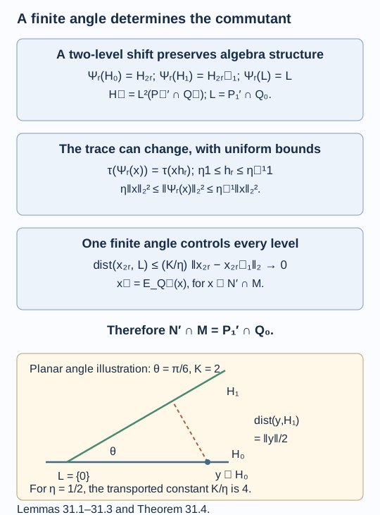
Figure 31.1. The maps carry onto . The squared norm bounds have constants ; the resulting distance constant is . Martingale adjacency tends to zero, so (31.13) forces . The lower drawing illustrates (31.12) for a planar angle, not a model of the algebras. Editable figure source.
Every higher relative commutant is finite data
Write , and let be the -th vertical basic-construction row from Proposition 30.5. Its limit is , where .
Corollary 31.5. For every , and for in the second formula,
These identifications preserve inclusions, restricted traces, expectations and the marked vertical Jones projections.
Proof. Compose the vertical squares from to . Each constituent square is commuting and nondegenerate by Proposition 30.5. Composite expectations still commute, and products of the transported frames span the composite square. Its horizontal Markov modulus remains ; summing the left index products of a product frame multiplies the scalar index elements, giving finite vertical modulus . Its limits are , so Theorem 31.4 gives the first formula. For the second, start the composite at the original row. Its limits are , and the same argument applies.
All equalities are equalities of subalgebras inside the actual tower constructed in lesson 30. Inclusions and traces are therefore inherited, rather than newly assigned. Its vertical expectations agree with the finite ones on every finite row, and its Jones projections are the same fixed finite projections. This proves the remaining assertions.
Thus a candidate finite grid becomes an actual standard invariant once its initial squares and its finite commutants are checked. For a grid defined by connection coefficients, one must still prove nondegeneracy, trace compatibility and the precise identification of the finite commutants with the claimed flat path spaces. A graph and a numerical check of its coefficients do not establish those assertions.
Exercises
Exercise 31.1 — introductory. For the tensor inclusion in Exercise 30.2, identify , and check the answer in the limit.
Solution. Here , is the next tensor factor, and is the first factor. They commute, so the finite commutant is . The limit is . Since is a factor, its commutant inside this tensor product consists exactly of the first factor, as predicted by (31.11).
Exercise 31.2 — intermediate. For as the diagonal algebra with normalized trace, compute the central transfer and all .
Solution. The size vector is , the inclusion matrix is , and has all four entries one. Thus , , and for all . Formula (31.10) therefore makes the shift trace preserving. This is a special balanced case of the uniform estimate.
Exercise 31.3 — advanced. Take with
Choose the Markov trace. Show that the shift need not preserve it, and give an explicit uniform .
Solution. Here , , and . The central transfer matrix is . Thus
For the first central projection , (31.8) gives . In the comparison of Lemma 31.3, and . Consequently every component of every lies between and . We may take . The proof of compactness applies with this constant.
Exercise 31.4 — intermediate. In a planar Hilbert-space example, let be the horizontal line and make angle with it. What are and the optimal constant in (31.12)? If the shift estimate has , what constant transports the distance inequality?
Solution. The intersection is zero. For , its distance to is , so . The transported constant is . The square roots in the two norm comparisons multiply to , not . This is an angle illustration, not an assertion that these lines themselves form a commuting square of algebras.