Original text: CC0 1.0. Prerequisite proofs and component terms.

Compatible pairs and complex interpolation

CC0 1.0.

The scalar estimate uses the rectangle boundary maximum proof below. The complex Hahn–Banach and dual-norm proofs and closed-subspace quotient proof supply the stated Banach-space inputs; the scalar Cauchy and power-series proofs supply the analytic inputs.

Interpolation arguments in modular theory act on two endpoint spaces at once. The endpoints need not be nested, reflexive, separable, or dense in one another. What is needed is a common Hausdorff ambient space, a precise sum norm, and an analytic strip class whose boundary values decay in the endpoint norms.

This unit constructs that framework from the ground up. It proves completeness of the intersection, sum, strip, and interpolation spaces and proves the exact geometric-mean bound for a linear map bounded at both endpoints. The mathematical antecedent is Takesaki, Theory of Operator Algebras II, Appendix A.12.

OA-MOD-CI-01 — Compatible pairs, intersections, and sums

A compatible pair is a pair $\mathbf X=(X_0,X_1)$ of complex Banach spaces with continuous injective linear maps into one Hausdorff topological vector space $\mathcal V$ . We identify each endpoint with its image. This identification matters: it gives a definite meaning to equality between an element of $X_0$ and an element of $X_1$ .

Set

\Delta(\mathbf X)=X_0\cap X_1,\qquad \Sigma(\mathbf X)=X_0+X_1

inside $\mathcal V$ , with

\|x\|_{\Delta} =\max\{\|x\|_{X_0},\|x\|_{X_1}\}, \tag{CI.1}

and

\|x\|_{\Sigma} =\inf_{x=x_0+x_1} \bigl(\|x_0\|_{X_0}+\|x_1\|_{X_1}\bigr). \tag{CI.2}

The infimum runs over $x_j\in X_j$ . In particular, the canonical maps $X_j\to\Sigma(\mathbf X)$ are contractions.

Proposition. Both $\Delta(\mathbf X)$ and $\Sigma(\mathbf X)$ are Banach spaces.

Proof. Let $(x_n)$ be Cauchy in $\Delta(\mathbf X)$ . It converges to some $x_j$ in $X_j$ for $j=0,1$ . Continuity of the two ambient embeddings makes the same sequence converge to $x_0$ and $x_1$ in $\mathcal V$ . Since $\mathcal V$ is Hausdorff, $x_0=x_1$ . The common vector lies in the intersection, and convergence holds in the maximum norm.

For the sum, give $X_0\oplus X_1$ the norm

\|(x_0,x_1)\|_{\oplus}=\|x_0\|_{X_0}+\|x_1\|_{X_1}.

This is a Banach space. The addition map

A:X_0\oplus X_1\longrightarrow\mathcal V,\qquad A(x_0,x_1)=x_0+x_1,

is continuous. Its kernel is closed because $\mathcal V$ is Hausdorff. Hence $(X_0\oplus X_1)/\ker A$ is Banach. The induced bijection from this quotient to $\Sigma(\mathbf X)$ has quotient norm exactly (CI.2), so it is an isometric isomorphism. $\square$

No norm on the ambient space is used. Different compatible realizations can therefore lead to different intersections and sums even when the abstract endpoint Banach spaces are isomorphic.

OA-MOD-CI-02 — The bounded-strip estimate

Write

\begin{aligned} \mathbb S &=\{z\in\mathbb C:0\leq\operatorname{Re}z\leq1\},\\ \mathbb S^\circ &=\{z\in\mathbb C:0<\operatorname{Re}z<1\}. \end{aligned}

We use the following form of the three-lines argument.

Lemma. Let $h:\mathbb S\to\mathbb C$ be bounded and continuous, and holomorphic on $\mathbb S^\circ$ . If

|h(it)|\leq a_0,\qquad |h(1+it)|\leq a_1 \quad(t\in\mathbb R),

then, for $0\leq s\leq1$ ,

|h(s+it)|\leq a_0^{\,1-s}a_1^{\,s} \quad(t\in\mathbb R). \tag{CI.3}

At an interior point, the right side is interpreted as zero when one endpoint bound is zero.

Proof. First suppose $a_0a_1>0$ . Fix $\varepsilon>0$ and use the real logarithms of $a_0,a_1$ to define

H_\varepsilon(z) =h(z)a_0^{z-1}a_1^{-z} \exp\bigl(\varepsilon(z^2-z)\bigr).

On either vertical boundary, its modulus is at most $\exp(-\varepsilon t^2)$ . If $|h|\leq C$ on the strip, then on either horizontal edge $z=s\pm iR$ ,

|H_\varepsilon(z)| \leq C\max(a_0^{-1},a_1^{-1})e^{-\varepsilon R^2},

because $s^2-s\leq0$ . For sufficiently large $R$ , the boundary maximum principle on the rectangle with vertices $\pm iR$ and $1\pm iR$ gives $|H_\varepsilon|\leq1$ throughout that rectangle. Evaluating at $s+it$ , then letting $\varepsilon\downarrow0$ , proves (CI.3). Replacing $a_j$ by $a_j+\delta$ and sending $\delta\downarrow0$ handles a zero endpoint bound. The endpoint cases follow directly from the hypotheses. $\square$

The proof uses boundedness on the full strip. Without a growth condition, the two boundary lines alone do not control a holomorphic function on an unbounded strip.

OA-MOD-CI-03 — The strip space is complete

For a compatible pair $\mathbf X=(X_0,X_1)$ , let $\mathcal F(\mathbf X)$ consist of functions

f:\mathbb S\longrightarrow\Sigma(\mathbf X)

with all of the following properties:

$f$ is bounded and continuous in the sum norm on $\mathbb S$ ;
$f$ is holomorphic in the sum norm on $\mathbb S^\circ$ ;
$f(j+it)\in X_j$ for $j=0,1$ and every real $t$ ;
each boundary map $t\mapsto f(j+it)$ is continuous as an $X_j$ -valued map and tends to zero in $X_j$ as $|t|\to\infty$ .

Put

\|f\|_{\mathcal F} =\max_{j=0,1}\sup_{t\in\mathbb R}\|f(j+it)\|_{X_j}. \tag{CI.4}

Let

A_j(f)=\sup_t\|f(j+it)\|_{X_j}.

For every $z=s+it\in\mathbb S$ ,

\|f(z)\|_{\Sigma} \leq A_0(f)^{\,1-s}A_1(f)^{\,s} \leq\|f\|_{\mathcal F}. \tag{CI.5}

Indeed, if $\ell\in\Sigma(\mathbf X)^*$ has norm at most one, then $\ell\circ f$ satisfies OA-MOD-CI-02, since

|\ell(f(j+it))| \leq\|f(j+it)\|_{\Sigma} \leq\|f(j+it)\|_{X_j}.

The complex Hahn–Banach theorem identifies the norm of $f(z)$ with the supremum over these functionals and gives (CI.5).

Theorem. The normed space $\mathcal F(\mathbf X)$ is complete.

Proof. Let $(f_n)$ be Cauchy for (CI.4). On each boundary it is uniformly Cauchy in $X_j$ . Completeness of $X_j$ gives a uniform limit

g_j\in C_0(\mathbb R;X_j).

Applying (CI.5) to $f_n-f_m$ shows that $(f_n)$ is uniformly Cauchy on the whole strip in $\Sigma(\mathbf X)$ . Let $f$ be its uniform sum-norm limit. It is bounded and continuous. Since the endpoint inclusions into the sum space are contractive, its boundary values agree with $g_j$ , so conditions 3 and 4 hold.

It remains to justify holomorphy without silently replacing weak convergence by norm convergence. Choose a closed disk contained in $\mathbb S^\circ$ . For each $n$ , the Banach-valued Cauchy formula on its boundary follows from the scalar formula: apply any $\ell\in\Sigma(\mathbf X)^*$ , and then use Hahn–Banach to recover equality of the vectors. The boundary integral exists as a Banach-valued Riemann integral because continuous curves are uniformly approximable by step functions. Uniform convergence permits passage to the limit in that formula. Expanding the Cauchy kernel on every smaller concentric disk gives a norm-convergent power series for $f$ . Thus $f$ is holomorphic.

Finally, $f_n\to f$ uniformly in $X_j$ on each boundary, so $\|f_n-f\|_{\mathcal F}\to0$ . $\square$

This proof also explains why the topology in the definition cannot be left implicit: interior convergence takes place in $\Sigma(\mathbf X)$ , while the stronger endpoint norms control the boundary.

OA-MOD-CI-04 — Evaluation spaces and quotient completeness

Fix $0<\theta<1$ . Define

[X_0,X_1]_\theta =\{f(\theta):f\in\mathcal F(\mathbf X)\} \subseteq\Sigma(\mathbf X)

and

\|x\|_\theta =\inf\{\|f\|_{\mathcal F}:f\in\mathcal F(\mathbf X),\ f(\theta)=x\}. \tag{CI.6}

The evaluation map

E_\theta:\mathcal F(\mathbf X)\longrightarrow\Sigma(\mathbf X), \qquad E_\theta f=f(\theta),

has norm at most one by (CI.5). Hence

K_\theta=\ker E_\theta

is closed. The induced map

\mathcal F(\mathbf X)/K_\theta \longrightarrow [X_0,X_1]_\theta

is an isometric bijection when the range is given (CI.6). Consequently $[X_0,X_1]_\theta$ is a Banach space. In particular, (CI.6) is a norm rather than only a seminorm, and

\|x\|_{\Sigma}\leq\|x\|_\theta. \tag{CI.7}

The intersection embeds in every interpolation space. More precisely, if $x\in X_0\cap X_1$ , then

\|x\|_\theta \leq \|x\|_{X_0}^{\,1-\theta}\|x\|_{X_1}^{\,\theta}. \tag{CI.8}

For nonzero $x$ , put $a=\|x\|_{X_0}$ , $b=\|x\|_{X_1}$ . For $\varepsilon>0$ , the function

f_\varepsilon(z) =e^{\varepsilon(z-\theta)^2} a^{z-\theta}b^{\theta-z}x

belongs to $\mathcal F(\mathbf X)$ , takes the value $x$ at $\theta$ , and has boundary norm at most

a^{1-\theta}b^\theta \max\{e^{\varepsilon\theta^2}, e^{\varepsilon(1-\theta)^2}\}.

Letting $\varepsilon\downarrow0$ gives (CI.8). The Gaussian factor is needed: the constant analytic representative does not decay along the boundary and therefore does not belong to this version of $\mathcal F$ .

OA-MOD-CI-05 — Interpolating a bounded linear map

Let $\mathbf X=(X_0,X_1)$ and $\mathbf Y=(Y_0,Y_1)$ be compatible pairs. Suppose

T:\Sigma(\mathbf X)\longrightarrow\Sigma(\mathbf Y)

is linear and

\|Tx\|_{Y_j}\leq M_j\|x\|_{X_j} \quad(x\in X_j,\ j=0,1) \tag{CI.9}

for positive constants $M_0,M_1$ .

First, $T$ is bounded between the sum spaces. If $x=x_0+x_1$ , then

\|Tx\|_{\Sigma(\mathbf Y)} \leq M_0\|x_0\|_{X_0}+M_1\|x_1\|_{X_1} \leq\max(M_0,M_1) \bigl(\|x_0\|_{X_0}+\|x_1\|_{X_1}\bigr).

Taking the infimum proves the assertion. Therefore $Tf\in\mathcal F(\mathbf Y)$ whenever $f\in\mathcal F(\mathbf X)$ .

Interpolation theorem. For every $0<\theta<1$ ,

T[X_0,X_1]_\theta\subseteq[Y_0,Y_1]_\theta

and

\|Tx\|_{[Y_0,Y_1]_\theta} \leq M_0^{\,1-\theta}M_1^{\,\theta} \|x\|_{[X_0,X_1]_\theta}. \tag{CI.10}

Proof. Given $f\in\mathcal F(\mathbf X)$ , define

g(z)=M_0^{z-1}M_1^{-z}Tf(z). \tag{CI.11}

The scalar factor is bounded on the strip. On the left boundary its modulus is $M_0^{-1}$ , and on the right boundary it is $M_1^{-1}$ . Thus (CI.9) gives

\|g\|_{\mathcal F(\mathbf Y)} \leq\|f\|_{\mathcal F(\mathbf X)}.

If $f(\theta)=x$ , then

g(\theta)=M_0^{\theta-1}M_1^{-\theta}Tx.

Definition (CI.6) therefore yields

\|Tx\|_{[Y_0,Y_1]_\theta} \leq M_0^{1-\theta}M_1^\theta\|f\|_{\mathcal F(\mathbf X)}.

Take the infimum over all representatives $f$ of $x$ . $\square$

If an endpoint bound is zero, apply (CI.10) with $M_j+\delta$ and let $\delta\downarrow0$ . No density of $X_0\cap X_1$ , reflexivity, or separability enters the proof.

OA-MOD-CI-06 — Checks and solved exercises

Check 1: identical endpoints. Suppose $X_0=X_1=X$ , with the same norm and the same ambient embedding. Then

[X,X]_\theta=X \quad\text{isometrically}.

Inequality (CI.7) gives $\|x\|_X\leq\|x\|_\theta$ , while (CI.8) gives the reverse inequality. This also checks that the boundary-decay convention has not changed the expected constant-endpoint space.

Check 2: a one-dimensional weighted pair. Let both endpoints be $\mathbb C$ in the usual ambient line, with

\|z\|_{X_0}=a|z|,\qquad \|z\|_{X_1}=b|z|,

where $a,b>0$ . Then

\|z\|_\theta=a^{1-\theta}b^\theta|z|.

The upper bound is (CI.8). For the lower bound, apply (CI.3) to any representative $f$ after multiplying its endpoint bounds by $a$ and $b$ :

a^{1-\theta}b^\theta|f(\theta)| \leq\|f\|_{\mathcal F}.

Taking the infimum gives equality. This model verifies both exponents and the direction of the scaling in (CI.11).

Exercise 1. Let $\varphi$ be a bounded scalar function continuous on the closed strip and holomorphic on its interior. Prove that multiplication by $\varphi$ maps $\mathcal F(\mathbf X)$ boundedly into itself, with norm at most $\max_{j=0,1}\sup_{t\in\mathbb R}|\varphi(j+it)|$ .

Solution. For $f\in\mathcal F(\mathbf X)$ , the product $\varphi f$ is bounded and continuous in the sum norm on the closed strip and holomorphic in its interior. Its endpoint values are continuous in each endpoint norm, and they decay there because $\varphi$ is bounded and $f$ decays. On boundary $j$ , $\sup_t\|\varphi(j+it)f(j+it)\|_{X_j} \leq\sup_t|\varphi(j+it)|\sup_t\|f(j+it)\|_{X_j}.$ Taking the maximum of the two boundary bounds proves the claimed operator norm.

Exercise 2. Let $S:\Sigma(\mathbf X)\to\Sigma(\mathbf Y)$ and $T:\Sigma(\mathbf Y)\to\Sigma(\mathbf Z)$ satisfy endpoint bounds $(A_0,A_1)$ and $(B_0,B_1)$ . Show that the interpolated bound for $TS$ obtained in one step agrees with the product of the two separate interpolated bounds.

Solution. The endpoint bounds for the composition are $(B_0A_0,B_1A_1)$ . Formula (CI.10) gives $(B_0A_0)^{1-\theta}(B_1A_1)^\theta = \bigl(B_0^{1-\theta}B_1^\theta\bigr) \bigl(A_0^{1-\theta}A_1^\theta\bigr).$ This is exactly the product of the separate operator-norm estimates.

The unit supplies the compatible-pair interpolation machinery only. Applications to noncommutative $L^p$ -spaces must still prove that the proposed endpoints form compatible pairs and that the operator acts consistently on their sum.

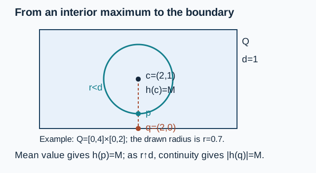
Nested circles at an interior maximum reach a nearest rectangle boundary point — Example coordinates are shown; the proof uses an arbitrary rectangle and 0<r<d. After rotating h(c) to M, the scalar mean-value identity makes h constant on each circle. The points approaching q transfer the maximum to the boundary. Exact proof: Rectangle boundary maximum; earlier scalar source: the linked programme Cauchy and power-series proofs.

Rectangle boundary maximum

Statement. Let $Q$ be a nondegenerate closed rectangle in the complex plane. If $h$ is continuous on $Q$ and holomorphic in its interior, the maximum of $|h|$ on $Q$ occurs on its boundary.

Proof. Compactness gives a maximum $M$ . If it is attained on the boundary, or if $M=0$ , the assertion holds. Otherwise let $c$ be an interior maximum point, let $d>0$ be its distance from the boundary, and choose a boundary point $q$ at distance $d$ . For every $0<r<d$ , the circle with centre $c$ and radius $r$ lies in the interior. The scalar Cauchy mean-value identity gives $h(c)$ as the average of $h$ on this circle. Multiply by a unimodular scalar so that $h(c)=M$ . The continuous nonnegative function $M-\operatorname{Re}h$ on the circle has integral zero, because its average is $M-\operatorname{Re}h(c)=0$ ; it therefore vanishes everywhere. Since $|h|\leq M$ , the value of $h$ everywhere on that circle is $M$ . The point $c+(r/d)(q-c)$ consequently has modulus $M$ . Let $r$ increase to $d$ . Continuity at $q$ gives $|h(q)|=M$ , proving the boundary assertion. The mean-value identity follows from the linked scalar Cauchy and power-series proofs. $\square$

Editable source · Proof dependencies and component terms