Trace-scaling cocycles and fixed corners

A unitary cocycle changes an action by a moving inner automorphism. For a real action that scales a faithful trace, this moving change comes from a single unitary. We prove that assertion by placing the original and perturbed actions in two corners of one matrix algebra.

The fixed algebra of that matrix action contains the desired unitary as an off-diagonal entry. Scalar Fourier averages detect both supports of that corner. Traces on central pieces then resolve the finite part of the comparison, while countable amplification handles the properly infinite part. These two arguments cover an arbitrary von Neumann algebra.

Original exposition, examples, figures, data and reproducible drawing code in this lesson are dedicated to CC0-1.0. Source publications and font components retain their own terms.

The action, the cocycle and the conclusion

Let $N\ne0$ be a von Neumann algebra with a faithful normal semifinite trace $\tau$. Let $\theta:\mathbb R\to\operatorname{Aut}(N)$ be a normal point-ultraweakly continuous action satisfying $\tau(\theta_s(x))=e^{-s}\tau(x) \qquad(s\in\mathbb R,\ x\in N_+). \tag{CST0.a}$ The equality includes infinite values. By AT1, the action is also point-strong-star continuous. Let $c:\mathbb R\to\mathcal U(N)$ be strongly continuous and satisfy $c_{s+t}=c_s\theta_s(c_t) \qquad(s,t\in\mathbb R). \tag{CST0.b}$ This identity forces $c_0=1$. Strong continuity of unitary fields also gives strong continuity of their adjoints; ST2 identifies this bounded topology intrinsically, so the condition does not depend on the chosen faithful normal representation.

We prove that there is a single $v\in\mathcal U(N)$ with $\boxed{\ c_s=v^*\theta_s(v)\quad(s\in\mathbb R).\ } \tag{CST0.c}$ Thus the perturbed action $\theta_s^c=\operatorname{Ad}(c_s)\theta_s$ satisfies $\boxed{\ \theta_s^c =\operatorname{Ad}(v^*)\,\theta_s\,\operatorname{Ad}(v).\ } \tag{CST0.d}$ Here $\operatorname{Ad}(v)(x)=vxv^*$, and products of maps mean composition with the rightmost map applied first. If one implementer $v$ has been chosen, the complete set of implementers is $\{\,hv:h\in\mathcal U(N^\theta)\,\}, \qquad N^\theta=\{x:\theta_s(x)=x\text{ for every }s\}. \tag{CST0.e}$

The cocycle need not be central or commutative. There is no assumption that $N$ is a factor, properly infinite, type III, countably decomposable, or has a separable predual. A faithful normal state is not needed. The fixed algebra introduced in Section 1 may have both semifinite and type III central parts.

Throughout this proof the action integral uses ordinary Lebesgue measure $ds$. The scalar Fourier transform of an integrable function is $\widehat f(r)=\int e^{-irs}f(s)\,ds$; only its uniqueness and continuity are used. No $1/(2\pi)$ is inserted into the action average.

The proof uses the full trace-scaling action integral, composition of normal operator-valued weights, tracial densities, modular restriction, scalar Fourier uniqueness, and projection comparison. The finite-center trace argument supplies the precise localization needed when total trace values are infinite. Their proofs occur earlier, and the point of use below specifies the required conclusion.

The zero algebra has its unique zero-algebra interpretation. None of the statements makes a measurable or continuous choice of $v$ as the cocycle $c$ varies.

1. Put the cocycle between two fixed corners

Let $N\ne0$ have a faithful normal semifinite trace $\tau$, and let $\theta:\mathbb R\to\operatorname{Aut}(N)$ be a normal strongly continuous action satisfying $\tau\circ\theta_s=e^{-s}\tau$ on $N_+$. Fix a strongly continuous unitary cocycle $c_{s+t}=c_s\theta_s(c_t)$. Its values need not commute. All assertions below allow an arbitrary center and arbitrary Hilbert multiplicity.

We use $e_{ij}$ for the standard matrix units in $M_2(N)$, with their nonzero entry equal to $1_N$. Define $\begin{gathered} A=M_2(N),\qquad T(X)=\tau(X_{11})+\tau(X_{22})\quad(X\in A_+),\\ d_s=\begin{pmatrix}1&0\\0&c_s\end{pmatrix},\qquad \alpha_s=\operatorname{Ad}(d_s)\circ(\operatorname{id}_2\otimes\theta_s),\\ F=A^\alpha,\qquad p=e_{11},\quad q=e_{22}. \end{gathered} \tag{CST1.a}$ Here and throughout, $\operatorname{Ad}(u)(x)=uxu^*$. The identity $d_{s+t}=d_s(\operatorname{id}_2\otimes\theta_s)(d_t)$ proves $\alpha_{s+t}=\alpha_s\alpha_t$. Also $c_0=1$, so $\alpha_0=\operatorname{id}$ and $\alpha_{-s}$ is the inverse of $\alpha_s$. Normality follows entrywise and from bounded conjugation. Strong continuity of a unitary path implies strong continuity of its adjoint, since $\|(c_s^*-c_t^*)\xi\|=\|(c_t-c_s)c_t^*\xi\|$. Bounded strong-star multiplication and AT1, AT4 therefore give point-strong-star, and hence point-ultraweak, continuity of $\alpha$. This is the continuity hypothesis of the action-integral theorem.

The full-cone construction in TW2, with the two-dimensional usual trace, makes $T$ faithful normal semifinite. It is a trace: for $Y=(y_{ij})$, $T(Y^*Y)=\sum_{i,j=1}^2\tau(y_{ij}^*y_{ij}) =\sum_{i,j=1}^2\tau(y_{ij}y_{ij}^*)=T(YY^*).$ Every sum here is nonnegative, so infinite values are retained. Tracial invariance under $d_s$, followed by the given scaling, gives $T\circ\alpha_s=e^{-s}T,\qquad \alpha_s(p)=p,\quad\alpha_s(q)=q. \tag{CST1.b}$ The fixed algebra $F$ is a von Neumann algebra, since it is the intersection of the ultraweakly closed fixed spaces of the normal maps $\alpha_s$.

Why use these particular diagonal positions? Every $w\in pAq$ is uniquely $w=e_{12}v$, with $v\in N$. Direct multiplication gives $\alpha_s(e_{12}v)=e_{12}\theta_s(v)c_s^*.$ Consequently, $\begin{gathered} w\in pFq,\qquad ww^*=p,\quad w^*w=q\\ \Longrightarrow\quad v\in\mathcal U(N),\qquad \theta_s(v)c_s^*=v,\qquad c_s=v^*\theta_s(v). \end{gathered} \tag{CST1.c}$ Conversely any unitary satisfying the last identity gives such a $w$. Thus the cocycle problem is exactly the equivalence of $p$ and $q$ inside $F$.

By L19, Section 1 and Section 2, the scaled trace in (CST1.b) supplies the faithful normal semifinite operator-valued weight $E:A_+\longrightarrow\widehat F_+,\qquad E(x)=\int_{\mathbb R}\alpha_s(x)\,ds =\sup_{m\ge1}\int_{-m}^m\alpha_s(x)\,ds. \tag{CST1.d}$ The supremum is in the extended positive cone. More explicitly, for every $\rho\in A_*^+$, $E(x)(\rho)=\int_{\mathbb R}\rho(\alpha_s(x))\,ds.$ Its finite spectral projections belong to $F$; this is the meaning of its target $\widehat F_+$. It satisfies $E\alpha_t=E$ and $E(b^*xb)=b^*E(x)b$ for $b\in F$. The cited proof first constructs the normal compact-interval maps, and then proves semifiniteness from an arbitrary-cardinality wandering partition. Thus no faithful normal state or countable decomposition of $N$ is being used. The measure in (CST1.d) is exactly Lebesgue measure $ds$.

2. An invariant density generates the whole linking algebra

Choose any faithful normal semifinite weight $\omega$ on $F$, whose existence at this scope is proved in FR1. The extension in EP5 and composition theorem EP6 make $\Psi=\widehat\omega\circ E$ a faithful normal semifinite weight on $A$, invariant under every $\alpha_s$. By TD4–6 it has a unique nonsingular positive self-adjoint density $H$ affiliated with $A$, characterized on the entire positive cone by $\Psi(x)=T_H(x) =\sup_{n\ge1}T\bigl(x^{1/2}(H\wedge n)x^{1/2}\bigr). \tag{CST2.a}$ TD6 proves that semifiniteness removes an infinite-value spectral summand and faithfulness removes the kernel. Neither centrality nor trace-measurability of $H$ is required.

For a normal automorphism $\beta$ with $T\circ\beta=aT$, $a>0$, normal transport of the bounded spectral cutoffs gives $T_H\circ\beta=T_{a\beta^{-1}(H)}$ on all positives. This is the full-cone calculation of L19, Section 3. Apply it to $\alpha_s$, use invariance of $\Psi$, and invoke TD5's uniqueness. It follows that $\alpha_s(H)=e^{-s}H,\qquad P=\log H,\qquad \alpha_s(P)=P-s1. \tag{CST2.b}$ The logarithm and this transported equality have their full affiliated-operator meaning from SF's spectral calculus.

The modular group of $T$ is trivial by the whole-cone trace criterion. The unbounded density formula CZ5 and the operator-valued modular restriction OT5 therefore give $\sigma_t^\Psi(x)=H^{it}xH^{-it}\quad(x\in A),\qquad H^{it}yH^{-it}=\sigma_t^\omega(y)\quad(y\in F). \tag{CST2.c}$ We next prove directly that $F$ together with these imaginary powers generates $A$.

An integrable spectral sandwich. Set $k(r)=\frac1{\sqrt{\pi(1+r^2)}},\qquad K_s=k(P-s1).$ The scalar function $k$ is strictly positive, belongs to $C_0(\mathbb R)$, and satisfies $\int_{\mathbb R}k(r)^2\,dr=1$. For any positive normal functional $\rho$, its finite spectral measure $\mu_\rho(B)=\rho(1_B(P))$ and scalar Tonelli give $\begin{aligned} \int_{\mathbb R}\rho(K_s^2)\,ds &=\int_{\mathbb R}\int_{\mathbb R}k(r-s)^2\,ds\,d\mu_\rho(r)\\ &=\rho(1). \end{aligned} \tag{CST2.d}$ In particular, in any faithful normal representation of $A$ on a Hilbert space $\mathcal K$, $\int\|K_s\xi\|^2ds=\|\xi\|^2$.

For $x\in A$, put $b_s=K_s\alpha_s(x)K_s =\alpha_s(k(P)xk(P)). \tag{CST2.e}$ Uniform continuity of $k$ makes $s\mapsto K_s$ norm continuous, and the action is point-strong-star continuous. Thus $b_s$ is a bounded strongly-star continuous path. For every interval $J\subset\mathbb R$, finite or infinite, vector Cauchy–Schwarz gives $\begin{aligned} \int_J|\langle b_s\xi,\eta\rangle|\,ds &\le\|x\| \left(\int_J\|K_s\xi\|^2ds\right)^{1/2} \left(\int_J\|K_s\eta\|^2ds\right)^{1/2}\\ &\le\|x\|\,\|\xi\|\,\|\eta\|. \end{aligned} \tag{CST2.f}$ The first inequality follows from the pointwise bound $|\langle\alpha_s(x)K_s\xi,K_s\eta\rangle| \le\|x\|\|K_s\xi\|\|K_s\eta\|$.

For fixed $r\in\mathbb R$, the identical estimate holds for each of $e^{-irs}b_s,\qquad e^{ir(P-s1)}b_s,\qquad b_s e^{ir(P-s1)}. \tag{CST2.g}$ Indeed the inserted unitary commutes with $K_s$. On the left it changes $K_s\eta$ to $e^{-ir(P-s1)}K_s\eta$; on the right it changes $K_s\xi$ to $e^{ir(P-s1)}K_s\xi$. The relevant norms do not change. This observation does not require that the unitary commute with $\alpha_s(x)$.

Here are the precise integral consequences. By CP4 and CP6, every $\varphi\in A_*$ is a series $\varphi(a)=\sum_j\langle a\xi_j,\eta_j\rangle$ with $\sum_j\|\xi_j\|\|\eta_j\|<\infty$. Applying (CST2.f) termwise, and then scalar nonnegative interchange, proves absolute integrability of every normal-functional test of each path in (CST2.g), as well as of $b_s$. The test functions are continuous: a finite part of the vector series is continuous, and its tail is uniformly small by the common operator bound.

On a compact interval, scalar integration defines a bounded functional on $A_*$, and hence an actual element of $A=(A_*)^*$, by CP6. Vector testing and (CST2.f) improve its norm bound to $\|x\|$, independently of the interval. The absolutely convergent scalar limits over $[-m,m]$ therefore give a bounded functional of norm at most $\|x\|$ on $A_*$, hence again an element of $A$. These are the weak-star integrals used below. In particular, their construction uses neither a Bochner integral in the operator norm nor a separability assumption on $\mathcal K$ or $A_*$. Every normal bounded linear map passes through these integrals, since its preadjoint changes only the normal functional being tested.

Two different modulations. Define $\begin{aligned} \widehat b(r)&=\int_{\mathbb R}e^{-irs}b_s\,ds,\\ L_r(x)&=\int_{\mathbb R} \alpha_s(e^{irP}k(P)xk(P))\,ds,\\ R_r(x)&=\int_{\mathbb R} \alpha_s(k(P)xk(P)e^{irP})\,ds. \end{aligned} \tag{CST2.h}$ These expressions mean the weak-star integrals just constructed. They need not be written as the value of the positive-cone map $E$ at a nonpositive argument. Translation of $s$ in each scalar test, together with the action law, shows that $L_r(x)$ and $R_r(x)$ are fixed by $\alpha$. Covariance (CST2.b) gives their exact factor orders: $\begin{gathered} L_r(x),R_r(x)\in F,\qquad \|L_r(x)\|,\|R_r(x)\|,\|\widehat b(r)\|\le\|x\|,\\ L_r(x)=e^{irP}\widehat b(r),\qquad R_r(x)=\widehat b(r)e^{irP}. \end{gathered} \tag{CST2.i}$ For example, the integrand of $L_r(x)$ is $e^{ir(P-s1)}b_s=e^{-irs}e^{irP}b_s$. Moving its constant left factor out of the weak-star integral proves the first identity. For $R_r(x)$ the constant factor stays on the right.

Generation by scalar Fourier uniqueness. Put $B_0=W^*(F,H^{it}:t\in\mathbb R).$ All bounded spectral functions of $P$ lie in $B_0$. One way to see the affiliation explicitly is RF5's generator construction: the Laplace integral of $e^{itP}$ belongs to $B_0$, and recovers the resolvent and its unique self-adjoint generator. SF then puts every bounded spectral function there. From (CST2.i), $\widehat b(r)=e^{-irP}L_r(x)\in B_0$.

Suppose $\varphi\in A_*$ vanishes on $B_0$. The continuous function $f_\varphi(s)=\varphi(b_s)$ is in $L^1(\mathbb R)$, and $\int_{\mathbb R}e^{-irs}f_\varphi(s)\,ds =\varphi(\widehat b(r))=0\quad(r\in\mathbb R).$ Scalar Fourier uniqueness makes $f_\varphi$ zero almost everywhere. Its continuity makes it zero everywhere, in particular at $s=0$. The predual annihilator identity now gives $k(P)xk(P)\in B_0$.

To remove the sandwich, use the bounded spectral operators $f_n=1_{[1/n,\infty)}(k(P)),\qquad l_n=k(P)^{-1}f_n,\qquad \|l_n\|\le n.$ The inverse in this expression is restricted to $f_n$; thus $l_n\in B_0$ is bounded. Since $k$ is everywhere strictly positive, $f_n\uparrow1$. For every $x\in A$, $l_n[k(P)xk(P)]l_n=f_nxf_n\in B_0, \qquad f_nxf_n\longrightarrow x\quad\text{strongly-star}.$ The approximants have norm at most $\|x\|$. Their bounded strong-star convergence is ultraweak convergence by ST2, so the von Neumann algebra $B_0$ contains their limit. We have proved $A=W^*(F,H^{it}:t\in\mathbb R). \tag{CST2.j}$ Only scalar Fourier uniqueness was applied. Each normal functional was treated separately, and continuity supplied equality at the single required time; no common exceptional null set for an uncountable family of tests was chosen.

The center of the fixed algebra is central upstairs. The proof in NC4 shows that central elements commute with the full modular operator, so $\sigma_t^\omega(z)=z$ for $z\in Z(F)$. Equation (CST2.c) makes $z$ commute with every $H^{it}$. It already commutes with $F$, and (CST2.j) consequently gives $Z(F)\subseteq Z(A). \tag{CST2.k}$ In particular, any central projection used to decompose $F$ commutes with the original matrix units of $A$.

3. Countable support bounds for the two fixed corners

We now choose the reference weight in Section 2 so that its density respects the two corners. Choose faithful normal semifinite weights $\omega_p$ on $pFp$ and $\omega_q$ on $qFq$, by FR1, and set $\omega(y)=\omega_p(pyp)+\omega_q(qyq)\quad(y\in F_+). \tag{CST3.a}$ To check semifiniteness without a countability assumption, let $D=pFp\oplus qFq$ and consider $\Delta:F\to D$, $\Delta(y)=pyp+qyq$. This is a bounded normal positive $D$-bimodule map, fixes $D$, and is faithful: if $y\ge0$ and both diagonal compressions vanish, then $y^{1/2}p=y^{1/2}q=0$, hence $y=0$. Its operator-valued finite ideal is all of $F$. The direct-sum weight on $D$ is faithful normal semifinite, since the two finite ideals are dense in their respective corners. Thus EP6 proves that (CST3.a) is faithful normal semifinite on $F$.

Let $H$ be the density of $\Psi=\widehat\omega\circ E$ for this choice. The self-adjoint unitary $j=p-q$ belongs to $F$. The diagonal formula makes $\omega\circ\operatorname{Ad}(j)=\omega$, and bimodularity of $E$ makes $\Psi\circ\operatorname{Ad}(j)=\Psi$. Since $T\circ\operatorname{Ad}(j)=T$, the full-cone density covariance and uniqueness used in (CST2.b) give $jHj=H$. Hence $p$ and $q$ reduce all its spectral projections, and $H=\begin{pmatrix}h_1&0\\0&h_2\end{pmatrix},\qquad P=\begin{pmatrix}P_1&0\\0&P_2\end{pmatrix},\qquad P_i=\log h_i. \tag{CST3.b}$ Here $h_1,h_2$ are nonsingular positive self-adjoint operators affiliated with $N$. They act in the same faithful representation of $N$, but need not commute with one another.

Apply (CST2.e)–(CST2.i) to $x=e_{12}$. Because $p,q$ are fixed and commute with the spectral functions of $P$, all $b_s,L_r(x),R_r(x)$ belong to $pAq$, and the last two belong to $pFq$. At $s=0$ the upper-right entry is exactly $b_0=e_{12}k(P_1)k(P_2). \tag{CST3.c}$ Each $k(P_i)$ is bounded, self-adjoint and injective: its kernel is the spectral projection of the empty zero set of $k$. Thus $k(P_1)k(P_2)$ is injective. Its adjoint $k(P_2)k(P_1)$ is also injective, which makes its range dense. In corner language, the right support of $b_0$ is $q$ and its left support is $p$.

For an operator $a$, write $s_r(a)$ and $s_l(a)$ for the initial and final projections of its polar part, respectively. Their existence in the same von Neumann algebra is PC1. We claim $\bigvee_{r\in\mathbb Q}s_r(L_r(e_{12}))=q,\qquad \bigvee_{r\in\mathbb Q}s_l(R_r(e_{12}))=p. \tag{CST3.d}$ For the first assertion let $a\le q$ be the complement in $q$ of the displayed join. Then $L_r(e_{12})a=0$ for every rational $r$. The first factorization in (CST2.i) permits multiplication by $e^{-irP}$ on the left, giving $\widehat b(r)a=0$.

For each $\varphi\in A_*$, the scalar function $s\mapsto\varphi(b_sa)$ is continuous and integrable: right multiplication by $a$ is normal, so it is another test of the integrable path already proved. Its Fourier transform is $\varphi(\widehat b(r)a)$. This transform is continuous in $r$, by scalar dominated convergence, and vanishes on the dense set $\mathbb Q$. It therefore vanishes on $\mathbb R$. Fourier uniqueness followed by time continuity gives $\varphi(b_0a)=0$. Normal functionals separate $A$, so $b_0a=0$; the right support in (CST3.c) forces $a=0$.

For the second assertion let $a\le p$ be the complement of the left-support join. Now $aR_r(e_{12})=0$. The second factorization in (CST2.i) permits cancellation of $e^{irP}$ on the right, giving $a\widehat b(r)=0$ for rational $r$. Apply the same scalar argument to $s\mapsto\varphi(ab_s)$. It gives $ab_0=0$, and the dense range in (CST3.c) forces $a=0$. This is why the left and right modulations were both constructed. Cancelling the left unitary after an arbitrary left annihilator, or the right unitary before an arbitrary right annihilator, would have required an unavailable commutation relation.

Turn support joins into actual comparisons. Enumerate $\mathbb Q=\{r_n:n\ge1\}$. Let $(\varepsilon_{ij})$ be the standard matrix units of $B(\ell^2(\mathbb N))$, distinct from the linking matrix units $e_{ij}$. In $\mathscr M=F\bar\otimes B(\ell^2(\mathbb N))$, form $C_L=\sum_{n\ge1}2^{-n}L_{r_n}(e_{12})\otimes\varepsilon_{n1}, \qquad C_R=\sum_{n\ge1}2^{-n}R_{r_n}(e_{12})^*\otimes\varepsilon_{n1}. \tag{CST3.e}$ The tails of these series have norm at most $(\sum_{n>m}4^{-n})^{1/2}$, since the entries have norm at most one by (CST2.i). They therefore define actual elements of the normal matrix amplification, whose arbitrary-H construction is TW1.

The operator $C_L$ has right support $q\otimes\varepsilon_{11}$. Indeed its kernel on that input corner is the common kernel of the $L_{r_n}(e_{12})$, which is zero by (CST3.d); it vanishes on the complementary input corner. Its left support is at most $p\otimes1$. The polar decomposition in $\mathscr M$ therefore gives the first comparison below. Applying the same argument to $C_R$ gives the second: $q\otimes\varepsilon_{11}\precsim p\otimes1, \qquad p\otimes\varepsilon_{11}\precsim q\otimes1 \quad\text{inside }\mathscr M. \tag{CST3.f}$ These are countable amplification bounds. They do not assert that either $p$ or $q$ is countably decomposable.

Both corners also have full central support in $F$. For example, if $z\in Z(F)$ is a projection and $zp=0$, then $zL_r(e_{12})=0$. Centrality in $F$ gives $L_r(e_{12})zq=0$, and the first support join in (CST3.d) implies $zq=0$. Since $p+q=1$, this forces $z=0$. The other side follows using the second join. Thus $c_F(p)=c_F(q)=1. \tag{CST3.g}$ Multiplying the operators in (CST3.e) by any central projection $z$ preserves the support identities in the algebra $Fz$. Hence (CST3.f) and fullness hold on every nonzero central portion.

Properly infinite portions. Suppose $z\in Z(F)$ and both $pz$ and $qz$ are properly infinite. For the following construction work in $Fz$, temporarily writing $p,q$ for $pz,qz$ and using the centrally compressed columns. The filling-family theorem PC5 gives $v_n\in pFp$ such that $v_n^*v_m=\delta_{nm}p,\qquad \sum_{n\ge1}v_nv_n^*=p.$ The row $S_p=\sum_{n\ge1}v_n\otimes\varepsilon_{1n}$ converges strongly together with its adjoints. For the row, orthogonality bounds the tail on a vector by its $\ell^2$ input-coordinate tail; for the adjoint, the filling identity bounds it by the tail of $\sum_n\|v_n^*\xi\|^2=\|p\xi\|^2$. Its initial and final projections are $S_p^*S_p=p\otimes1,\qquad S_pS_p^*=p\otimes\varepsilon_{11}. \tag{CST3.h}$ Composing $S_p$ with the polar part of $C_L$ yields a partial isometry with initial projection $q\otimes\varepsilon_{11}$ and final projection at most $p\otimes\varepsilon_{11}$. It lies in the $\varepsilon_{11}$ corner and thus corresponds to an element of $Fz$; this proves $q\precsim p$ in $Fz$ itself. The filling row for $q$, composed with the polar part of $C_R$, proves $p\precsim q$. Applying PC3's mutual-subequivalence theorem and restoring the original notation gives $pz\sim qz\quad\text{whenever both }pz\text{ and }qz \text{ are properly infinite}. \tag{CST3.i}$ By PC8, every nonzero projection in a type III algebra is properly infinite, so this includes every type III central portion of $F$. The countable bounds (CST3.f), rather than fullness alone, justify the absorption at arbitrary cardinality. The remaining central portions require a finite-corner comparison, to which we now turn.

4. Equal trace values on every semifinite central piece

Retain the linking algebra and fixed algebra of Section 1: $A=M_2(N),\qquad F=A^\alpha,\qquad p=e_{11},\quad q=e_{22},\qquad E(x)=\int_{\mathbb R}\alpha_s(x)\,ds.$ Here $N\ne0$, the trace $\tau$ is faithful normal semifinite, and the normal continuous action satisfies $\tau\circ\theta_s=e^{-s}\tau$. The strongly continuous unitary cocycle may be noncentral. The matrix trace is $T=\operatorname{Tr}_2\otimes\tau$, and $T\circ\alpha_s=e^{-s}T$. The integral uses the fixed Lebesgue measure $ds$.

We will prove $\boxed{\ \rho(pz)=\rho(qz)\ } \quad\begin{gathered} z\in Z(F)\text{ a projection with }Fz\text{ semifinite},\\ \rho\text{ any faithful normal semifinite trace on }Fz. \end{gathered} \tag{CST4.1}$ All values are allowed to be infinite. The quantifiers over both the central piece and the trace will be needed: an equality only at the original unit would not detect a strict comparison hidden in a finite central cut.

Take a nonzero such $z$. By the center inclusion proved in Section 2, $z\in Z(A)$, and it is fixed by $\alpha$. Thus $A_z=Az$ has unit $z$, restricted action $\alpha^z$, fixed algebra $Fz$, and faithful normal semifinite trace $T_z=T|_{Az}$. The restricted action integral $E_z:(Az)_+\longrightarrow\widehat{Fz}_+, \qquad E_z(x)=E(x),$ is faithful normal semifinite by the action-integral construction in L19, Sections 1–2, applied to $(Az,T_z,\alpha^z)$. Trace restriction to a corner is semifinite by the compression argument in L18, Section 7.

Compose the chosen trace with this integral: $\Psi_\rho=\widehat\rho\circ E_z=(T_z)_{H_\rho}, \qquad P_\rho=\log H_\rho. \tag{CST4.2}$ The hat denotes the extension of a normal weight to the full extended positive cone. EP6 makes $\Psi_\rho$ faithful normal semifinite, and TD4–6 give its unique nonsingular positive self-adjoint density $H_\rho$ affiliated with $Az$. Apply the invariant-density and generation argument of Section 2, now with the reference weight $\rho$ on $Fz$. It gives $\alpha_s^z(H_\rho)=e^{-s}H_\rho,\qquad \alpha_s^z(P_\rho)=P_\rho-sz,\qquad Az=W^*(Fz,H_\rho^{it}:t\in\mathbb R). \tag{CST4.3}$ This use of generation is valid for each new reference weight; it does not assert that densities for different traces coincide.

Since $\rho$ is a trace, its modular group is trivial. The operator-valued-weight modular restriction and the tracial density modular formula therefore imply $H_\rho^{it}xH_\rho^{-it}=x\qquad(x\in Fz). \tag{CST4.4}$ Each $H_\rho^{it}$ also commutes with every $H_\rho^{iu}$. By the generation in (CST4.3), it is central in $Az$. The spectral recovery from the imaginary-power group then puts every spectral projection of $P_\rho$, and of $H_\rho$, in $Z(Az)$. Thus both operators are affiliated with that center. The same modular formula makes $\sigma^{\Psi_\rho}$ trivial on all of $Az$; the whole-cone trace criterion proves $\Psi_\rho(a^*a)=\Psi_\rho(aa^*)\qquad(a\in Az), \tag{CST4.5}$ including infinite values.

There is a bounded spectral window whose action integral is exactly the unit. Put $f=1_{[0,1]},\qquad g=f(P_\rho)\in Z(Az).$ The spectral measure $D_\rho$ of $P_\rho$ has total mass $z$. For any positive normal functional $\eta$ on $Az$, scalar spectral integration and Tonelli give $\begin{aligned} \int_{\mathbb R}\eta(\alpha_s^z(g))\,ds &=\int_{\mathbb R}\int_{\mathbb R} 1_{[0,1]}(r-s)\,d\eta(D_\rho(r))\,ds\\ &=\int_{\mathbb R} \left(\int_{\mathbb R}1_{[0,1]}(r-s)\,ds\right) d\eta(D_\rho(r)) =\eta(z). \end{aligned} \tag{CST4.6}$ The inner integral is one for every $r$. Endpoint choices do not change its Lebesgue value. The defining increasing bounded-interval integrals therefore have extended supremum equal to the bounded element $z$. Bimodularity of $E_z$, with $pz,qz\in Fz$, gives the exact identities $E_z(g)=z,\qquad E_z(pzg)=pz,\qquad E_z(qzg)=qz. \tag{CST4.7}$ For example, $pzg=(pz)g(pz)$ because $g$ is central. These equalities retain the measure $ds$ used throughout the proof.

Now take the bounded element $a=ze_{12}g\in Az$. Centrality and $g^2=g$ give $aa^*=pzg,\qquad a^*a=qzg.$ Equations (CST4.2), (CST4.5), and (CST4.7) yield $\rho(pz) =\Psi_\rho(aa^*) =\Psi_\rho(a^*a) =\rho(qz). \tag{CST4.8}$ This proves (CST4.1) for the arbitrary chosen pair $(z,\rho)$; the zero piece gives the zero equality. In particular, it applies again to every further central cut and the restriction of any such trace. No infinite trace values have been subtracted.

5. Central comparison, the implementing unitary, and all its choices

The countable support comparisons of Section 3 show that $p$ and $q$ have central support one in $F$, and already give their equivalence wherever both are properly infinite. To treat the remaining pieces, we need a finite value on a suitable central cut. Finiteness of a projection alone does not say that a given semifinite trace has a finite value on it.

Finite-center restriction. Let $D$ be a nonzero finite von Neumann algebra with a faithful normal semifinite trace $\lambda$. Then $\lambda|_{Z(D)}\text{ is faithful normal semifinite}. \tag{CST5.1}$ Here is the full argument from L18, Section 7, with the ingredients displayed. FCT6–7 constructs the normalized faithful normal center-valued trace $\mathcal T_D:D\to Z(D)$. Choose a faithful normal semifinite weight $\nu$ on $Z(D)$, using the arbitrary-algebra construction FR1. Because the center is commutative, $\nu$ is tracial. The map $\mathcal T_D$, viewed as an operator-valued weight, is faithful normal and semifinite: it is bounded, its bounded-value ideal is all of $D$, and its center-module law is the required bimodularity. Thus EP6 proves that $\lambda_0=\nu\circ\mathcal T_D$ is faithful normal semifinite. It is a trace on the entire positive cone because $\mathcal T_D(x^*x)=\mathcal T_D(xx^*)$.

The full tracial density theorem supplies a unique nonsingular affiliated $h$ with $\lambda=(\lambda_0)_h$. Both traces have trivial modular groups, so the modular formula makes every $h^{it}$ central. Spectral recovery makes $h$ affiliated with $Z(D)$, exactly as in the central trace-density proof. For $x\in Z(D)_+$, put $h_n=h\wedge n$. The whole-cone cutoff formula, centrality, and the normalization $\mathcal T_D|_{Z(D)}=\mathrm{id}$ give $\begin{aligned} \lambda(x) &=\sup_n\lambda_0(h_n^{1/2}xh_n^{1/2})\\ &=\sup_n\nu\bigl(\mathcal T_D(h_nx)\bigr) =\sup_n\nu(h_nx)=\nu_h(x). \end{aligned} \tag{CST5.2}$ The density $h$ is an ordinary nonsingular self-adjoint operator, so TD6, now on the commutative algebra $Z(D)$, proves that $\nu_h$ is faithful normal semifinite. This proves (CST5.1), with all extended values retained. The argument uses the constructed center-valued trace and density theorem; it needs no norm-closed unitary-orbit averaging theorem.

Strict comparison has a finite central witness. Let $B$ be a nonzero semifinite von Neumann algebra, let $a$ be a finite projection with $c_B(a)=1$, and let $b$ be a projection satisfying $a\precsim b$ but $a\not\sim b$. For every faithful normal semifinite trace $\rho$ on $B$, there is a nonzero central projection $z_0$ such that $\rho(az_0)<\infty,\qquad \rho(bz_0)>\rho(az_0). \tag{CST5.3}$ To prove this, choose $u\in B$ with $u^*u=a,\qquad a'=uu^*\le b,\qquad r=b-a'\ne0,\qquad t=c_B(r).$ The residual is nonzero because otherwise $u$ would implement $a\sim b$. The restriction $\rho_a=\rho|_{aBa}$ is faithful normal semifinite. In detail, if $y\in B_+$ and $\rho(y)<\infty$, the trace identity and order give $\rho(aya)=\rho(y^{1/2}ay^{1/2})\le\rho(y)<\infty. \tag{CST5.4}$ The finite positive cone of $\rho$ has ultraweakly dense linear span. Normal compression by $a$ makes the span of these finite positive compressions dense in $aBa$. Hence the finite-cone criterion GW4 proves semifiniteness of $\rho_a$; normality and faithfulness are inherited.

The algebra $aBa$ is finite, so (CST5.1) makes $\rho_a$ semifinite on $Z(aBa)$. Fullness of $a$ and $t\ne0$ give $at\ne0$. Consequently there is a nonzero positive $x\in Z(aBa)$, supported on $at$, with $\rho(x)<\infty$. Indeed the finite positive cone on the center has dense span, and compression by the nonzero central projection $at$ cannot annihilate that span. Choose $\delta>0$ with $e=1_{[\delta,\infty)}(x)\ne0.$ Then $e\in Z(aBa)$, $e\le at$, and $\rho(e)\le\delta^{-1}\rho(x)<\infty$.

The normal center isomorphism for a full corner, PC4, writes $e=az_0$ for a unique nonzero $z_0\in Z(B)$, with $z_0\le t$. The inequality follows because that isomorphism preserves order and takes $t$ to $at$. Also $rz_0\ne0$: a central projection annihilating $r$ is orthogonal to $c_B(r)=t$, whereas $0\ne z_0\le t$. Compressing $u$ by $z_0$ gives $az_0\sim a'z_0$, and therefore $\begin{aligned} \rho(bz_0) &=\rho(a'z_0)+\rho(rz_0)\\ &=\rho(az_0)+\rho(rz_0)>\rho(az_0), \qquad \rho(az_0)<\infty. \end{aligned} \tag{CST5.5}$ Faithfulness gives $\rho(rz_0)>0$. Its value may be infinite; adding it to the finite value $\rho(az_0)$ still gives the stated strict inequality. This proves (CST5.3) without canceling infinite values.

Refine the fixed algebra by its central pieces. The semifinite/type III construction in L18, Section 6 gives a central projection $z_{\mathrm{sf}}\in F$ such that $Fz_{\mathrm{sf}}$ admits a faithful normal semifinite trace and $F(1-z_{\mathrm{sf}})$ has no nonzero finite projections. The construction uses arbitrary orthogonal families of central pieces and finite-corner traces; it does not assume a faithful normal state on $F$. On the type III piece every nonzero projection is properly infinite by PC8. Thus Section 3 already gives $p(1-z_{\mathrm{sf}})\sim q(1-z_{\mathrm{sf}}) \quad\text{inside }F(1-z_{\mathrm{sf}}). \tag{CST5.6}$

Both $p$ and $q$ have full central support in $F$. Apply PC5's finite/properly infinite decomposition to each corner $pFp$ and $qFq$. By PC4, their central decompositions lift to central projections $z_p,z_q\in Z(F)$ with $\begin{array}{ll} pz_p\text{ finite},&p(1-z_p)\text{ properly infinite if nonzero},\\ qz_q\text{ finite},&q(1-z_q)\text{ properly infinite if nonzero}. \end{array} \tag{CST5.7}$ Intersect these two decompositions with $z_{\mathrm{sf}}$. On $z_{\mathrm{sf}}(1-z_p)(1-z_q)$, both sides are properly infinite, and Section 3 gives their equivalence. Each of the other three central pieces has at least one finite side. Every nonzero central compression of $p$ or $q$ is still full in the compressed algebra: a central subprojection annihilating that compression would annihilate the original full projection on that subpiece.

Fix one of these remaining nonzero pieces $y$, and put $B=Fy$. By PC2's central comparison, there is a central projection $e\le y$ such that $pe\precsim qe$ and $q(y-e)\precsim p(y-e)$. Consider either nonzero comparison part, with unit $y'$. Call the smaller projection $a$, the larger $b$. Both are full in $Fy'$. At least one is finite; if it is the larger one, the smaller one is finite too, because finiteness passes through equivalence and to subprojections by PC5. Thus in either case $a$ is finite.

Choose a faithful normal semifinite trace $\rho$ on $Fy'$, for example the restriction of one on $Fz_{\mathrm{sf}}$. If $a\not\sim b$, (CST5.3) supplies a nonzero central $z_0\le y'$ with $\rho(az_0)<\rho(bz_0)$. But $\{az_0,bz_0\}=\{pz_0,qz_0\}$. The restricted trace on $Fz_0$ is faithful normal semifinite, so Section 4 gives $\rho(pz_0)=\rho(qz_0)$, a contradiction. Therefore the two projections are equivalent on every comparison part. This also rules out any nonzero mixed finite/properly infinite piece, since equivalence preserves finiteness.

We have obtained $pz_j\sim qz_j$ on an orthogonal central partition $(z_j)$ of the unit of $F$. Each comparison and decomposition theorem used here holds at arbitrary cardinality. For clarity, the final assembly works for an arbitrary index set: choose $w_j\in pFq$ with $w_j^*w_j=qz_j,\qquad w_jw_j^*=pz_j.$ For any finite set $J$ of indices and any vector $\xi$ in the concrete Hilbert space of $A$, $\left\|\sum_{j\in J}w_j\xi\right\|^2 =\sum_{j\in J}\|qz_j\xi\|^2\le\|\xi\|^2.$ The supremum of these finite sums of nonnegative real numbers has arbitrarily small complementary finite tails; hence the vector sums are Cauchy. The same argument applies to adjoints, using $pz_j$. The arbitrary orthogonal-sum proof PC1 gives a strong-star sum in $F$: $w=\sum_jw_j\in pFq,\qquad w^*w=\sum_jqz_j=q,\qquad ww^*=\sum_jpz_j=p. \tag{CST5.8}$ No countable decomposition of the algebra has been chosen. On properly infinite pieces the crucial input was the two actual countable amplification comparisons of Section 3, followed by PC5's filling copies and PC3's mutual-subequivalence theorem. Full central support by itself was never used to identify arbitrary properly infinite projections.

Read the upper-right entry. Since $w\in pAq$, write $w=\begin{pmatrix}0&v\\0&0\end{pmatrix},\qquad v\in N.$ The initial and final projections in (CST5.8) give $v^*v=vv^*=1$, so $v$ is unitary. The linking action is $\alpha_s=\operatorname{Ad}\!\begin{pmatrix}1&0\\0&c_s\end{pmatrix} \circ(\operatorname{id}_2\otimes\theta_s).$ Its upper-right entry at $w$ is $\theta_s(v)c_s^*$. As $w\in F$, this equals $v$, and therefore $\boxed{\ c_s=v^*\theta_s(v)\qquad(s\in\mathbb R).\ } \tag{CST5.9}$ This proves stability for every strongly continuous unitary cocycle under the stated trace-scaling hypothesis, with no centrality, proper-infiniteness, factor, separability, countable-decomposability, or faithful-state assumption on $N$.

The cocycle perturbation $\theta_s^c=\operatorname{Ad}(c_s)\circ\theta_s$ is consequently inner conjugate to the original action. With the convention $\operatorname{Ad}(u)(x)=uxu^*$, for every $x\in N$, $\begin{aligned} \theta_s^c(x) &=v^*\theta_s(v)\theta_s(x)\theta_s(v^*)v\\ &=v^*\theta_s(vxv^*)v. \end{aligned}$ Hence $\boxed{\ \theta_s^c =\operatorname{Ad}(v^*)\circ\theta_s\circ\operatorname{Ad}(v).\ } \tag{CST5.10}$ The two inner automorphisms have this order; equivalently $\operatorname{Ad}(v)\circ\theta_s^c=\theta_s\circ\operatorname{Ad}(v)$.

All implementing unitaries. Define the fixed algebra $N^\theta=\{x\in N:\theta_s(x)=x\text{ for every }s\in\mathbb R\}.$ Once one $v$ satisfying (CST5.9) is chosen, the full set of solutions is the left coset $\boxed{\ \{u\in\mathcal U(N):c_s=u^*\theta_s(u)\text{ for all }s\} =\mathcal U(N^\theta)\,v. \ } \tag{CST5.11}$ Indeed, if $h\in\mathcal U(N^\theta)$, then $(hv)^*\theta_s(hv) =v^*h^*\theta_s(h)\theta_s(v) =v^*\theta_s(v)=c_s.$ Conversely, if $u$ is another solution, then $\theta_s(u)=uc_s$ and $\theta_s(v)=vc_s$. The unitary $h=uv^*$ satisfies $\theta_s(h)=uc_s(vc_s)^*=uv^*=h,$ so $h\in\mathcal U(N^\theta)$ and $u=hv$. Each such $h$ is uniquely determined by $u$ and the chosen $v$.

For $N=0$, the unit is $0$, its unitary group has its unique element, and the action, cocycle, implementer, and inner conjugacy all have their unique zero-algebra interpretation. Thus the conclusion includes that case as well.

6. Exact models and the boundaries of the argument

The theorem allows a finite von Neumann algebra with an infinite trace, noncommuting cocycle values, and an uncountable family of central summands. The following models separate these possibilities. Throughout the translation examples, the real variable is $q$, the action parameter is $s$, and the action integral uses $ds$.

Translation, its full trace, and scalar phases

For a positive integer $n$, let $\begin{aligned} N_n&=L^\infty(\mathbb R,e^q\,dq)\,\overline\otimes\,M_n(\mathbb C),\\ (\theta_s x)(q)&=x(q+s),\qquad \tau_n(x)=\int_{\mathbb R}e^q\operatorname{Tr}_n(x(q))\,dq \quad(x\in(N_n)_+). \end{aligned} \tag{CST6.1}$ Here $\operatorname{Tr}_n(I_n)=n$. The measure $e^q\,dq$ has the same null sets as Lebesgue measure, so translation is well defined on equivalence classes. Represent $N_n$ by multiplication on $\mathcal H_n=L^2(\mathbb R,e^q\,dq;\mathbb C^n)$. The operators $(U_s\xi)(q)=e^{s/2}\xi(q+s),\qquad U_sM_xU_s^*=M_{\theta_s x} \tag{CST6.2}$ are unitaries: the substitution $u=q+s$ proves equality of squared norms, and $U_{-s}$ is the inverse. On continuous compactly supported vectors they are norm continuous in $s$, by dominated convergence on a common compact interval; those vectors are dense, and the uniform unitary bound proves strong continuity on all of $\mathcal H_n$. Spatial conjugation is normal. For each bounded $x$, strong continuity of $U_s$ and $U_s^*$ proves point-strong-star continuity of $\theta$. In particular this is a normal continuous action, with the topology of AT1.

Each bounded-interval restriction of $\tau_n$ is a normal positive functional: its scalar matrix coefficients are integrable against $e^q\,dq$. Their increasing supremum is $\tau_n$, so it is normal, also for bounded increasing nets, by interchanging the two numerical suprema. Positivity of $e^q$ and faithfulness of the finite matrix trace prove faithfulness. The central projections $f_m=1_{[-m,m]}I_n$ increase to $1$, and $\tau_n(f_mxf_m)\le n\|x\|(e^m-e^{-m})<\infty$. These increasing compressions prove semifiniteness. Pointwise matrix cyclicity gives $\tau_n(a^*a)=\tau_n(aa^*)$, including infinity. Finally, for every bounded positive $x$, scalar substitution gives the full equality $\tau_n(\theta_s x) =\int_{\mathbb R}e^{u-s}\operatorname{Tr}_n(x(u))\,du =e^{-s}\tau_n(x). \tag{CST6.3}$ No finiteness of either integral is needed. In fact $\tau_n(1)=\infty$, while $N_n$ is finite in the projection sense: a pointwise isometry in $M_n$ is pointwise unitary, so an isometry in $N_n$ cannot have a proper final projection. Thus proper infiniteness of $N$ is not a premise of the theorem.

For $n=1$, fix $a,b\in\mathbb R$ and put $v(q)=\exp\!\left(i\left(\tfrac a2 q^2+bq\right)\right),\qquad c_s(q)=\exp\!\left(i\left(aqs+\tfrac a2s^2+bs\right)\right). \tag{CST6.4}$ Then $c_s=\overline v\,\theta_s(v)$. Expanding the exponent verifies $c_s(q)c_t(q+s) =\exp\!\left(i\left(aq(s+t)+\tfrac a2(s+t)^2+b(s+t)\right)\right) =c_{s+t}(q). \tag{CST6.5}$ For each vector $\xi\in\mathcal H_1$, pointwise continuity and the bound $4|\xi(q)|^2$ for the squared difference prove strong continuity of the multiplying unitaries $c_s$. The same argument applies to their adjoints. Uniform continuity of $v$ on the entire line is unnecessary.

The fixed algebra of translation is the constant matrices. One way to respect the equivalence-class issue is to convolve each bounded scalar entry with a smooth compactly supported approximate identity. Invariance under every translation in $L^\infty$ makes each convolution a continuous translation-invariant function, hence constant. The convolutions converge locally in $L^1$ to the entry; their constants converge on any interval of positive finite length, so the entry is constant almost everywhere. This is also the fixed-algebra conclusion in the earlier translation model. Consequently all scalar implementers in (CST6.4) are exactly $\lambda v$, $|\lambda|=1$, in agreement with Section 5.

A cocycle whose values do not commute

In $N_2$ use the Pauli matrices $X=\begin{pmatrix}0&1\\1&0\end{pmatrix},\quad Y=\begin{pmatrix}0&-i\\i&0\end{pmatrix},\quad Z=\begin{pmatrix}1&0\\0&-1\end{pmatrix},\qquad v(q)=e^{iqX}e^{iqZ}. \tag{CST6.6}$ They satisfy $X^2=Y^2=Z^2=I_2$ and $XZ=-iY$. Define $c_s(q)=v(q)^*v(q+s) =e^{-iqZ}\bigl(e^{isX}e^{isZ}\bigr)e^{iqZ}. \tag{CST6.7}$ The second formula follows by cancelling the adjacent $X$-exponentials and then combining the $Z$-exponentials; it does not commute an $X$-factor past a $Z$-factor. Cancellation in the original formula gives the ordered cocycle identity $c_s(q)c_t(q+s) =v(q)^*v(q+s)v(q+s)^*v(q+s+t)=c_{s+t}(q). \tag{CST6.8}$ These are continuous unitary fields, so dominated convergence on every $L^2$ vector proves strong-star continuity in $s$. Normality, semifiniteness and the precise trace scaling have already been proved for $N_2$ in (CST6.1)–(CST6.3).

At $q=0$, the two particular values and their commutator are $\begin{aligned} c_{\pi/2}(0)&=iY,& c_{\pi/4}(0)&=\tfrac12(I_2+iX+iY+iZ),\\ [c_{\pi/2}(0),c_{\pi/4}(0)]&=i(Z-X),& \|[c_{\pi/2}(0),c_{\pi/4}(0)]\|&=\sqrt2. \end{aligned} \tag{CST6.9}$ Indeed $(Z-X)^2=2I_2$. Formula (CST6.7) conjugates both displayed values by the same $e^{-iqZ}$. Thus the commutator norm is $\sqrt2$ at every $q$. This proves noncommutativity as elements of $N_2$, rather than detecting a difference only at a null-set point. All implementers of this cocycle are $hv$, where $h$ is one constant unitary matrix; the side of this multiplication matters.

The linking algebra can be solved completely in this model

For either translation model and its displayed implementer $v$, put $A=M_2(N_n),\quad D(q)=\begin{pmatrix}I_n&0\\0&v(q)\end{pmatrix},\quad d_s(q)=D(q)^*D(q+s),\quad \beta_s=\operatorname{id}_2\otimes\theta_s. \tag{CST6.10}$ Thus $d_s=\operatorname{diag}(I_n,c_s)$. With the convention $\operatorname{Ad}(u)(x)=uxu^*$, direct multiplication gives $\alpha_s=\operatorname{Ad}(d_s)\beta_s =\operatorname{Ad}(D^*)\,\beta_s\,\operatorname{Ad}(D), \qquad F=A^\alpha=\{D^*KD:K\in M_{2n}(\mathbb C)\}. \tag{CST6.11}$ The conjugating field is a unitary multiplier, so the equality identifies normal actions and fixed algebras. For $p=e_{11}\otimes I_n$, $q_0=e_{22}\otimes I_n$, the fixed partial isometry is $\begin{gathered} w=D^*(e_{12}\otimes I_n)D=e_{12}\otimes v,\\ ww^*=p,\qquad w^*w=q_0,\\ \alpha_s(w)=e_{12}\otimes\bigl(\theta_s(v)c_s^*\bigr)=w. \end{gathered} \tag{CST6.12}$ The variable $q_0$ denotes a projection here; $q$ still denotes the real coordinate. The upper-right entry is $v$, and fixedness yields $c_s=v^*\theta_s(v)$. This is the orientation used in Section 1.

The complete positive average is explicit as well: $E(x)(q)=D(q)^* \left(\int_{\mathbb R}D(u)x(u)D(u)^*\,du\right)D(q). \tag{CST6.13}$ The parenthesized integral is an extended positive matrix, defined by increasing compact-interval integrals and positive vector tests. To verify the formula, insert (CST6.11) into $\int\alpha_s(x)\,ds$, substitute $u=q+s$, and use nonnegative scalar interchange. This argument retains infinite values. It is the matrix version of the full scalar average, not a normalized probability expectation.

For any fixed strictly positive $K\in M_{2n}(\mathbb C)$, give $F$ the faithful finite weight $\omega(D^*CD)=\operatorname{Tr}_{2n}(KC)$. Its composition with (CST6.13) has the affiliated density $\begin{gathered} H(q)=e^{-q}D(q)^*KD(q),\\ P(q)=\log H(q)=-qI_{2n}+D(q)^*(\log K)D(q),\\ \alpha_s(H)=e^{-s}H. \end{gathered} \tag{CST6.14}$ For completeness, the eigenvalues of $H(q)$ are $e^{-q}$ times the positive eigenvalues of $K$. Its measurable spectral projections lie in $A$; it is a nonsingular self-adjoint multiplication operator, with compactly supported vectors as a core. For $x\ge0$, pointwise finite-dimensional spectral truncation and monotone convergence give $\begin{aligned} &\sup_m\int e^q\operatorname{Tr}_{2n} \bigl(x(q)^{1/2}(H(q)\wedge m)x(q)^{1/2}\bigr)\,dq\\ &\qquad=\int\operatorname{Tr}_{2n}\bigl(KD(q)x(q)D(q)^*\bigr)\,dq\\ &\qquad=\widehat\omega(E(x)). \end{aligned} \tag{CST6.15}$ This proves the density equality on the whole cone, in the convention of L19, Section 3. If $K$ is block diagonal, so is $H$; the two diagonal blocks need not commute after their identification with $N_n$.

Distinct modulation sides are visible before integration

Even the identity cocycle $c_s=1$ permits noncommuting blocks of the diagonal density. In $M_2(N_2)$ take $A_1=\begin{pmatrix}0&0\\0&1\end{pmatrix},\qquad A_2=\begin{pmatrix}1&1\\1&1\end{pmatrix},\qquad K=\operatorname{diag}(e^{A_1},e^{A_2}),\qquad P_i(q)=A_i-qI_2. \tag{CST6.16}$ This is (CST6.14) with $D=1$, so it is an actual invariant-density model. For $k(t)=[\pi(1+t^2)]^{-1/2}$ and $x=e_{12}\otimes I_2$, the upper-right entry of the unmodulated integrand in Section 2 is $b_s(q)_{12}=k(A_1-(q+s)I_2)\,k(A_2-(q+s)I_2). \tag{CST6.17}$ Write $a=1/\sqrt\pi$, $b=1/\sqrt{2\pi}$, and $d=1/\sqrt{5\pi}$. At $q=s=0$ it equals $B=k(A_1)k(A_2) =\frac12\begin{pmatrix}a(a+d)&a(d-a)\\b(d-a)&b(a+d)\end{pmatrix}. \tag{CST6.18}$ Both off-diagonal entries are nonzero and unequal; the product is invertible but is not self-adjoint. For the exact frequency $r=\pi$, the two modulated integrands there are $e^{i\pi A_1}B=\begin{pmatrix}1&0\\0&-1\end{pmatrix}B, \qquad Be^{i\pi A_2}=B, \tag{CST6.19}$ because the eigenvalues of $A_2$ are $0,2$. Thus the two formulas cannot be identified even in this finite-matrix translation system. The pointwise integrands in (CST6.19) are not being presented as the integrated Fourier coefficients.

After integration the general formulas remain $L_r=e^{irP}\widehat b(r)$ and $R_r=\widehat b(r)e^{irP}$. A right annihilator of $L_r$ allows cancellation of the left unitary; a left annihilator of $R_r$ allows cancellation of the right unitary. No commutation with an arbitrary annihilator is available. Diagnostic 3 supplies an exact two-by-two test of the invalid cancellations. This explains why Section 3 uses both families.

Finite central cuts retain information lost by an infinite total

Consider the auxiliary semifinite algebra and its trace $B_\mathrm{loc}=\prod_{j\ge1}M_2(\mathbb C),\qquad \rho(x)=\sum_{j\ge1}\operatorname{Tr}_2(x_j),\qquad a=(e_{11})_j,\quad b=(I_2)_j. \tag{CST6.20}$ The trace is faithful and normal, being the supremum of finite sums of normal coordinate functionals. Finite-coordinate cutoffs prove semifiniteness. Both $a$ and $b$ are finite projections: a partial isometry witnessing a proper self-subequivalence would do so in at least one finite matrix coordinate. Both have full central support. Their total traces coincide at infinity, but their ranks differ at every coordinate, so $a\not\sim b$. For the central coordinate projection $z_j$, $\rho(a)=\rho(b)=\infty,\qquad \rho(az_j)=1<2=\rho(bz_j),\qquad \rho((b-a)z_j)=1. \tag{CST6.21}$ The local strict inequality is precisely the information needed in Section 5. The general proof obtains its finite central cut from the finite-center restriction theorem and the full-corner center correspondence. This auxiliary pair is not a counterexample to the linking theorem: it fails the equality on every semifinite central piece established in Section 4.

Cardinality and central cohomology are separate boundaries

Let $\mathcal K=\ell^2(I)$ with $I$ uncountable, and choose a countably infinite subset $J\subset I$. In $B(\mathcal K)$, let $p$ project onto $\ell^2(J)$ and let $q_1=1$. Both are properly infinite: partition either infinite basis into two subsets of its own cardinality and use the corresponding basis isometries. Both have central support $1$, since the center of $B(\mathcal K)$ consists of scalars. In comparisons with a countable amplification, an unamplified projection is placed in the first scalar matrix corner. Nevertheless $p\not\sim q_1,\qquad q_1\not\precsim p\otimes1_{\ell^2}. \tag{CST6.22}$ The ranges of $p$ and its countable amplification are separable. An isometry from $q_1\mathcal K$ into either would put an uncountable orthonormal set in a separable Hilbert space, which is impossible: pairwise disjoint radius-$1/3$ balls around an orthonormal set each contain a different point of a countable dense set. Thus full support and proper infiniteness alone do not prove equivalence. The additional two countable comparisons proved in Section 3, followed by PC5's filling copies and PC3, exclude exactly this obstruction.

There are trace-scaling models without a faithful normal state. For an uncountable set $I$, take $N=\prod_{j\in I}N_2$, the coordinatewise translation action, and $\tau(x)=\sup_{J\subset I\text{ finite}}\sum_{j\in J}\tau_2(x_j)$. Finite-coordinate, finite-interval restrictions are normal functionals whose supremum is $\tau$; their central cutoffs increase to $1$, proving normality, faithfulness and semifiniteness. Equation (CST6.3) passes through the finite-subsums supremum. On the Hilbert direct sum of the $\mathcal H_2$, the action's implementing unitaries are strongly continuous: a finite set of coordinates controls any vector up to a uniformly small squared-norm tail. The same argument proves continuity of the product of the cocycles (CST6.7), implemented by the coordinatewise product of $v$. A normal state can be positive on only countably many of the mutually orthogonal coordinate units, so it cannot be faithful. This realizes an actual non-countably-decomposable case of the theorem.

Finally, a central coboundary requires $c_s=z^*\theta_s(z)$ with $z\in\mathcal U(Z(N))$. The conclusion here permits $v\in\mathcal U(N)$. It therefore does not identify these two equivalence relations, or assert vanishing of central first cohomology. The translation models above happen to have a central spectral coordinate; they do not demonstrate nontrivial central cohomology. An exact auxiliary example distinguishing the two notions is given in Diagnostic 8, where the action preserves its trace. Its different scaling rate is explicitly part of that example.

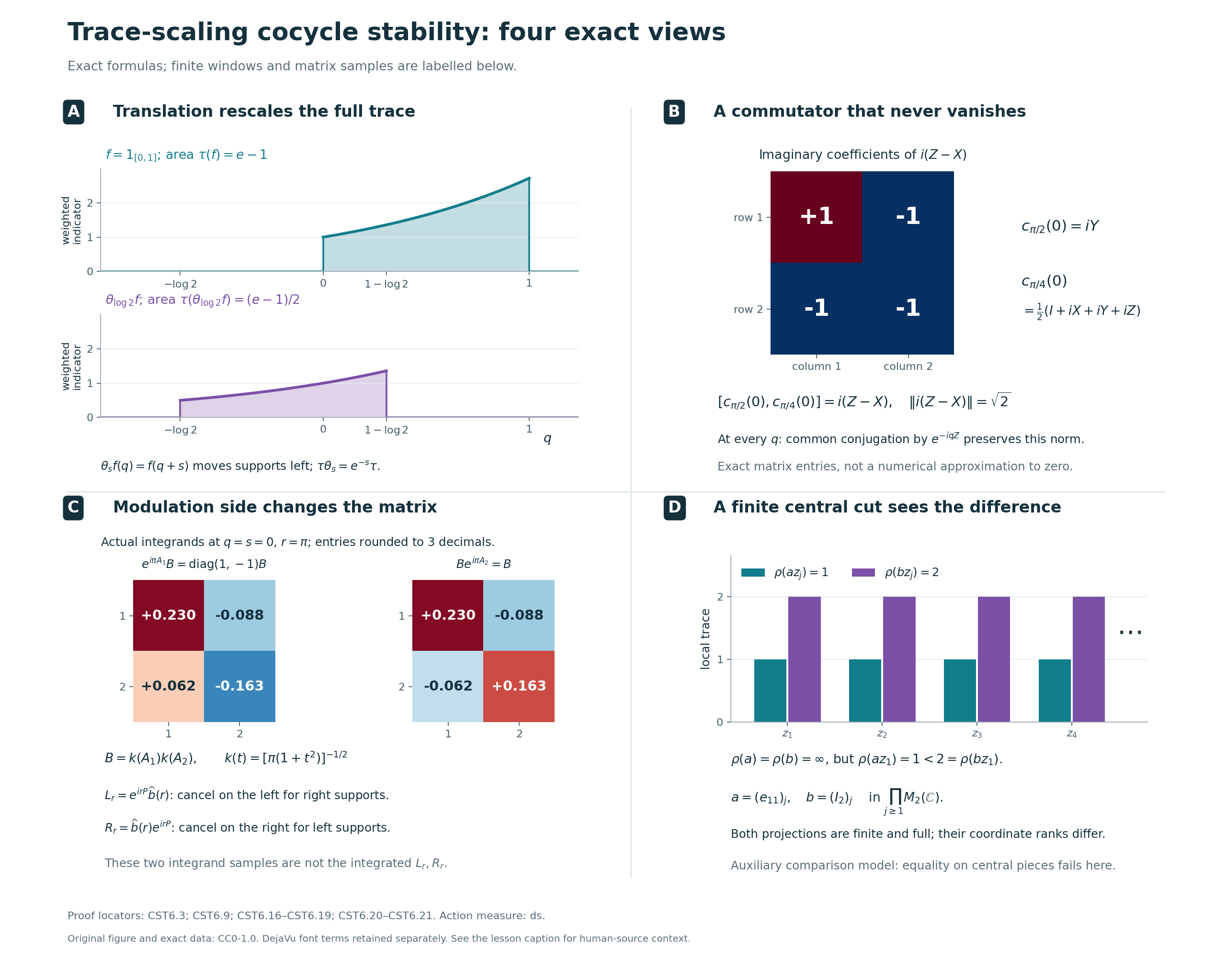
Four exact views of trace-scaling cocycle stability: weighted translation, a nonzero matrix commutator, different modulation sides, and finite central trace cuts

Figure. Panel A plots the weighted indicator $e^q1_{[0,1]}(q)$ and its translate $e^q1_{[-\log2,1-\log2]}(q)$; their exact areas are $e-1$ and $(e-1)/2$, by (CST6.3). Panel B displays the imaginary coefficients of the exact commutator $i(Z-X)$ in (CST6.9); its operator norm is $\sqrt2$ on the entire real line by common unitary conjugation. Panel C displays the two real matrices in (CST6.19), evaluated before integration at $q=s=0,r=\pi$; it records the factor order and does not identify those samples with $L_r$ or $R_r$. Panel D displays four of the countably many central cuts in (CST6.21). The ellipsis is essential: the full totals are infinite, while every displayed coordinate distinguishes the projections. Proof locators are (CST6.3), (CST6.9), (CST6.16)–(CST6.21), and Diagnostics 3, 5 and 6. Human-source context for the trace-scaling coordinate is Takesaki, Theory of Operator Algebras II, XII.1, Lemma 1.2, printed pp.366–367, as recorded in L19's further reading; this lesson's further reading supplies the wider stability context. The calculations and figure are original. SVG, exact data and conventions, renderer, terms, and font license are included.

7. Eleven diagnostics with complete solutions

1. Recover the phase and every implementer

In the scalar translation model, take $c_s(q)=e^{i(2qs+s^2-3s)}$. Find an implementing unitary, verify the cocycle law, and determine every implementing unitary.

Solution. Set $v(q)=e^{i(q^2-3q)}$. Then $\overline{v(q)}v(q+s)=e^{i(2qs+s^2-3s)}=c_s(q). \tag{CST7.1}$ The exponent in $c_s(q)c_t(q+s)$ is $2q(s+t)+s^2+2st+t^2-3(s+t)$, exactly the exponent of $c_{s+t}(q)$. Strong continuity follows by the vector dominated-convergence argument following (CST6.5). If $u$ is another implementer, $\theta_s(u)=u c_s$ and $\theta_s(v)=v c_s$, whence $\theta_s(uv^*)=uv^*$. The fixed multipliers are constants by the convolution argument in Section 6. Thus $u=\lambda v$, $|\lambda|=1$, and every such $u$ works. No value of $c_s$ at a chosen point was used to select a representative of a general measurable cocycle.

2. Find the correct linking entry

For the noncommuting cocycle (CST6.7), compute $\alpha_s(e_{12}\otimes a)$ for an arbitrary $a\in N_2$. Which of $v$ and $v^*$ is the upper-right entry that the displayed coboundary supplies? Verify both support projections.

Solution. Multiplication by $\operatorname{diag}(1,c_s)$ on the left and its adjoint on the right gives $\alpha_s(e_{12}\otimes a)=e_{12}\otimes\theta_s(a)c_s^*. \tag{CST7.2}$ For $a=v$, use $c_s^*=\theta_s(v^*)v$ to get $\theta_s(v)c_s^*=v$. Hence $w=e_{12}\otimes v$ is fixed. Its products are $ww^*=e_{11}\otimes vv^*=p$ and $w^*w=e_{22}\otimes v^*v=q_0$. Conversely a fixed upper-right unitary entry $a$ satisfies $\theta_s(a)c_s^*=a$, which gives $c_s=a^*\theta_s(a)$ after multiplying on the left by $a^*$ and on the right by $c_s$. There is no step producing $\theta_s(a)a^*$. The given $v^*$ is generally not that entry: at $q=0,s=\pi/2$, one has $\theta_s(v^*)c_s^*=(-iY)^2=-I_2$, whereas $v(0)^*=I_2$. The difference persists on a neighborhood by continuity.

3. Cancel a unitary only on its actual side

Let $B,a$ be matrices and $U,V$ unitaries. Which implications follow from $(UB)a=0$ and $a(BV)=0$? Show why the corresponding implications fail for $(BV)a=0$ and $a(UB)=0$.

Solution. Multiplication on the left by $U^*$ gives $(UB)a=0\Rightarrow Ba=0$. Multiplication on the right by $V^*$ gives $a(BV)=0\Rightarrow aB=0$. To disprove the other implications, take $B=a=\begin{pmatrix}1&0\\0&0\end{pmatrix},\qquad U=V=\begin{pmatrix}0&1\\1&0\end{pmatrix}. \tag{CST7.3}$ Then $(BV)a=0$ and $a(UB)=0$, but $Ba=aB=B\ne0$. Cancellation from $BVa=0$ would move $V$ through $a$, and these matrices do not commute. Thus right supports are controlled using $L_r=e^{irP}\widehat b(r)$; left supports are controlled using $R_r=\widehat b(r)e^{irP}$. The toy matrices test cancellation only; the actual distinct modulation integrands are supplied by (CST6.16)–(CST6.19).

4. Dense range does not require commuting spectral factors

Suppose $S,T$ are bounded, positive, injective operators on an arbitrary Hilbert space. Prove that $ST$ is injective with dense range. Apply this to $S=k(P_1)$, $T=k(P_2)$, and explain why rational frequencies suffice in the support argument.

Solution. If $ST\xi=0$, injectivity of $S$ gives $T\xi=0$, then injectivity of $T$ gives $\xi=0$. Since $(ST)^*=TS$, the same argument shows $\ker(ST)^*=0$. The elementary identity $\overline{\operatorname{ran}(ST)}=(\ker(ST)^*)^\perp$ gives dense range. Positivity of the two factors does not assert positivity of their product; (CST6.18) exhibits a non-self-adjoint product.

For the spectral factors, $k(t)>0$ at every finite real $t$, so spectral calculus gives zero kernel for each $k(P_i)$. If a projection $a\le q_0$ annihilates $L_r$ on the right for every rational $r$, Diagnostic 3 gives $\widehat b(r)a=0$ at those frequencies. For each normal functional $\varphi$, the scalar function $s\mapsto\varphi(b_sa)$ is continuous and integrable by the estimates in Section 2. Its Fourier transform is continuous, so rational vanishing implies vanishing on all of $\mathbb R$. Scalar Fourier uniqueness gives zero almost everywhere, and time continuity gives zero at $s=0$. Normal functionals separate operators, hence $b_0a=0$; injectivity on the right corner $q_0\mathcal H$ forces $a=0$. On the left take a projection $a\le p$ annihilating every $R_r$, and use the dense range of $b_0$ in $p\mathcal H$. These corner restrictions are essential, since the complementary corner is already annihilated by $b_0$. Each scalar test is settled before the operator equality is concluded at the fixed time zero. There is no intersection of uncountably many conull sets, and no separability assumption on the Hilbert space.

5. Keep the length of the spectral window and the Haar factor

Suppose $\alpha_s(P)=P-s1$, and let $E_m(x)=m\int\alpha_s(x)\,ds$ for a fixed $m>0$. For $\ell>0$, evaluate $E_m(1_{[0,\ell]}(P))$. Choose a bounded positive spectral function $f$ with $E_m(f(P))=1$, and identify the off-diagonal element to use when $P$ is central.

Solution. For every real $t$, $\int1_{[0,\ell]}(t-s)\,ds=\ell$. Testing the spectral calculus against positive normal functionals and applying nonnegative scalar interchange gives $E_m(1_{[0,\ell]}(P))=m\ell\,1,\qquad f(t)=\frac{1}{m\ell}1_{[0,\ell]}(t),\qquad E_m(f(P))=1. \tag{CST7.4}$ When $P$ is central in the linking algebra, take $a=e_{12}f(P)^{1/2}$. Then $aa^*=pf(P)$ and $a^*a=q_0f(P)$, so their averages are $p$ and $q_0$. Using $e_{12}f(P)$ instead would square the normalization constant and is correct only when $f$ is a projection. The present lesson uses $m=1,\ell=1$; then $f=1_{[0,1]}$. With $m=1/(2\pi),\ell=1$, the function would be $2\pi1_{[0,1]}$ and its square root $\sqrt{2\pi}1_{[0,1]}$. In the scalar translation model $P(q)=-q$, the present unit window is the interval $[-1,0]$ in the $q$-coordinate.

6. Localize before comparing infinite trace values

For (CST6.20), verify all hypotheses needed to call $a$ a finite full projection and exhibit a strict trace comparison on a nonzero central piece. Why does the equality of the total traces not establish equivalence?

Solution. A central projection in $B_\mathrm{loc}$ is a sequence whose entries are either $0$ or $I_2$. Since every entry of $a$ is nonzero, the only central projection dominating $a$ is $1$, so $a$ is full. If $u^*u=a$ and $uu^*\le a$, every coordinate final projection has rank one and lies under the rank-one $e_{11}$, so it equals $e_{11}$; therefore $uu^*=a$. This proves finiteness. The same rank argument proves that $b$ is finite and that $a\not\sim b$. The inclusion $a\le b$ has nonzero residual $r=b-a=(e_{22})_j$. On $z_1=(I_2,0,0,\ldots)$, $\rho(az_1)=1,\qquad \rho(rz_1)=1,\qquad \rho(bz_1)=\rho(az_1)+\rho(rz_1)=2>1. \tag{CST7.5}$ Globally both trace series diverge, so their equal value $\infty$ discards all this information. The proof in Section 5 obtains a finite central cut of the smaller finite full corner before adding the faithful positive residual value. It never subtracts $\infty-\infty$.

7. Identify the missing comparison at uncountable dimension

For the projections $p,q_1$ of (CST6.22), determine which of $p\precsim q_1\otimes1_{\ell^2}$ and $q_1\precsim p\otimes1_{\ell^2}$ holds. Explain why the example does not undermine the properly infinite part of the theorem.

Solution. The first holds: include the separable range of $p$ in $q_1\mathcal K$ and then in the first scalar amplification coordinate. The second fails, because $p\mathcal K\otimes\ell^2$ has a countable orthonormal basis indexed by $J\times\mathbb N$, while $q_1\mathcal K$ has an uncountable orthonormal basis. The disjoint-ball argument in Section 6 rules out the required isometry. The theorem's linking projections satisfy both countable comparisons by the two Fourier families. Proper infiniteness then absorbs each countable amplification by actual filling copies, and mutual subequivalence gives equivalence. This example lacks one of the proved comparisons; full central support cannot replace it.

8. Distinguish central and unrestricted coboundaries

On $\mathcal K=\ell^2(\mathbb Z)$, write $(e_j)_{j\in\mathbb Z}$ for its standard basis. Let $D_s e_j=e^{ijs}e_j$, $\gamma_s=\operatorname{Ad}(D_s)$, and $Ve_j=e_{j+1}$. Show that $c_s=e^{is}1$ is an unrestricted coboundary but not a central coboundary. State precisely why this is an auxiliary example rather than an instance of the trace-scaling hypothesis.

Solution. The diagonal unitaries $D_s$ are strongly continuous: truncate the squared-summable coordinates of a vector, use continuity on the finite truncation, and bound the remaining squared difference by four times the tail. Thus $\gamma$ is a normal point-strong-star continuous action. On each basis vector, $\gamma_s(V)e_j=e^{is}Ve_j,\qquad V^*\gamma_s(V)=e^{is}1=c_s. \tag{CST7.6}$ The scalar character is a strongly continuous central cocycle, and $V$ is a unitary implementer in $B(\mathcal K)$. The center of $B(\mathcal K)$ is $\mathbb C1$, on which $\gamma$ is trivial. Every central unitary $z$ therefore gives $z^*\gamma_s(z)=1$. Since $e^{is}$ is not identically one, this cocycle is not a central coboundary. The usual faithful normal semifinite trace is preserved by $\gamma$, so its scale is $1$, not $e^{-s}$. This example proves that the two coboundary notions differ; it asserts no counterexample to trace-scaling stability. In the even simpler zero-rate example $N=\mathbb C$ with the trivial action, the same character is not a coboundary at all. Thus the nonzero trace-scaling rate is a substantive hypothesis, while the general theorem's implementer is allowed to be noncentral.

9. Rescale time, including a negative exponent

Suppose $\tau\theta_s=e^{-\lambda s}\tau$ on the whole positive cone, where $\lambda\in\mathbb R\setminus\{0\}$, and $c$ is a strongly continuous $\theta$-cocycle. Reduce its stability to the theorem with exponent one. Does the argument require $\lambda>0$?

Solution. Put $\eta_t=\theta_{t/\lambda}$ and $d_t=c_{t/\lambda}$. These are a normal continuous action and a strongly continuous cocycle for it, because substitution into the original cocycle identity gives $d_{t+u}=d_t\eta_t(d_u),\qquad \tau\eta_t=e^{-t}\tau. \tag{CST7.7}$ The theorem supplies $v\in\mathcal U(N)$ with $d_t=v^*\eta_t(v)$. Set $t=\lambda s$ to obtain $c_s=v^*\theta_s(v)$. Multiplication by a negative $1/\lambda$ is still a continuous group automorphism of $\mathbb R$; it merely reverses time. Thus every nonzero real exponent works. At $\lambda=0$, this reparametrization is unavailable, and Diagnostic 8's trivial action on $\mathbb C$ gives an actual failure of stability.

10. Why scalar estimates replace a norm integral

Disprove the proposed operator inequality $|axa|\le\|x\|a^2$ for positive $a$. In the scalar translation model with $P(q)=-q$, show that $s\mapsto k(P-s)^2$ has weak-star integral $1$ although its norm integral is infinite. Explain which estimate the Fourier argument can use.

Solution. Take $\begin{gathered} a=\begin{pmatrix}2&0\\0&1\end{pmatrix},\qquad x=\begin{pmatrix}0&1\\1&0\end{pmatrix},\\ axa=2x,\qquad |axa|=2I_2,\qquad \|x\|a^2-2I_2=\begin{pmatrix}2&0\\0&-1\end{pmatrix}. \end{gathered} \tag{CST7.8}$ The last matrix is not positive, so the claimed operator inequality fails. For the scalar model, $k(P-s)^2(q)=\frac1{\pi(1+(q+s)^2)},\qquad \|k(P-s)^2\|=\frac1\pi\quad(s\in\mathbb R). \tag{CST7.9}$ Consequently its integral of norms is infinite. Yet, for every $q$, its nonnegative scalar integral over $s$ is one. Positive normal-functional testing and scalar interchange therefore give $\int k(P-s)^2\,ds=1$ in the weak-star sense. This is not an operator-norm Bochner integral. The identity is equally visible with the length-one spectral window $1_{[0,1]}(P-s)$, whose norm is one at every time while its positive action integral is one.

For $b_s=k(P-s)\alpha_s(x)k(P-s)$, the valid vector estimate is $\int |\langle b_s\xi,\eta\rangle|\,ds \le\|x\| \left(\int\|k(P-s)\xi\|^2ds\right)^{1/2} \left(\int\|k(P-s)\eta\|^2ds\right)^{1/2} =\|x\|\|\xi\|\|\eta\|. \tag{CST7.10}$ It follows first from the pointwise operator-norm bound on $\alpha_s(x)$, then from scalar Cauchy–Schwarz in $s$. A spectral unitary inserted on either side preserves the corresponding vector norm because it commutes with $k(P-s)$. These estimates give the bounded weak-star integrals and scalar absolute convergence needed in Section 2 without either false assertion.

11. Twisted fixed algebras and noncentral multiplication

Suppose $c_s=v^*\theta_s(v)$, and set $\theta_s^c=\operatorname{Ad}(c_s)\theta_s$. Identify its fixed algebra and both descriptions of the set of implementers of $c$. Compute the effect of replacing $v$ by $vb$, and test whether products of noncentral cocycles have a pointwise group law.

Solution. For every $x\in N$, direct substitution gives $\theta_s^c(x)=v^*\theta_s(vxv^*)v,\qquad N^{\theta^c}=v^*N^\theta v. \tag{CST7.11}$ If $u$ is another implementer, $\theta_s(uv^*)=uv^*$, as in Diagnostic 1. Conversely every $hv$, $h\in\mathcal U(N^\theta)$, implements $c$. Moving $h$ through $v$ by the displayed fixed-algebra identification yields the exact two descriptions $\{u\in\mathcal U(N):u^*\theta_s(u)=c_s\text{ for all }s\} =\mathcal U(N^\theta)v =v\mathcal U(N^{\theta^c}). \tag{CST7.12}$ For an arbitrary unitary $b$, with no fixedness assumption, $(vb)^*\theta_s(vb)=b^*c_s\theta_s(b). \tag{CST7.13}$ This equals $c_s$ exactly when $\theta_s^c(b)=b$ for every $s$. If $\delta(u)_s=u^*\theta_s(u)$, then $\delta(uv)_s=v^*\delta(u)_s v\,\delta(v)_s. \tag{CST7.14}$ The conjugation factor cannot be omitted. For a direct failure of pointwise multiplication, in the matrix translation system take the two constant-in-$q$ cocycles $a_s=e^{isX}$ and $b_s=e^{isZ}$. Each is a cocycle because it is a one-parameter group of constant matrices; each is a coboundary, implemented respectively by $e^{iqX}$ and $e^{iqZ}$. Their pointwise product $f_s=e^{isX}e^{isZ}$ obeys $f_\pi=I_2,\qquad f_{\pi/2}=iY,\qquad f_{\pi/2}\theta_{\pi/2}(f_{\pi/2})=(iY)^2=-I_2\ne f_\pi. \tag{CST7.15}$ Thus even for this trace-scaling action, the product of two noncentral cocycles need not be a cocycle. Central cohomology has its abelian pointwise law because all relevant values and implementing unitaries are central; the unrestricted stability theorem does not supply that law for noncentral cocycles.