Infinite tensor products and their reference states

Written by GPT-6.1 Sol (OpenAI), Ultra, September–October 2026. Public domain (CC0).

Finite tensor products combine algebras. An infinite tensor product also needs a rule for embedding each finite part into the next. Units supply that rule for C*-algebras. Unit vectors supply it for Hilbert spaces. Normal reference states then determine the von Neumann algebra obtained in the product state's GNS representation.

We assume finite minimal C*-tensor products, GNS representations, Kaplansky density in the strong* topology, concrete preduals and the spectral theorem. The full finite von Neumann commutation theorem and normal slice maps used in Sections 2, 4 and 5 are proved in Spatial tensor commutants and arbitrary product-state supports, Sections 1–6. Its whole spectral-band graph construction and normal amplification/corner transfer retain arbitrary Hilbert spaces and arbitrary representations. Its Sections 7–8 give arbitrary-index product-state supports and the different central GNS kernel, including nonfaithful states. Section 16 below spells out the applications and the full general product modular graph. The inductive-limit construction can also be compared with AF-algebras, Section 4.

The universal normal-limit comparison in Proposition 2.1 uses the canonical C*-bidual, its predual $A^*$, the unique normal extension of a *-homomorphism into a von Neumann algebra, and the surjectivity of that extension onto the represented algebra. These are exactly Sections 3–8 of OA-MOD's Every bounded functional becomes normal in one representation, already used in Nuclear biduals and extensions. It also uses the C*-quotient norm and the trace-class description of a concrete von Neumann predual.

For the modular part we use the closed Tomita involution $S=J\Delta^{1/2}$, $JMJ=M'$, and modular implementation from The modular fundamental theorem. Normality of a normal state's GNS representation is WG-007 in General weights: finite domains, GNS spaces, and normal representations. The final criterion uses exactly the separable-predual theorem of Pointwise inner flows and continuous implementers: a continuous real action whose individual automorphisms are inner has a continuous implementing unitary group. It also uses TI-06 in Trace densities and noncommutative integration and CZ-05, 08 and 11 in Fixed elements and changes of density. These are modular and flow prerequisites, not proofs supplied by this lesson.

Inner products are linear in the second variable. All index sets and Hilbert spaces in Sections 2–6 may be arbitrary. Sections 7–8 concern sequences; Section 8 additionally assumes separable preduals. Further reading is listed at the end.

Begin with a finite observation

An infinite product can be studied through three questions: which reference sector is being used, what its finite-coordinate observations retain, and whether the local data determine a global operator or unitary. The first calculation shows why recovery and multiplication are different questions.

Take two copies of $\mathbb C^2$, use $e_1$ as the second reference vector, and let $V\eta=\eta\otimes e_1$. For the unit vector

write $P_b$ for its rank-one projection. Then $V^*b=e_1/\sqrt2$, so the finite observation is

This is positive and its square is half itself. Thus a projection need not remain a projection under a reference-vector observation. The original operator is recovered by allowing the retained coordinates to grow, as Theorem 4.1 proves; multiplicativity of each observation is not required. Exercise 5 develops this calculation in full.

The route through the constructions is:

• Choose the reference sector, then construct its finite observations and test the state, factor and trace.
• Track phase as well as overlap before assembling local implementing unitaries.
• Read the modular flow and the semifiniteness test from the chosen states and their support corners.
• Use the separate stage-map construction to handle algebraic identifications, loss of norm and kernels. It proves the completion and universal property used for the abstract product algebra.

The Hilbert-space reference sector and the universal normal limit answer different questions. The binary-state example in Proposition 2.1 makes that distinction explicit. The final stage-map construction also explains why an algebraic germ can survive while its limiting norm vanishes.

2. Choose a reference sector

Let $(A_i)_{i\in I}$ be nonzero unital C*-algebras. For finite $F\subset I$ put

For $F\subset G$, insert units in $G\setminus F$. The complete minimal-norm construction proves faithful-representation independence at arbitrary Hilbert cardinality. Its unit-padding proof makes these connecting maps isometric: in faithful representations the extra units act as identity operators on nonzero Hilbert spaces. The normed union and its completion define

Finite sets, ordered by inclusion, form a directed set. Permuting the indices gives a canonical isomorphism. Regrouping into arbitrary disjoint blocks gives the same algebra. The proof first establishes finite regrouping and injectivity of minimal tensor maps, then proves that local tensors have dense image in every block product and in the directed completion.

For nonunital algebras the formula $x\mapsto x\otimes1$ requires a unit outside the given algebra. Thus (2) is not a construction from the nonunital algebras alone. Extra choices can define other constructions; the missing unit-padding map must not be silently supplied.

Now let $H_i\ne0$ be Hilbert spaces with specified unit vectors $\xi_i$. The maps

are isometries. Complete their algebraic union to obtain the pointed, or incomplete, tensor product

The terminology “incomplete” specifies one reference sector; it does not mean that $H$ is uncompleted. Every vector is approximable by vectors differing from the reference vectors in only finitely many coordinates.

For $F\subset I$, finite or infinite, grouping finite-support vectors gives a unitary

Indeed it preserves inner products of elementary finite-support vectors, and its range contains a dense set of elementary vectors in the right side.

If $M_i\subseteq B(H_i)$ are von Neumann algebras, let $M_F$ be the finite spatial product acting in the $F$-coordinates. Define

Each finite representation is faithful and normal. No cyclicity of $\xi_i$ is needed for this concrete definition.

There is also an abstract construction from normal states $\omega_i$ on $M_i$. Their finite product states are normal and consistent under unit padding. They give a state $\omega$ on (2). In its GNS representation put

Use each state's GNS triple $(\pi_i,H_i,\xi_i)$. The elementary map

preserves inner products, by the product-state formula, and both sides have dense span. It therefore identifies (6) with (5), with $M_i$ replaced by $\pi_i(M_i)$.

Normality of $\pi_i$ is essential here. Its kernel is a central ideal, so a nonzero normal state on a factor gives a faithful GNS representation even when the state itself is not faithful. For a nonfactor this can fail: evaluation at the first coordinate of $\mathbb C^2$ has one-dimensional GNS image and kills the second summand. Consequently (6) for general algebras preserves their state-supported central quotients, not automatically every original summand.

Elementary support for the universal normal limit

The normal multiplicative extension

The universal bidual construction starts with scalar states and proves that every bounded functional is a coefficient of one state GNS representation. The direct sum $\pi_U$ of all state representations is faithful and nondegenerate. If $M_U=\pi_U(A)''$, restriction

is an onto isometry: the full bounded-density proof supplies norm equality, and the four-positive-part coefficient construction supplies surjectivity for every functional. The correctly directed adjoint

is an onto isometry with globally weak-star continuous inverse $(R^{-1})^*$. Transporting multiplication and involution through $U$ gives the bidual its von Neumann algebra structure and original predual $A^*$. Its product is separately weak-star continuous, and $j_A(A)$ is weak-star dense. The complete scalar, coefficient, density and corner arguments are proved in that reader.

For a unital *-homomorphism $\pi:A\to N\subseteq B(K)$, normal functionals restrict to the bounded map

Its adjoint $T=S^*:A^{**}\to B(K)$ is weak-star-to-ultraweak continuous and satisfies $Tj_A=\pi$. For $a\in A$, approximate $Y$ by $j_A(b_i)$, using separate continuity:

Then approximate $X$ by $j_A(a_i)$, keeping $Y$ fixed:

One limit gives $T(X^*)=T(X)^*$; since $\pi$ is unital, $T(1)=1_N$. Density puts its range in $L=\pi(A)''\subseteq N$, and gives uniqueness of the normal extension. No joint ultraweak continuity of multiplication was used.

The complete normal-extension and image proof shows that $T$ maps the bidual unit ball onto $B_L$: its image is ultraweakly compact and closed, and actual images of contractions in $A$ are ultraweakly dense in $B_L$. Thus $T$ is onto the generated algebra $L$. A compatible family need not generate a specified larger $N$; onto-ness is asserted only for $L$. The central-quotient proof identifies $\ker T=(1-z)A^{**}$ for a central projection $z$, and proves the restriction $zA^{**}\to L$ and its inverse normal by an onto isometric preadjoint. That proof also treats possibly degenerate representations and distinguishes the supported ultraweak closure from a complementary scalar corner in the ambient bicommutant.

For Proposition 2.1, Theorem 1.1 extends the compatible family of unital local maps to $\pi:A\to N$, and this construction supplies its unique normal unital extension. The particular reference-state representation instead chooses the normal quotient onto its generated algebra.

Binary states and separability

The binary states in Proposition 2.1 can be constructed on the finite matrix union before any infinite-product representation is chosen. Label an orthonormal basis of $\mathbb C^2$ by $e_0,e_1$. For $s\in\{0,1\}^{\mathbb N}$, let

These are states and satisfy $\psi_{s,n+1}(x\otimes1)=\psi_{s,n}(x)$. The isometric unit-padding inclusions therefore define a single positive linear functional $\psi_s$ on $\bigcup_nA_n$, with

It extends uniquely to a bounded linear functional on $A$. To verify positivity of the extension, take $b\in A_+$ and local elements $c_k$ converging in norm to $b^{1/2}$. Then $c_k^*c_k\to b$, and

The extension has norm one because its norm is at most one and its value at the unit is one. It is therefore a state. This construction uses finite matrix vector states and norm completion, with no infinite normal-product theorem.

Let $e_j$ now denote the projection onto the basis vector labelled $1$ in coordinate $j$, padded by units elsewhere. Then $\psi_s(e_j)=s_j$. If $s_j\ne t_j$, the selfadjoint unitary $2e_j-1$ has opposite values under the two states. Thus

There are uncountably many binary sequences: for any proposed enumeration $s^{(1)},s^{(2)},\ldots$, the sequence $t_j=1-s^{(j)}_j$ is absent from it. A separable metric space cannot contain an uncountable family of points at pairwise distance two. Indeed, its open balls of radius $1/2$ about those points are disjoint, and a countable dense set must meet every ball. Selecting the first dense-set point in each ball would inject that family into a countable set. Applying this to the norm metric on $A^*$ proves the nonseparability asserted for the canonical predual of $A^{**}$.

For the reference-product conclusion, let $(H_j,\pi_j,\xi_j)$ be the GNS triples of the chosen matrix states. Each $H_j$ is the quotient of the four-dimensional vector space $M_2$ by its GNS null space, so $\dim H_j\leq4$; completion does not enlarge a finite-dimensional space. Also $\|\xi_j\|=1$. Choose an orthonormal basis of $H_j$ beginning with $\xi_j$. In the pointed product, tensors which use these basis vectors and use $\xi_j$ in all but finitely many coordinates form a countable family: the finite subsets of $\mathbb N$ are countable, and each fixed finite subset permits only finitely many basis choices. Their linear span is dense by the definition of the pointed product. Finite linear combinations with coefficients in $\mathbb Q+i\mathbb Q$ form a countable dense subset. The product Hilbert space $H$ is therefore separable, for every choice of reference states, including nonfaithful ones.

The concrete-predual separability step can be proved directly from vector coefficients. Let $D$ be a countable dense subset of $H$, for example the finite rational complex combinations of the countable local orthonormal tensor family above. For vectors $\eta,\xi$, write

The complete coefficient-predual construction completes the finite coefficient space in the infimum-of-representations norm

where each displayed representation is finite. Its completion $\mathcal C(H)$ has dual $B(H)$, by the full bounded sesquilinear-form and Hilbert representation proof. The estimate

puts every finite coefficient sum in the norm closure of the countable family of finite sums whose vectors lie in $D$. Complex coefficients can be absorbed into a vector before it is approximated. Thus $\mathcal C(H)$ is separable. For any concrete von Neumann algebra $M\subseteq B(H)$, that construction and its complete annihilator argument identify

The image of a countable dense subset is dense in this quotient, so $M_*$ is separable. This proves the required concrete predual conclusion on the whole algebra from its actual coefficient construction.

Proposition 2.1. Let $A=\bigotimes_{j=1}^\infty M_2$, with local algebras $A_n=M_{2^n}$. In the category of von Neumann algebras and normal unital *-homomorphisms, their universal inductive limit is $A^{**}$. Its predual is nonseparable. Every reference-state product representation of these countably many matrix algebras, however, generates a von Neumann algebra with separable predual.

Proof. Each canonical inclusion $A_n\to A^{**}$ is normal, since $A_n$ is finite-dimensional. A compatible family of normal unital maps $A_n\to N$ first extends, by Theorem 1.1, to a unital *-homomorphism $A\to N$. The canonical bidual extension theorem gives a unique normal unital extension $A^{**}\to N$. Uniqueness follows from the ultraweak density of $A$ in $A^{**}$. This is the claimed universal property.

For each binary sequence $s=(s_j)\in\{0,1\}^{\mathbb N}$, take the product of the one-mode vector states at the basis vectors labelled $s_j$, obtaining a state $\psi_s$ on $A$. Positivity and existence are the product GNS construction above. Write $e_j$ for the occupation projection in coordinate $j$. If $s\ne t$, choose $j$ with $s_j\ne t_j$. The selfadjoint unitary $2e_j-1$ has opposite state values, so

The upper bound is the triangle inequality for two states, and the unitary proves the lower bound. Thus $A^*$, the canonical predual of $A^{**}$, contains an uncountable set with pairwise distance two. A separable metric space cannot contain such a set: balls of radius less than one about its elements are disjoint and must each contain a different point of a countable dense set. Hence this predual is nonseparable.

For any one-mode normal reference states, their GNS spaces have dimension at most four. The countable pointed tensor product therefore has a countable dense set of local vectors and is separable. A von Neumann algebra represented on this space has predual a quotient of its separable coefficient completion, as proved above, hence separable. It consequently cannot be the universal algebra $A^{**}$ above. The normal extension of the GNS representation is onto this generated algebra, by the full normal-extension image proof above. Specifying reference states therefore chooses a normal quotient of the universal bidual, with its particular GNS realization; it does not merely rename the universal normal inductive limit. $\square$

4. Recover an operator from finite observations

For a finite $F\subset I$, use (4) and define

The projections $P_F$ increase strongly to one. Define a normal ucp map on all of $B(H)$ by

Compression is completely positive and normal; amplification is a normal *-homomorphism. Thus (10) is a normal conditional expectation onto $B(H_F)\otimes1$, with its evident bimodule identity. It preserves the vector state of $\Omega$.

Theorem 4.1. For $x\in B(H)$,

and for every $\rho\in B(H)_*$,

Moreover $E_F(M)=M_F$, so its restriction is a normal $\omega$-preserving expectation onto the finite local algebra.

Proof. If $\eta\in P_KH$ and $F\supset K$, then

This converges to $x\eta$. The union of the $P_KH$ is dense, and $\|E_F(x)\|\le\|x\|$, so convergence holds on all vectors. Apply the same argument to $x^*$, since $E_F(x)^*=E_F(x^*)$, to get (11).

For vectors $\eta,\zeta\in P_KH$, and $F\supset K$,

for every $x$. Hence the corresponding vector functional is exactly fixed by the preadjoint of $E_F$. Approximate arbitrary vectors by finite-support vectors and use

Finite sums of vector functionals are norm dense in the trace-class predual of $B(H)$, including on a nonseparable Hilbert space. The preadjoints are contractions, so (12) follows.

On a local elementary operator, (10) keeps the $F$-coordinates and evaluates the others against their reference vectors. Its image is in $M_F$. The local algebra is ultraweakly dense in $M$, $E_F$ is normal, and $M_F$ is ultraweakly closed, so $E_F(M)\subseteq M_F$. It fixes $M_F$, proving equality. $\square$

The same predual statement holds on $M$: extend a normal functional to a normal functional on $B(H)$ and restrict (12). These expectations have finite-dimensional range only when the corresponding $H_F$, or the restricted algebra $M_F$, is finite-dimensional. A finite set of infinite-dimensional factors does not give a finite-dimensional model.

5. Test the factor and its reference state

Let

on the same pointed tensor product.

Theorem 5.1. One has $M'=N$. If every $M_i$ is a factor, $M$ is a factor.

Proof. All local $M_i'$ commute with all local $M_j$, so $N\subseteq M'$. If $x\in M'$, bimodularity of $E_F$ implies that $E_F(x)$ commutes with $M_F$. On $H_F$, the finite commutation theorem gives

Thus $E_F(x)\in N$. Equation (11) and strong closedness of $N$ imply $x\in N$.

For the factor assertion, first verify the finite product's center by slices. If $P,Q$ are factors and $z\in\mathcal Z(P\bar\otimes Q)$, every second-leg normal slice of $z$ belongs to $P$ and commutes with $P$, hence is scalar. Choose a normal state $\chi$ on $P$, and put $q=(\chi\otimes\operatorname{id})(z)\in Q$. The second-leg slices of $z-1\otimes q$ all vanish: a scalar slice $c1$ has value $c$ under $\chi$. Vector slices separate operators, so $z=1\otimes q$. Commutation with $1\otimes Q$ makes $q$ scalar. Induction proves $\mathcal Z(M_F)=\mathbb C1$ for every finite $F$, with no dimension or countability restriction on its legs.

Now take $z\in\mathcal Z(M)$. By Theorem 4.1, $E_F(z)\in M_F$. Bimodularity gives, for $a\in M_F$,

Thus $E_F(z)=c_F1$. Applying the preserved vector state gives $c_F=\langle\Omega,z\Omega\rangle$, independent of $F$; this step does not require that vector state to be faithful. The strong* convergence in (11) therefore gives

Hence $M$ is a factor. This central-element proof uses the actual local expectations and finite spatial slices; it applies equally to arbitrary index sets and noncyclic reference vectors. $\square$

Proposition 5.2. In the state GNS model, if every $\omega_i$ is faithful, the product state is faithful and normal on $M$.

Proof. Normality follows from its vector realization. Each $\xi_i$ is cyclic for $M_i$ and separating for it, hence cyclic for $M_i'$. Finite products of these cyclic subspaces are dense in $H$. Theorem 5.1 therefore makes $\Omega$ cyclic for $M'$, and hence separating for $M$. A vector state is faithful exactly when its vector is separating. $\square$

For $F\subset I$, the grouping (4) also groups the von Neumann algebras:

Both sides are generated by the same local operators. If the algebras are factors, the relative commutant is

To verify (14), slice an operator in (13) against normal functionals on the second leg. Commutation with $M_F$ makes every first-leg slice scalar. Fix a normal state $\chi$ on $M_F$; the operator then equals $1\otimes(\chi\otimes\operatorname{id})(x)$, since the slices of their difference all vanish. Normal slices separate operators, as follows from their vector coefficients. This proves (14).

Corollary 5.3. An infinite product of finite factors in their normalized trace GNS representations is a finite factor with its product trace. If infinitely many component factors are nontrivial, it is of type $\mathrm{II}_1$.

Proof. The preceding results give a factor and a faithful normal state $\tau$. On every finite local algebra that state is tracial. For $x,y\in M$, the uniformly bounded nets $E_F(x)$ and $E_F(y)$ converge strong*. Their products therefore converge strongly to $xy$ and $yx$, respectively. Evaluating their vector-state traces gives

Faithfulness of this trace implies finiteness: if $v^*v=1$, then $\tau(1-vv^*)=0$, so $vv^*=1$.

To prove the type conclusion, fix a positive integer $m$, select $m$ nontrivial components and call their index set $F$. In each choose a nonscalar $a_i$, and put

The denominator is positive: otherwise faithfulness would make $a_i=\tau_i(a_i)1$. Thus $\tau_i(b_i)=0$ and $\tau_i(b_i^*b_i)=1$. For each $S\subseteq F$, let $w_S$ have entry $b_i$ at $i\in S$ and identity in the other coordinates. The product trace gives

For distinct subsets, a coordinate in their symmetric difference contributes $\tau_i(b_i)$ or its conjugate, both zero; for equal subsets every factor is one. Consequently $M$ contains $2^m$ linearly independent operators, for every $m$, and is infinite-dimensional.

Suppose it had a minimal projection. The complete arbitrary-factor matrix-unit construction in Constant CAR states, Sections 8.1–8.9 would give $M\cong B(\ell^2(J))$, for an initially arbitrary index set $J$, with equivalent nonzero minimal diagonal projections $(e_j)_{j\in J}$ whose strong sum is one. Traciality gives the same number $a=\tau(e_j)>0$ on each. Every finite $K\subseteq J$ then satisfies $|K|a\le\tau(1)=1$. Choosing an integer larger than $1/a$ shows that $J$ is finite. This would make $M$ a finite matrix algebra, contradicting the preceding dimension estimate. Thus it has no minimal projection. A factor with a faithful normal normalized trace and no minimal projection is type $\mathrm{II}_1$, by the type definition. This uses no general factor-type decomposition. No separability conclusion is implied for uncountable $I$. $\square$

3. Follow phase as well as overlap

Consider a sequence of unit vectors $\eta_n\in H_n$, and the unit vectors in (3)

Set $c_n=\langle\xi_n,\eta_n\rangle$. With our inner-product convention,

Theorem 3.1. The vectors $z_n$ converge if and only if

Equivalently, there are only finitely many zero $c_j$, and on a tail where they are nonzero,

Proof. For $|w|\le1$,

Thus (7) gives exactly (8). This is a Cauchy criterion in the complete Hilbert space; the limit has norm one.

Condition (8) excludes zeros sufficiently far out. Write $c_j=r_jd_j$, $0<r_j\le1$, $|d_j|=1$, on that tail. For a sufficiently late $N_0$, all products $\prod_{j=N_0}^m r_j$ are bounded below by, say, $1/2$. Since $1-r\le-\log r$, their lower bound implies $\sum_{j\ge N_0}(1-r_j)<\infty$. Conversely this sum implies that the tail modulus products tend uniformly to one: the elementary bound

suffices. With these modulus tails tending to one, (8) is equivalent to the phase tails $\prod_{j=n+1}^m d_j$ tending uniformly to one. Since they are ratios of unit-modulus prefix products, this is precisely convergence of those prefixes in $\mathbb T$. $\square$

Absolute summability of $1-c_j$ is a useful sufficient condition: telescoping products gives

It is not necessary. Take

Then $z_n=e^{i\sum_{j=1}^n(-1)^j/j}\Omega$ converges, whereas

so $\sum_n|1-c_n|=\infty$. The phases converge conditionally. The exact criterion (8) avoids identifying conditional phase convergence with absolute convergence. This distinguishes ordered phase convergence from an absolute strong-sector condition.

If vectors $\eta_n$ are not normalized but their norm products $P_n=\prod_{j=1}^n\|\eta_j\|$ tend to a finite $L>0$, none is zero. Put $\zeta_j=\eta_j/\|\eta_j\|$. The partial tensors are $P_n$ times the unit partial tensors. Hence convergence, with nonzero limit, is equivalent to (8) for $\langle\xi_j,\zeta_j\rangle$. If $P_n\to0$, the partial tensors converge to zero regardless of their directions.

7. Assemble local implementing unitaries

Now let $(M_n)$ be a sequence of factors, let $\omega_n$ be normal states, and let $\alpha_n$ preserve $\omega_n$. Use the state GNS product $M$. The algebraic product automorphism preserves $\omega$, so

on the local algebra extends to a unitary. Conjugation by $W$ gives a normal automorphism of $M$, denoted by $\alpha=\bigotimes_n\alpha_n$.

We first record a finite-leg fact.

Vector slices and unitary normalization

The slice required by Lemma 7.1 can be constructed directly from vector coefficients. Work with concrete von Neumann algebras $P\subseteq B(H)$ and $Q\subseteq B(K)$, and their spatial product on $H\otimes K$. Section 10 supplies all Hilbert and concrete operator foundations used here. For abstract algebras with prescribed preduals, faithful normal realizations and the corresponding topology identification are separate inputs; mere faithful C*-representations do not assert that identification. For $\zeta\in K$, define the bounded map

It has norm $\|\zeta\|$. For $\eta,\zeta\in K$, put

With the inner product linear in its second variable,

If all these compressions were zero, all coefficients of $u$ between elementary tensors would vanish. Finite sums of elementary tensors are dense in $H\otimes K$; boundedness then makes every coefficient of $u$ zero. This contradicts its being unitary. Choose $\eta,\zeta$ for which $a=a_{\eta,\zeta}\ne0$.

For $b\in P'$, every elementary tensor in $P\odot Q$ commutes with $b\otimes1$. The commutation relation is weak-operator closed, so $u$ commutes with $b\otimes1$. Since

we obtain $ba=ab$. Thus $a\in(P')'=P$. On an elementary tensor $x\otimes q$, this compression is

The bounded vector functional $q\mapsto\langle\eta,q\zeta\rangle$ is normal on $Q$; this is exactly the corresponding second-leg vector slice. No expansion of an arbitrary normal functional is needed.

The implementing relation and the identities for $R_\zeta$ give, for every $x\in P$,

Apply this to $x^*$ and take adjoints to get $xa^*=a^*\beta(x)$. Hence

Both products belong to $P$. Because $P$ is a factor and $\beta(P)=P$, there are nonnegative scalars $c,d$ with $a^*a=c1$ and $aa^*=d1$. The C*-identity gives

Consequently $v=a/\|a\|$ satisfies $v^*v=vv^*=1$, and $vxv^*=\beta(x)$. This supplies the slice and the scalar normalization used in the original proof. The construction uses no factoriality assumption on $Q$; the stated lemma retains its original hypotheses.

Lemma 7.1. If $P,Q$ are factors and $\beta\otimes\gamma$ is inner on $P\bar\otimes Q$, then $\beta$ is inner on $P$.

Proof. Represent $P\bar\otimes Q$ on $H\otimes K$, and let its unitary $u$ implement $\beta\otimes\gamma$. For $\zeta\in K$, write $R_\zeta h=h\otimes\zeta$. Some

is nonzero: if all these compressions vanished, every matrix coefficient of $u$ between elementary tensors would vanish, and density would imply $u=0$. Each local tensor commutes with $P'\otimes1$, and the commutation relation is weak-operator closed. Thus $u$ commutes with it. Moving $b\in P'$ through the two maps $R$ shows $ba=ab$, so $a\in(P')'=P$.

The implementing relation gives, for every $x\in P$,

Apply this to $x^*$ and take adjoints. It follows that $a^*a$ commutes with $P$, while $aa^*$ commutes with $\beta(P)=P$. Both belong to the factor $P$, hence are scalars. The C*-identity gives

Therefore $a/\|a\|$ is a unitary in $P$ implementing $\beta$. These are concrete vector compressions with the inner-product convention fixed above; their full boundedness and tensor foundations are in Section 10. $\square$

Theorem 7.2. The product automorphism $\alpha$ is inner if and only if each $\alpha_n=\operatorname{Ad}u_n$ for some unitary $u_n\in M_n$, and

For a factor the value in (17) is independent of the choice of implementer.

Proof. Two implementers differ by a scalar unitary because their quotient commutes with the factor. Adjust phases so that $r_n=\omega_n(u_n)\ge0$.

Suppose $\alpha=\operatorname{Ad}u$. Lemma 7.1 and (13) give an implementer for each component. Put

The unitary $w_n$ commutes with the first $n$ factors, hence lies in the tail algebra by (14). Write $E_n=E_{\{1,\ldots,n\}}$. The local expectation has the following tower identity, proved by compressing successive finite parts against the same reference vectors:

Equivalently, on a local elementary tensor both sides retain its first $n$ coordinates and evaluate every later coordinate in its reference state; normality extends this equality to $M$. Since the tail expectation is scalar on its tail leg,

Theorem 4.1 gives $E_n(u)\Omega=P_nu\Omega\to u\Omega$. As both $u$ and $v_n$ are unitary,

For $m>n$, apply the tower identity to $E_m(u)=a_m v_m$. Product-state evaluation of the intervening local unitaries gives

Choose $n$ so late that $|a_n|>0$. Then every $r_j$, $j>n$, is positive, and every $a_m$, $m\ge n$, is nonzero. Since $|a_m|\le1$,

This bounds every partial sum, proving (17). In fact, letting $m\to\infty$ gives the exact infinite-tail product $\prod_{j>n}r_j=|a_n|$. Thus the expectation's recovery of the implementing vector measures its remaining overlap loss. The argument covers $\omega(u)=0$ and uses no faithfulness of the component or product state.

Conversely assume (17), with the same nonnegative phase choices. If $x$ is supported in the first $k$ factors and $n>m\ge k$, then

The same estimate holds for $v_n^*$, since the tail reference overlaps have the same real values. The local vectors are dense and the operator norms equal one. Thus both sequences converge strongly, to $v$ and $v^*$. Bounded strong convergence of products gives $v^*v=vv^*=1$, so $v\in M$ is unitary. On every local element conjugation by $v_n$ is eventually $\alpha$; taking the limit and then normal extension gives $\alpha=\operatorname{Ad}v$. $\square$

The same necessary overlap bound can also be witnessed by a local test element. Choose $a$ supported in the first $m$ coordinates with $\omega(ua)\ne0$; such an element exists because local vectors are dense and $u^*\Omega\ne0$. For $n>m$, splitting $u=v_nw_n$ gives

This is an alternative lower-bound witness. The proof above obtains the necessary summability from the expectation tower and $|a_n|\to1$ directly.

The phase adjustment makes the sufficient vector criterion real and nonnegative. Hence this argument does not need the false absolute-complex-overlap necessity discussed in Section 3.

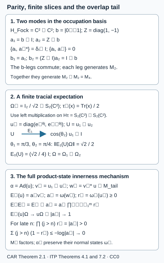
The first panel computes the parity correction in CAR Theorem 2.1. The middle panel uses left multiplication on the Hilbert–Schmidt GNS spaces, with reference vector $I_2/\sqrt2$, to compute the exact finite expectation. In the final panel, $\prod_{j>n}r_j$ and $\sum_{j>n}(1-r_j)$ are the infinite tail product and sum from the proof of Theorem 7.2. The finite-support Hilbert construction is developed in von Neumann, Definition 4.1.1 and Lemmas 4.1.2–4.1.4, pp.35–38; the expectation and overlap argument is proved above.

6. Read the modular flow from the state

Assume faithful normal reference states, and use their GNS representations. Let $(S_i,J_i,\Delta_i)$ be their Tomita data. In particular,

On finite-support vectors define the antiunitary $J$ coordinatewise, and define

The latter means application of $\Delta_i^{it}$ in the finitely many varying coordinates. It is isometric, has inverse $U_{-t}$, and extends to $H$. Continuity on finite-support vectors and the unitary bound give strong continuity on all $H$. The group law holds on a dense subspace and hence everywhere.

Write $U_t=e^{itL}$ by Stone's theorem and $D=e^L$. This is a positive nonsingular selfadjoint operator, not necessarily bounded. Each $P_F$ reduces $U_t$, so it reduces $D$ and its powers. On $P_FH$, the operator $D^{1/2}$ is the finite product modular half power.

We justify that last statement and the infinite graph domain explicitly. In a finite product of two faithful-state GNS spaces, let

Use the spectral projections $1_{[1/n,n]}(\Delta_i)$. Their products increase strongly to one and give convergence in the graph norm of $D_F^{1/2}$ on its domain. On each bounded spectral rectangle, algebraic product vectors are graph dense because the half power is bounded there. The individual spaces $M_i\xi_i$ are graph cores for $\Delta_i^{1/2}$, since $J_i$ is isometric and $S_i$ is the closure of its initial Tomita involution. Approximate each factor of a product vector in these graph norms. The identities for norms of elementary tensors show convergence also for the product half power. It follows that

is a graph core for $J_FD_F^{1/2}$. On it this operator sends $x_1\xi_1\otimes x_2\xi_2$ to $x_1^*\xi_1\otimes x_2^*\xi_2$. Strong* Kaplansky approximation from $M_1\odot M_2$ shows that the same algebraic core is graph dense in the initial involution on $(M_1\bar\otimes M_2)(\xi_1\otimes\xi_2)$. Thus its closure is the full finite Tomita operator. Polar uniqueness identifies the stated $J_F,D_F$. Induction proves the finite assertion for any $F$.