The Riemann hypothesis and its standard equivalents
Written and self-checked by GPT-6.1 Sol (OpenAI) in Codex, Ultra setting, October 2026. Self-check is by the writing AI. Original exposition and calculations are public domain (CC0). The identified adaptation in Sections 6.1–6.5 retains CC BY 4.0.
The Riemann hypothesis says that every nontrivial zero has real part one half. Through the explicit formula, this gives a square-root scale for the error in counting primes. Conversely, a sufficiently small prime-counting error continues the logarithmic derivative into a larger half-plane and excludes zeros there. We prove both directions and the corresponding equivalents involving the Möbius function. We then develop the divisor-sum and fractional-part approximation criteria, connecting the latter to a full Mellin-space proof. Exact lessons supply the positivity criteria and the finite-field theorem. These different formulations also explain what finite numerical evidence can establish.
The functional equation and zero symmetries are proved in Poisson summation, theta, and the functional equation. We use Perron's formula and the explicit formula for prime counting, Theorem 2.2, and the zero-count estimates in Counting the zeros, Theorem 4.1. Partial summation and prime-power comparisons come from Counting primes by elementary means. The bounded-coefficient Perron formula is The prime number theorem with the classical error term, Lemma 3.1. The analytic bridge below uses the fully proved Borel–Carathéodory and strip-interpolation arguments from lessons five and six.
Write $M(x)=\sum_{n\le x}\mu(n)$, $\psi(x)=\sum_{n\le x}\Lambda(n)$ and $\theta(x)=\sum_{p\le x}\log p$. Here $\psi$ never denotes the gamma logarithmic derivative. Set $\tau=|t|+4$. We use $\operatorname{li}(x)=\operatorname{Ei}(\log x)$, rather than the shifted integral $\operatorname{Li}(x)=\int_2^xdu/\log u$.
The integration and complex-analysis tools used in this lesson are proved in Dirichlet series and Euler products, Appendix A, Lemmas A.1–A.4.
1. The zero boundary and prime counting
Theorem 1.1. Suppose $1/2\le\Theta\le1$ and every nontrivial zero satisfies $\beta\le\Theta$. Then $$ \psi(x)-x\ll x^\Theta\log^2x\qquad(x\ge2). \tag{1.1} $$ Conversely, if $0\le\alpha<1$ and, for every $\varepsilon>0$, $$ \psi(x)-x=O_\varepsilon(x^{\alpha+\varepsilon}), \tag{1.2} $$ then every nontrivial zero has $\beta\le\alpha$.
Proof. Set $T=x$ in the sharp explicit formula. The sum of $1/|\rho|$ over $|\gamma|<x$ is $O(\log^2x)$, so its zero contribution is at most $Cx^\Theta\log^2x$. The remaining terms are $O(\log^2x)$ and the half-weight correction at a prime power is $O(\log x)$. They are absorbed in (1.1).
For the converse put $E(u)=\psi(u)-u$. In $\Re s>1$, partial summation gives $$ -\frac{\zeta'}\zeta(s) =s\int_1^\infty\psi(u)u^{-s-1}\,du =\frac{s}{s-1}+s\int_1^\infty E(u)u^{-s-1}\,du. \tag{1.3} $$ Thus the exact pole-subtracted identity is $$ -\frac{\zeta'}\zeta(s)-\frac1{s-1} =1+s\int_1^\infty E(u)u^{-s-1}\,du. \tag{1.4} $$ The constant one is the contribution of the lower endpoint in the integral of $u$.
The right side of (1.4) is holomorphic for $\Re s>\alpha$. On any compact subset choose $\varepsilon>0$ smaller than its distance from that boundary. The majorant $C_\varepsilon u^{\alpha+\varepsilon-\sigma-1}$ is integrable uniformly there; it justifies holomorphy by locally uniform convergence of the truncated integrals. The identity theorem for meromorphic functions extends (1.4) to that half-plane. A zero of order $m$ at $\rho\ne1$ would give a pole of residue $-m$ on its left side, whereas its right side is holomorphic. Hence no zero lies there. $\square$
The hypotheses force $\alpha\ge1/2$ if they hold: the functional equation pairs a zero of real part $\beta$ with one of real part $1-\beta$, and there are nontrivial zeros. We need no assumption that the supremum of the real parts is attained.
2. Von Koch's prime-counting bounds
Theorem 2.1. Under RH, $$ \psi(x)=x+O(\sqrt x\log^2x),\qquad \pi(x)=\operatorname{li}(x)+O(\sqrt x\log x). \tag{2.1} $$ Conversely the second bound implies RH.
Proof. The first bound follows from Theorem 1.1 with $\Theta=1/2$. Since $\psi(x)-\theta(x)\ll\sqrt x$, it gives $\theta(x)=x+O(\sqrt x\log^2x)$. In the exact identity $$ \pi(x)=\frac{\theta(x)}{\log x} +\int_2^x\frac{\theta(u)}{u\log^2u}\,du, $$ the endpoint error is $O(\sqrt x\log x)$ and the error integral is $O(\int_2^x u^{-1/2}du)=O(\sqrt x)$. The main terms equal $\operatorname{Li}(x)+2/\log2$, whose constant difference from $\operatorname{li}(x)$ is absorbed. This proves the second bound.
Conversely, write $\pi(x)=\operatorname{li}(x)+R(x)$, with $R(x)=O(\sqrt x\log x)$. Partial summation gives $$ \theta(x)=\pi(x)\log x-\int_2^x\frac{\pi(u)}u\,du. $$ Replacing $\pi$ by $\operatorname{li}$ yields $x$ plus a fixed constant: the derivative of the resulting expression is one. Its error is $$ R(x)\log x-\int_2^xR(u)u^{-1}du =O(\sqrt x\log^2x), $$ since $\int_2^x u^{-1/2}\log u\,du\ll\sqrt x\log x$. Restoring prime powers gives the same bound for $\psi-x$. Theorem 1.1 excludes zeros with real part greater than $1/2$, and symmetry excludes those with real part less than $1/2$. $\square$
3. A reciprocal bound under RH
The implication from RH to a bound for $M(x)$ needs a growth estimate for $1/\zeta$, as well as nonvanishing. A zero-free half-plane alone does not supply that estimate.
Lemma 3.1 (interpolation of logarithmic powers). Let $a<b$ and $f$ be holomorphic on a neighbourhood of their closed vertical strip. Suppose $f$ grows at most $D\exp(D(1+|t|)^C)$ there and $$ f(a+it)\ll\log(|t|+4),\qquad f(b+it)\ll1. $$ Then $$ f(\sigma+it)\ll(\log(|t|+4))^{(b-\sigma)/(b-a)} \qquad(a\le\sigma\le b). \tag{3.1} $$
Proof. Fix $t_0$, set $T=|t_0|+4$, $L(z)=(b-z)/(b-a)$, and choose $c$ with $a+c\ge1$. Normalize by $$ g(z)=\frac{f(z+it_0)\exp(-L(z)\log\log T)}{z+c}. $$ On the left boundary, $\log(|t_0+y|+4)/\log T\le1+|y|$, while $|a+c+iy|\gg1+|y|$. The modulus of the exponential factor is $1/\log T$ there. On the right boundary its modulus is one, and the denominator is bounded away from zero. Thus both boundary values of $g$ are bounded independently of $t_0$.
Choose $0<k<\pi/(b-a)$ and multiply $g(z)$ by $\exp[-\epsilon\cos(k(z-(a+b)/2))]$. The real part of the cosine is at least $\cos(k(b-a)/2)\cosh(k\Im z)>0$ throughout the strip. This damping makes the horizontal boundaries tend to zero and leaves the vertical bound unchanged. The maximum principle on increasing rectangles, followed by $\epsilon\downarrow0$, bounds $g$ in the strip. At real $z=\sigma$, restoring its normalization proves (3.1). $\square$
Theorem 3.2. Assume RH. For every fixed $\sigma_0>1/2$ and every $\varepsilon>0$, $$ \frac1{\zeta(\sigma+it)}\ll_{\sigma_0,\varepsilon}\tau^\varepsilon \qquad(\sigma\ge\sigma_0). \tag{3.2} $$ The reciprocal has its removable zero at one.
Proof. The function $F(s)=(s-1)\zeta(s)$ is holomorphic and nonzero in $\Re s>1/2$ under RH, including $F(1)=1$. This half-plane is simply connected, so $$ H(s)=\log\frac{F(s)}{s+1} $$ has an analytic branch, normalized by its real value at $s=2$. On the line two it equals the Euler logarithm plus $\log(s-1)-\log(s+1)$, with the usual branches in the right half-plane; both terms are uniformly bounded there. Hence $H(2+it)=O(1)$.
Fix $0<\delta<1/4$. On the disc centred at $2+it$ of radius $3/2-\delta$, the elementary growth bound for zeta gives $\Re H=O_\delta(\log\tau)$. Away from a fixed neighbourhood of one use $$ \Re H(s)=\log|\zeta(s)|+\log\left|\frac{s-1}{s+1}\right|, $$ where the second term is nonpositive for $\Re s>0$. Zeta has polynomial growth on the fixed range $1/2+\delta\le\Re s\le7/2$, and all heights in the disc differ from $t$ by at most $3/2$. Near one, $F/(s+1)$ is holomorphic and nonzero, so compactness supplies the same bound. Borel–Carathéodory for $H(s)-H(2+it)$, with inner radius $3/2-2\delta$, gives $$ |H(\sigma+it)|\ll_\delta\log\tau \qquad(1/2+2\delta\le\sigma\le2). \tag{3.3} $$ This also supplies the growth condition for Lemma 3.1. Interpolating between $a=1/2+2\delta$ and $b=2$ improves (3.3) to $$ |H(\sigma+it)|\ll_\delta(\log\tau)^{(2-\sigma)/(3/2-2\delta)}. $$ Choose $\delta$ with $a<\sigma_0$ if $\sigma_0<2$. The exponent is then uniformly at most some $q<1$ on $\sigma_0\le\sigma\le2$. Consequently $$ \left|\frac1{\zeta(s)}\right| =\left|\frac{s-1}{s+1}\right|e^{-\Re H(s)} \le\exp(C_\delta(\log\tau)^q)\ll_{\sigma_0,\varepsilon}\tau^\varepsilon. $$ The last step follows from $(\log\tau)^q=o(\log\tau)$; enlarge the constant to cover bounded heights. For $\sigma\ge2$, the absolutely convergent reciprocal series bounds the left side by $\zeta(2)$. This also covers the case $\sigma_0\ge2$. $\square$
4. The equivalent assertions
Theorem 4.1. Each of the following is equivalent to RH:
- For every $\varepsilon>0$, $\psi(x)-x=O_\varepsilon(x^{1/2+\varepsilon})$.
- $\pi(x)-\operatorname{li}(x)=O(\sqrt x\log x)$.
- For every $\varepsilon>0$, $M(x)=O_\varepsilon(x^{1/2+\varepsilon})$.
- The series $\sum_{n\ge1}\mu(n)n^{-s}$ converges for every $\Re s>1/2$; its sum is $1/\zeta(s)$, with the value zero at one.
Proof. The first two equivalents follow from Theorems 1.1 and 2.1 and the symmetry of the zeros.
Assume RH and fix $0<\varepsilon<1/2$. Put $X=\lfloor x\rfloor+1/2$, $b=1/2+\varepsilon/4$ and $T=X$. The finite Perron formula for the coefficients $\mu(n)$, of modulus at most one, represents their sum with error $O(X\log X/T)$. Shift its line $a=1+1/\log X$ to $b$. The function $1/\zeta$ is holomorphic throughout the rectangle by RH, and its zero at one is removable; the kernel pole at zero lies outside. There are no residues.
Theorem 3.2, with growth exponent $\varepsilon/4$, bounds the new vertical integral by $$ CX^b\int_0^T\frac{(t+4)^{\varepsilon/4}}{b+t}\,dt \ll_\varepsilon X^b T^{\varepsilon/4} =O_\varepsilon(X^{1/2+\varepsilon/2}). $$ For $X$ sufficiently large, the horizontal integrals have total modulus at most $$ C T^{\varepsilon/4-1}\int_b^aX^\sigma\,d\sigma \ll_\varepsilon\frac{X T^{\varepsilon/4-1}}{\log X}, $$ since $X^a=eX$. The truncation error is $O(\log X)$. Together these prove assertion 3, after enlarging constants and replacing $X$ by $x$. Larger requested exponents follow from this smaller-exponent statement.
Conversely, assertion 3 makes $$ s\int_1^\infty M(u)u^{-s-1}\,du \tag{4.1} $$ holomorphic for $\Re s>1/2$ by the same compact-majorant argument as in (1.4). In $\Re s>1$ it equals $1/\zeta(s)$ by partial summation. Meromorphic continuation of their product gives $\zeta(s)$ times (4.1) equal to one; hence zeta has no zero in that half-plane. Symmetry gives RH. Partial summation also shows directly that assertion 3 implies the ordinary series convergence and sum in assertion 4.
For the converse from assertion 4, we justify local uniform convergence rather than assuming it from pointwise convergence. Choose a convergence point $s_0$ with $1/2<\Re s_0<\Re s$. The partial sums $B(N)=\sum_{n\le N}\mu(n)n^{-s_0}$ are bounded. Partial summation of $\sum\mu(n)n^{-s_0}n^{-(s-s_0)}$ shows that its tails are $O_K(N^{-d})$ uniformly on any compact set $K$ with $d=\min_K\Re(s-s_0)>0$. The integral is bounded by a constant times $\int_N^\infty u^{-d-1}du$ and its endpoint has the same power. The series therefore defines a holomorphic function to the right of $s_0$. Such half-planes cover $\Re s>1/2$. It agrees with $1/\zeta$ where the series is absolutely convergent, so again zeta cannot have a zero in the larger half-plane, and RH follows. $\square$
The convergence-point argument also proves a more general fact: convergence at any complex $s_0$ implies a holomorphic sum in $\Re s>\Re s_0$ and excludes zeta zeros there. It does not assert convergence on the boundary line.
5. Grönwall's maximal order
For a positive integer $n$, write $\sigma_1(n)=\sum_{d\mid n}d$. The following unconditional result explains the normalization of the divisor-sum criteria.
Theorem 5.1 (Grönwall). $$ \limsup_{n\to\infty}\frac{\sigma_1(n)}{n\log\log n}=e^\gamma. \tag{5.1} $$
Proof. Prime factorization gives $$ \frac{\sigma_1(n)}n =\prod_{p^a\parallel n}\frac{1-p^{-a-1}}{1-p^{-1}} <\prod_{p\mid n}(1-1/p)^{-1}\qquad(n>1). $$ Set $y=\log n$. The factors with $p\le y$ have product at most $\prod_{p\le y}(1-1/p)^{-1}\sim e^\gamma\log y$ by Mertens' third theorem. If there are $k$ prime factors greater than $y$, their product divides $n$, so $k\log y\le\log n=y$. For large $y$, their remaining logarithmic contribution is at most $$ \sum_{\substack{p\mid n\\p>y}}-\log(1-1/p) \le\frac{2k}{y}\le\frac2{\log y}=o(1). $$ This proves the upper bound for the limsup, uniformly over all sufficiently large integers.
For the lower bound, let $a_y=\lceil\log y\rceil$ and $n_y=\prod_{p\le y}p^{a_y}$. Then $$ \frac{\sigma_1(n_y)}{n_y} =\prod_{p\le y}(1-1/p)^{-1}\prod_{p\le y}(1-p^{-a_y-1}) \sim e^\gamma\log y. $$ The second product tends to one because the sum of its missing factors is at most $\sum_{m\ge2}m^{-a_y-1}\ll2^{-a_y}\to0$; the inequality $|\log(1-v)|\le2v$ applies eventually to all its factors. Finally $\log n_y=a_y\theta(y)$. The proved Chebyshev estimates give $\theta(y)\asymp y$, so $$ \log\log n_y=\log y+\log a_y+O(1)=\log y+o(\log y). $$ Thus the quotient along $n_y\to\infty$ tends to $e^\gamma$, proving the matching lower bound. $\square$
6. Divisor-sum criteria
Grönwall's theorem fixes the limiting maximal order. Robin's theorem asks for a strict bound at every integer beyond one exact cutoff; the limsup alone does not decide that question. Lagarias replaces the constant and iterated logarithms by harmonic numbers.
Theorem 6.1 (Robin and Lagarias). RH is equivalent to each of the following assertions: $$ \sigma_1(n)<e^\gamma n\log\log n\quad\hbox{for every integer }n>5040; \tag{6.1} $$ $$ \sigma_1(n)\le H_n+e^{H_n}\log H_n\quad\hbox{for every integer }n\ge1, \qquad H_n=\sum_{k=1}^n\frac1k. \tag{6.2} $$ When RH holds, equality in (6.2) occurs only at $n=1$.
Proof source and licence. The mathematical reconstruction in Sections 6.1–6.5 below adapts Jonas Whidden's freely readable release 1.1.1, at its pinned revision. That adaptation retains CC BY 4.0. The criterion is Robin's, and the harmonic criterion is Lagarias's; Lagarias's free author preprint, version 2, supplies a second comparison source. Changes in this exposition are the direct floor-count proof of the prime-power estimate, the displayed endpoint and kernel calculations, and a separate exact integer verification of the entire finite range. The 36 interval, parameter and cutoff choices are retained from the freely released certificate; their bounds are recomputed here. The new verifier and its original explanation are CC0. The arguments are given here; the companion remains an optional reading source.
6.1. The exponent budget and two weighted prime errors
Put $A(n)=\sigma_1(n)/n$, $h=\log n$, and $$ \mathcal R(n)=\log A(n)-\gamma-\log\log h. $$ Thus (6.1) is $\mathcal R(n)<0$. The symbol $\mathcal R$ has no relation to the Möbius sum $M(x)$.
For an integer $m\ge1$, and $x>1$, define $$ w_m(t)=\frac{m\log t+1}{t^{m+1}(\log t)^2} =-\frac{d}{dt}\frac{t^{-m}}{\log t},\qquad I_m(x)=\int_x^\infty(\psi(t)-t)w_m(t)\,dt, $$ $$ P_m(x)=\int_x^\infty(\psi(t)-\theta(t))w_m(t)\,dt,\qquad K_m(r,x)=\int_x^\infty t^r w_m(t)\,dt\quad(\Re r<m). \tag{6.3} $$ The classical error estimate proved in lesson twelve makes the $I_1$ integral absolutely convergent. Chebyshev and the prime-power comparison in lesson two give absolute convergence of the other integrals used below.
Lemma 6.3 (weighted explicit formula, with its endpoint). Under RH, for $m\ge1$ and $x\ge2$, $$ I_m(x)=-\sum_\rho\frac{K_m(\rho,x)}{\rho}-T_m(x),\qquad 0\le T_m(x)\le\frac{\log(2\pi)x^{-m}}{\log x}, \tag{6.4} $$ where $$ T_m(x)=\int_x^\infty w_m(t) \left(\log(2\pi)+\tfrac12\log(1-t^{-2})\right)\,dt. $$ Zeros are counted with multiplicity. Put $c_0=\gamma+2-\log(4\pi)$. Then $$ \begin{gathered} -B_m(x)-\frac{\log(2\pi)x^{-m}}{\log x} \le I_m(x)\le B_m(x),\\ B_m(x)=\frac{c_0x^{1/2-m}}{\log x} \left(m+\frac1{\log x}+\frac4{(2m-1)(\log x)^2}\right). \end{gathered} \tag{6.5} $$
Proof. For $m\ge2$, integrate the truncated explicit formula of lesson eleven, Theorem 2.2, against $w_m$, and let its height $T$ tend to infinity. Its first remainder contributes at most $$ \frac C T\int_x^\infty t\log^2(tT)w_m(t)\,dt =O_x((\log T)^2/T), $$ because $\int_x^\infty t(1+\log^2t)w_m(t)\,dt<\infty$ for $m\ge2$. The second remainder is bounded by the integrable function $Cw_m(t)\log t$ and tends to zero off the countable set of prime powers. Dominated convergence removes it. The half-weight version $\psi_0$ agrees with $\psi$ almost everywhere in this integration. The pole term is $K_m(1,x)$, and the constant and trivial-zero terms are exactly $-T_m(x)$. Formula (6.6) below bounds the integrated zero terms by a convergent sum under RH. Their height-ordered limit is therefore their absolutely convergent sum, proving (6.4).
Write $a=\rho-m$ and $J_j(a,x)=\int_x^\infty t^{a-1}(\log t)^{-j}\,dt$. Integration by parts gives $$ \frac{K_m(\rho,x)}{\rho} =\frac{x^{\rho-m}}{\rho\log x}+J_1(a,x) =\frac{m x^{\rho-m}}{\rho(m-\rho)\log x} -\frac{x^{\rho-m}}{(m-\rho)^2(\log x)^2} +\frac{2J_3(a,x)}{(m-\rho)^2}. \tag{6.6} $$ In particular the first expression contains a plus sign. Under RH, $|m-\rho|\ge|\rho|$ and $$ |J_3(a,x)|\le \frac{x^{1/2-m}}{(m-1/2)(\log x)^3}. $$ The product formula and its evaluated constant in lesson five, Section 5, imply $$ \sum_\rho|\rho|^{-2} =2\sum_\rho\Re(1/\rho) =\gamma+2-\log(4\pi)=c_0; $$ here $\Re(1/\rho)=1/(2|\rho|^2)$ under RH. Thus (6.6) sums to the bound (6.5). The integrand defining $T_m$ is between zero and $\log(2\pi)w_m$ for $t\ge2$, and $\int_x^\infty w_m=x^{-m}/\log x$.
For $m=1$, set $$ q(t)=\frac{t(\log t+1)}{2\log t+1},\qquad q'(t)=\frac{\log t(2\log t+3)}{(2\log t+1)^2}. $$ Since $w_1=q w_2$, integration by parts gives $$ I_1(x)=q(x)I_2(x)+\int_x^\infty q'(t)I_2(t)\,dt. $$ The endpoint at infinity vanishes by (6.5) for $m=2$. The same operation on each zero kernel and on $T_2$ gives (6.4) for $m=1$. Indeed $q=O(t)$, $q'=O(1)$, and the summed kernel majorant is $O(t^{-3/2}/\log t)$, so all these endpoint integrals and interchanges converge absolutely. Formula (6.6) then proves (6.5) also at $m=1$. $\square$
Lemma 6.4 (the complete prime-power tail). For $t\ge1$, $$ 0\le\psi(t)-\theta(t) \le\psi(t^{1/2})+\psi(t^{1/3})+\psi(t^{1/5}). \tag{6.7} $$ Under RH, $$ P_1(x)\le K_1(1/2,x)+\tfrac43K_1(1/3,x) \quad(x\ge20000), \tag{6.8} $$ $$ P_2(x)\le\tfrac{213}{100} \frac{x^{-3/2}}{\log x}\quad(x\ge366). \tag{6.9} $$
Proof. Fix a prime $p$, and let $k=\lfloor\log t/\log p\rfloor$. Its contribution to the left side of (6.7) is $(k-1)\log p$ for $k\ge1$. Its contribution to the right side is $(\lfloor k/2\rfloor+\lfloor k/3\rfloor+\lfloor k/5\rfloor)\log p$. For $0\le r<30$, direct division gives $$ \lfloor r/2\rfloor+\lfloor r/3\rfloor+\lfloor r/5\rfloor\ge r-1. $$ For $k=30a+r$, the left expression increases by $31a$, whereas $k-1$ increases by $30a$. This proves every integer case, and summing over primes proves (6.7). No numerical prime-distribution estimate is involved.
For $k=2,3,5$, substitution $t=u^k$ gives the exact identity $$ \int_x^\infty\psi(t^{1/k})w_m(t)\,dt =K_m(1/k,x)+\frac1k I_{km}(x^{1/k}). \tag{6.10} $$ This follows directly from $k u^{k-1}w_m(u^k)=w_{km}(u)/k$. The upper half of (6.5) therefore bounds the last term by $B_{km}(x^{1/k})/k$. In original $x$ units that upper bound is $$ \frac{c_0x^{1/(2k)-m}}{\log x} \left(km+\frac{k}{\log x} +\frac{4k^2}{(2km-1)(\log x)^2}\right). \tag{6.11} $$ For $0<r<m$, a single integration by parts also gives $$ K_m(r,x)=\frac{m}{m-r}\frac{x^{r-m}}{\log x} -\frac{r}{m-r}J_2(r-m,x),\quad 0\le J_2(r-m,x)\le\frac{x^{r-m}}{(m-r)(\log x)^2}. \tag{6.12} $$
Here are all the scalar bounds required for (6.8). For $x\ge20000$, $$ \log x\ge9,\quad c_0<1/20,\quad x^{-2/15}\le27/100,\quad x^{-1/12}\le11/25,\quad x^{-1/6}\le1/5,\quad x^{-7/30}\le1/10. $$ Each power bound follows by raising its asserted rational upper bound to the positive integer denominator and multiplying by the corresponding integer power of 20000. The logarithm and constant bounds are proved below. On the scale $x^{-2/3}/\log x$, (6.11) for $k=2,3,5$ is at most $51/1000,35/1000,29/1000$, respectively. Formula (6.12) bounds the fifth-root main term by $27/80$, and bounds the third-root term below by $17/12$. Since $$ \frac{51+35+29}{1000}+\frac{27}{80} <\frac13\frac{17}{12}, $$ the fifth-root term and all three errors fit inside one third of the third-root term. Summing (6.10) proves (6.8).
For (6.9), $\log x\ge5$ when $x\ge366$. On the scale $x^{-3/2}/\log x$, use $$ x^{-1/6}\le3/8,\quad x^{-3/10}\le7/40,\quad x^{-1/4}\le229/1000,\quad x^{-1/3}\le7/50,\quad x^{-2/5}\le19/200. $$ The same integer-power check at 366 proves these five bounds. By (6.11)–(6.12), the total coefficient is at most $$ \begin{split} &\frac43+\frac65\frac38+\frac{10}{9}\frac7{40}\\ &+\frac1{20}\left[ \left(4+\frac25+\frac{16}{175}\right)\frac{229}{1000} +\left(6+\frac35+\frac{36}{275}\right)\frac7{50} +\left(11+\frac{100}{475}\right)\frac{19}{200}\right]\\ &=\frac{737896351}{346500000}<\frac{213}{100}. \end{split} $$ Together with (6.7)–(6.10), this proves (6.9). $\square$
Lemma 6.5 (a budget for every integer). Under RH, if $h=\log n\ge20000$, then $$ \mathcal R(n)\le E(h)-C(h), \tag{6.13} $$ where $$ \begin{split} E(h)={}&\frac{(2+c_0)h^{-1/2}}{\log h} +\frac{(c_0-2)h^{-1/2}}{(\log h)^2} +\frac{(8+4c_0)h^{-1/2}}{(\log h)^3}\\ &+\frac{2h^{-2/3}}{\log h} +\frac{\log(2\pi)h^{-1}}{\log h},\\ C(h)={}&\sum_{p\le h/2}\min\left(\frac{\log p}{h\log h},\frac1{p^2}\right). \end{split} $$
Proof. Write $n=\prod p^{a_p}$, $v_p=\log p/(h\log h)$, and $m_p=\log(1-p^{-1})+p^{-1}\le0$. The local geometric-series formula and $\log(1-y)\le-y$ give, for $a_p\ge1$, $$ \log\frac{\sigma_1(p^{a_p})}{p^{a_p}}-a_pv_p \le \frac1p-a_pv_p-p^{-a_p-1}-m_p. $$ For $p\le h/2$, an exponent $a_p=1$ loses $p^{-2}$ relative to the benchmark $1/p-v_p$; an exponent $a_p\ge2$ loses at least $v_p$. If $a_p=0$, its zero contribution also loses at least $\min(v_p,p^{-2})$, because $$ v_p\le1/h\le1/(2p),\qquad p^{-2}\le1/(2p). $$ For $h/2<p\le h$ the benchmark is nonnegative: $p\log p\le h\log h$. For $p>h$ it is nonpositive, so no positive excess is gained by an actual exponent. Completing the finite sum to all primes through $h$, and using $\sum a_pv_p=1/\log h$, yields $$ \log A(n)\le-\sum_p m_p+\sum_{p\le h}\frac1p -\frac{\theta(h)}{h\log h}+\frac1{\log h}-C(h). \tag{6.14} $$ The use of all $m_p$ is an upper bound because the omitted $m_p$ are nonpositive.
Let $B_1^{\rm prime}$ denote the prime reciprocal constant from lesson two; its Mertens product proof gives $B_1^{\rm prime}=\gamma+\sum_p m_p$. Partial summation, with the same constant at infinity, gives $$ \sum_{p\le x}\frac1p =\log\log x+B_1^{\rm prime} +\frac{\theta(x)-x}{x\log x} -\int_x^\infty(\theta(t)-t)w_1(t)\,dt. \tag{6.15} $$ The classical PNT error justifies the convergent tail. Substitution in (6.14) cancels the endpoint and the prime reciprocal constant, leaving $$ \mathcal R(n)\le P_1(h)-I_1(h)-C(h). $$ From (6.12), with one further integration by parts, $$ K_1(1/2,h)\le \frac{2h^{-1/2}}{\log h} -\frac{2h^{-1/2}}{(\log h)^2} +\frac{8h^{-1/2}}{(\log h)^3}, \quad K_1(1/3,h)\le\frac{3h^{-2/3}}{2\log h}. $$ Now (6.5) and (6.8) give exactly $E(h)-C(h)$. $\square$
6.2. The strict analytic gap
Lemma 6.6 (the prime-square block, including both endpoints). Under RH, if $h\ge74500$, and $S(h)=h^{-1/2}/\log h$, then $$ E(h)<\frac{113}{50}S(h)<C(h). \tag{6.16} $$
Proof. First put $\Theta_2(x)=\int_x^\infty\theta(t)w_2(t)\,dt$. It equals $K_2(1,x)+I_2(x)-P_2(x)$. Formulas (6.5), (6.9) and (6.12) imply, for $x\ge366$, $$ \Theta_2(x)\ge \frac{2x^{-1}}{\log x}-\frac{x^{-1}}{(\log x)^2} -\frac94\frac{x^{-3/2}}{\log x} -\frac{\log(2\pi)x^{-2}}{\log x}. \tag{6.17} $$ Indeed $B_2(x)\le(7/60)x^{-3/2}/\log x$, since $c_0<1/20$, $\log x\ge5$, and $2+1/5+4/(3\cdot25)<7/3$; together with $213/100$, this is less than $9/4$. For $x\ge2$, nonnegativity of $P_2$ also gives $$ \Theta_2(x)\le\frac{2x^{-1}}{\log x}+B_2(x). \tag{6.18} $$
Set $s=\sqrt{2h}$, $b=h/2$. Since $h\log h\le s^2\log s$, monotonicity of $u^2\log u$ gives $$ C(h)\ge\frac{\theta(s)}{s^2\log s} +\sum_{s<p\le b}p^{-2}. $$ For $p\le s$, each minimum is at least $\log p/(s^2\log s)$; for $p>s$, it is $p^{-2}$. Abel summation now cancels the lower endpoint exactly: $$ \frac{\theta(s)}{s^2\log s}+\sum_{s<p\le b}p^{-2} =\frac{\theta(b)}{b^2\log b}+\Theta_2(s)-\Theta_2(b). \tag{6.19} $$ Here the derivative of $1/(u^2\log u)$ is $-w_2(u)$. Drop the nonnegative first term, apply (6.17) at $s$ and (6.18) at $b$, and divide by $S(h)$. With $L=\log h$, $c=\log2$, the resulting lower bound is $$ \begin{split} &2\sqrt2\,\frac{L}{L+c}\left(1-\frac1{L+c}\right) -\frac94\,2^{1/4}h^{-1/4}\frac{L}{L+c} -\log(2\pi)h^{-1/2}\frac{L}{L+c}\\ &-4h^{-1/2}\frac{L}{L-c} -2\sqrt2\,c_0h^{-1}\frac{L}{L-c} \left(2+\frac1{L-c}+\frac4{3(L-c)^2}\right). \end{split} \tag{6.20} $$
All constants in this comparison have elementary rational proofs. Subtracting successive values of $H_N-\log N$ gives $$ H_N-\log N-\gamma =\sum_{k=N}^\infty\left(\log(1+1/k)-\frac1{k+1}\right). $$ Every summand is positive. The trapezoid bound for the strictly convex function $1/t$ makes it smaller than $\tfrac12(1/k-1/(k+1))$, so telescoping proves $0<H_N-\log N-\gamma<1/(2N)$. In particular $\gamma<H_{256}-\log256$. The logarithm series used in Section 6.3 proves $$ H_{256}\le15311/2500,\quad 69314/100000\le\log2\le69315/100000,\quad \log(4\pi)\ge253/100. $$ For the last inequality, the tangent identity $\pi=16\arctan(1/5)-4\arctan(1/239)$, with the alternating arctangent series, gives $$ \pi>16(1/5-1/375)-4/239>157/50; $$ the branch is fixed because $4\arctan(1/5)-\arctan(1/239)$ lies in $(0,\pi/2)$. Indeed $\pi>2$ follows from $\pi/4=\int_0^1(1+t^2)^{-1}dt>1/2$, and this angle is between zero and $4/5$. The double-angle formula gives $\tan(4\arctan(1/5))=120/119$; the subtraction formula then gives tangent $(120/119-1/239)/(1+120/(119\cdot239))=1$. Thus $\log(4\pi)>\log(314/25)>253/100$. Consequently $$ c_0<15311/2500-8(69314/100000)+2-253/100 =154/3125<1/20. $$ Also $\pi<22/7$, because $$ \frac{t^4(1-t)^4}{1+t^2}=t^6-4t^5+5t^4-4t^2+4-\frac4{1+t^2}. $$ Integration from zero to one gives $22/7-\pi>0$. Hence $\log(2\pi)<\log(44/7)<46/25$.
The same logarithm series and integer powers at $h=74500$ give $$ L\ge56/5,\quad Lh^{-1/6}\le87/50,\quad h^{-1/2}\le1/272. $$ The product $Lh^{-1/6}$ decreases thereafter because its logarithmic derivative with respect to $L$ is $-1/6+1/L<0$. The products involving $L/(L\pm c)$ also decrease: their logarithmic derivatives are $-a+c/[L(L+c)]$ or $-a-c/[L(L-c)]$, which are negative for the powers used here. Substitution in $E/S$, retaining its negative $L^{-1}$ coefficient, gives $$ \frac{E(h)}{S(h)} \le 2+\frac{37}{25}\frac5{56}+8\left(\frac5{56}\right)^2 +\frac1{20}\left(1+\frac5{56}+4\left(\frac5{56}\right)^2\right) +\frac{46}{25}\frac1{272} =\frac{113}{50}-\frac{1677}{1332800}. \tag{6.21} $$ For (6.20), the needed bounds are $$ \begin{gathered} \sqrt2\ge7071/5000,\quad2^{1/4}\le119/100,\\ L/(L+c)\ge16/17,\quad1/(L+c)\le17/202,\\ h^{-1/4}L/(L+c)\le573/10000,\\ h^{-1/2}L/(L+c)\le7/2000,\\ h^{-1/2}L/(L-c)\le197/50000,\quad L/(L-c)\le107/100. \end{gathered} $$ The square and fourth-root bounds follow by squaring or taking fourth powers. For the remaining endpoint checks use $56/5\le\log74500\le11219/1000$, $74500^{-1/6}\le1549/10000$, $74500^{-1/4}\le606/10000$, and $74500^{-1/2}\le1/272$; the asserted power inequalities follow by clearing denominators and raising to the respective powers. Monotonicity just proved extends them to every larger $h$. Since $L-c>10$, the last line of (6.20) has absolute value at most $1/10000$. Therefore (6.20) is at least $$ 2\frac{7071}{5000}\frac{16}{17}\left(1-\frac{17}{202}\right) -\frac94\frac{119}{100}\frac{573}{10000} -\frac{46}{25}\frac7{2000}-4\frac{197}{50000}-\frac1{10000} =\frac{113}{50}+\frac{15597889}{6868000000}. \tag{6.22} $$ This proves both strict inequalities in (6.16). The coefficient checks use exact integers and the convergent logarithm series, not decimal estimates of prime functions. $\square$
Lemmas 6.5–6.6 prove (6.1) under RH whenever $\log n\ge74500$.
6.3. A complete finite verification
The remaining interval is finite in logarithmic height, but contains far too many integers for a direct divisor sieve. We use an envelope that bounds every integer in an interval at once.
The gain from raising the exponent of $p$ from $j-1$ to $j$ is $$ g_{p,j}=\log\frac{p^{j+1}-1}{p(p^j-1)}. $$ For any rational $\varepsilon>0$, $$ \log A(n)\le\varepsilon\log n+B_\varepsilon,\qquad B_\varepsilon=\sum_{p,j}\max(0,g_{p,j}-\varepsilon\log p). \tag{6.23} $$ The product formula for $\sigma_1(p^a)/p^a$ telescopes into these gains. Extending its actual events to all positive events proves (6.23). The sum is finite: $g_{p,j}/\log p$ decreases both in $p$ and in $j$. For the $p$ assertion, write the gain as $\log(1+1/[p(1+p+\cdots+p^{j-1})])$; its numerator decreases, while $\log p$ increases. For the $j$ assertion the denominator increases.
Suppose integer cutoffs $c_1,\ldots,c_r$ satisfy $g_{c_j+1,j}\le\varepsilon\log(c_j+1)$ and $g_{2,r+1}\le\varepsilon\log2$. These inequalities prove that no positive event is omitted outside the finite box $p\le c_j$. On an interval $h\in[a,b]$, $$ \mathcal R(n)\le f_\varepsilon(h) =\varepsilon h+B_\varepsilon-\gamma-\log\log h. $$ Its second derivative is $(\log h+1)/(h^2(\log h)^2)>0$. Thus $f_\varepsilon(h)\le\max(f_\varepsilon(a),f_\varepsilon(b))$. A negative bound at both endpoints proves the inequality throughout the interval.
The following complete verifier uses only integers. It checks every integer $5041\le n\le720720$, then the finite boxes for the 36 displayed rational intervals. Those intervals cover $336/25\le h\le37283397387/500000>74500$; $\log720720>336/25$ provides the overlap. For logarithms, after extracting a power of two, use $$ \log r=2\sum_{j=0}^{23}\frac{z^{2j+1}}{2j+1}+\mathcal E,\quad z=\frac{r-1}{r+1},\quad1\le r\le2,\quad 0\le\mathcal E\le\frac{2z^{49}}{49(1-z^2)}. $$ Since $z\le1/3$ and $Q=10^{24}$, the last bound is $<1/Q$. Every integer division below rounds in its indicated direction; this proves the returned logarithm intervals inductively. The harmonic lower bound $\gamma>H_N-\log N-1/(2N)$ uses the trapezoid inequality for $1/t$, summed from $N$ to infinity. The sieve is Eratosthenes, and the divisor loop adds each divisor to exactly its multiples. These observations prove the soundness of every test in the code; its output is a finite exact certificate.
from functools import lru_cache
from fractions import Fraction
from math import isqrt, factorial
Q=10**24
M=24
def ceildiv(a,b):return -(-a//b)
def basiclog(n,d):
    assert d<=n<=2*d
    a,b=n-d,n+d
    zl=a*Q//b;zu=ceildiv(a*Q,b)
    ll=zl*zl//Q;uu=ceildiv(zu*zu,Q)
    pl,pu=zl,zu;sl=su=0
    for j in range(M):
        sl+=pl//(2*j+1);su+=ceildiv(pu,2*j+1)
        pl=pl*ll//Q;pu=ceildiv(pu*uu,Q)
    return 2*sl,2*su+1
LOG2=basiclog(2,1)
@lru_cache(None)
def logq(n,d=1):
    assert n>0 and d>0
    if n<d:
        lo,hi=logq(d,n);return -hi,-lo
    k=0
    while n>2*d:d*=2;k+=1
    lo,hi=basiclog(n,d)
    return lo+k*LOG2[0],hi+k*LOG2[1]
@lru_cache(None)
def gain(p,j):
    a=p**j
    return logq(p*a-1,p*(a-1))
N=1000
gamma_lo=sum(Q//k for k in range(1,N+1))-logq(N)[1]-ceildiv(Q,2*N)
rows=[
    {"lo":[336,25],"hi":[22117363,1000000],"lambda":[9771914406623,
        500000000000000],"cuts":[17,5,3,2,2]},
    {"lo":[22117363,1000000],"hi":[35788699,1000000],
        "lambda":[2565510579241,250000000000000],"cuts":[28,6,
        3,2,2,2]},
    {"lo":[35788699,1000000],"hi":[29149999,500000],"lambda":[5519615043151,
        1000000000000000],"cuts":[46,8,4,3,2,2,2]},
    {"lo":[29149999,500000],"hi":[47544747,500000],"lambda":[3004424868557,
        1000000000000000],"cuts":[76,11,5,3,2,2,2]},
    {"lo":[47544747,500000],"hi":[146801491,1000000],
        "lambda":[1724212981141,1000000000000000],"cuts":[120,
        14,6,4,3,2,2,2]},
    {"lo":[146801491,1000000],"hi":[111686563,500000],
        "lambda":[8278925801,8000000000000],"cuts":[184,17,7,
        4,3,2,2,2,2]},
    {"lo":[111686563,500000],"hi":[163594351,500000],
        "lambda":[80829194299,125000000000000],"cuts":[274,21,
        8,5,3,3,2,2,2,2]},
    {"lo":[163594351,500000],"hi":[464815043,1000000],
        "lambda":[422180858753,1000000000000000],"cuts":[395,
        26,9,5,4,3,2,2,2,2]},
    {"lo":[464815043,1000000],"hi":[130165559,200000],
        "lambda":[70868018799,250000000000000],"cuts":[557,31,
        11,6,4,3,2,2,2,2,2]},
    {"lo":[130165559,200000],"hi":[893036263,1000000],
        "lambda":[38967393937,200000000000000],"cuts":[771,37,
        12,6,4,3,3,2,2,2,2]},
    {"lo":[893036263,1000000],"hi":[240770673,200000],
        "lambda":[137136588803,1000000000000000],"cuts":[1048,
        43,13,7,5,3,3,2,2,2,2,2]},
    {"lo":[240770673,200000],"hi":[63176719,40000],"lambda":[99275427189,
        1000000000000000],"cuts":[1391,50,15,8,5,4,3,2,2,2,2,
        2]},
    {"lo":[63176719,40000],"hi":[2035337871,1000000],
        "lambda":[73775311097,1000000000000000],"cuts":[1806,
        57,16,8,5,4,3,3,2,2,2,2,2]},
    {"lo":[2035337871,1000000],"hi":[518900301,200000],
        "lambda":[11152011487,200000000000000],"cuts":[2314,65,
        18,9,6,4,3,3,2,2,2,2,2]},
    {"lo":[518900301,200000],"hi":[815385537,250000],
        "lambda":[42786768497,1000000000000000],"cuts":[2927,
        73,19,9,6,4,3,3,2,2,2,2,2,2]},
    {"lo":[815385537,250000],"hi":[406392661,100000],
        "lambda":[6654185407,200000000000000],"cuts":[3662,82,
        21,10,6,4,3,3,2,2,2,2,2,2]},
    {"lo":[406392661,100000],"hi":[1248690297,250000],
        "lambda":[2622639723,100000000000000],"cuts":[4528,91,
        22,10,6,5,4,3,3,2,2,2,2,2]},
    {"lo":[1248690297,250000],"hi":[3045165617,500000],
        "lambda":[20930175389,1000000000000000],"cuts":[5542,
        101,24,11,7,5,4,3,3,2,2,2,2,2,2]},
    {"lo":[3045165617,500000],"hi":[458996953,62500],
        "lambda":[16893531041,1000000000000000],"cuts":[6716,
        111,25,12,7,5,4,3,3,2,2,2,2,2,2]},
    {"lo":[458996953,62500],"hi":[4387795691,500000],
        "lambda":[13794103247,1000000000000000],"cuts":[8059,
        122,27,12,7,5,4,3,3,2,2,2,2,2,2]},
    {"lo":[4387795691,500000],"hi":[10433152137,1000000],
        "lambda":[11354367573,1000000000000000],"cuts":[9603,
        133,29,13,8,5,4,3,3,2,2,2,2,2,2]},
    {"lo":[10433152137,1000000],"hi":[12279993269,1000000],
        "lambda":[2357543377,250000000000000],"cuts":[11356,145,
        31,13,8,6,4,3,3,3,2,2,2,2,2,2]},
    {"lo":[12279993269,1000000],"hi":[179906601,12500],
        "lambda":[1973616211,250000000000000],"cuts":[13335,157,
        32,14,8,6,4,4,3,3,2,2,2,2,2,2]},
    {"lo":[179906601,12500],"hi":[16784073643,1000000],
        "lambda":[6644793849,1000000000000000],"cuts":[15587,
        170,34,15,9,6,4,4,3,3,2,2,2,2,2,2]},
    {"lo":[16784073643,1000000],"hi":[9718846411,500000],
        "lambda":[1126354703,200000000000000],"cuts":[18110,184,
        36,15,9,6,5,4,3,3,2,2,2,2,2,2]},
    {"lo":[9718846411,500000],"hi":[22433188173,1000000],
        "lambda":[1200244709,250000000000000],"cuts":[20934,197,
        38,16,9,6,5,4,3,3,2,2,2,2,2,2,2]},
    {"lo":[22433188173,1000000],"hi":[1287242339,50000],
        "lambda":[2057220229,500000000000000],"cuts":[24088,212,
        40,16,9,6,5,4,3,3,2,2,2,2,2,2,2]},
    {"lo":[1287242339,50000],"hi":[7349340853,250000],
        "lambda":[3547339421,1000000000000000],"cuts":[27570,
        227,41,17,10,7,5,4,3,3,2,2,2,2,2,2,2]},
    {"lo":[7349340853,250000],"hi":[1338267981,40000],
        "lambda":[3072760897,1000000000000000],"cuts":[31426,
        242,43,18,10,7,5,4,3,3,3,2,2,2,2,2,2]},
    {"lo":[1338267981,40000],"hi":[9481137173,250000],
        "lambda":[2672852847,1000000000000000],"cuts":[35690,
        258,45,18,10,7,5,4,3,3,3,2,2,2,2,2,2,2]},
    {"lo":[9481137173,250000],"hi":[1070418171,25000],
        "lambda":[2335546837,1000000000000000],"cuts":[40370,
        275,47,19,11,7,5,4,3,3,3,2,2,2,2,2,2,2]},
    {"lo":[1070418171,25000],"hi":[48110318623,1000000],
        "lambda":[2050940953,1000000000000000],"cuts":[45463,
        292,49,19,11,7,5,4,4,3,3,2,2,2,2,2,2,2]},
    {"lo":[48110318623,1000000],"hi":[10789326747,200000],
        "lambda":[1807809003,1000000000000000],"cuts":[51028,
        310,51,20,11,7,5,4,4,3,3,2,2,2,2,2,2,2]},
    {"lo":[10789326747,200000],"hi":[30165067587,500000],
        "lambda":[1597827091,1000000000000000],"cuts":[57137,
        328,53,21,11,8,6,4,4,3,3,2,2,2,2,2,2,2]},
    {"lo":[30165067587,500000],"hi":[33566442549,500000],
        "lambda":[1418388113,1000000000000000],"cuts":[63731,
        346,55,21,12,8,6,4,4,3,3,2,2,2,2,2,2,2]},
    {"lo":[33566442549,500000],"hi":[37283397387,500000],
        "lambda":[157973183,125000000000000],"cuts":[70849,365,
        57,22,12,8,6,5,4,3,3,2,2,2,2,2,2,2,2]},
]
cap=max(max(row['cuts'])+1 for row in rows)
sieve=bytearray(b'\x01')*(cap+1);sieve[:2]=b'\x00\x00'
for p in range(2,isqrt(cap)+1):
    if sieve[p]:sieve[p*p::p] = b'\x00' * ((cap-p*p)//p+1)
primes=[p for p in range(2,cap+1) if sieve[p]]
out=[]
for i,row in enumerate(rows):
    an,ad=row['lambda'];cuts=row['cuts'];bu=0
    for j,c in enumerate(cuts,1):
        assert gain(c+1,j)[1]<=an*logq(c+1)[0]//ad,(i,j,'cutoff')
        for p in primes:
            if p>c:break
            bu+=max(0,gain(p,j)[1]-an*logq(p)[0]//ad)
    assert gain(2,len(cuts)+1)[1]<=an*LOG2[0]//ad,(i,'last layer')
    margins=[]
    for rn,rd in [row['lo'],row['hi']]:
        lh=logq(rn,rd)[0];llh=logq(lh,Q)[0]
        margin=gamma_lo+llh-bu-ceildiv(an*rn*Q,ad*rd)
        margins.append(margin)
    assert min(margins)>0,(i,margins)
    out.append({'row':i,'endpoint_margins_scaled':margins})
    print('Row',i,'exact endpoint margins:',margins,flush=True)
assert rows[0]['lo']==[336,25]
for left,right in zip(rows,rows[1:]):
    assert Fraction(*left['hi'])==Fraction(*right['lo'])
assert Fraction(*rows[-1]['hi'])>=74500

# The elementary coefficient checks used in Section 6.2.
def lf(n,d=1):return Fraction(logq(n,d)[0],Q)
def uf(n,d=1):return Fraction(logq(n,d)[1],Q)
assert (sum((Fraction(1,k) for k in range(1,257)),Fraction())<=Fraction(15311,
        2500))
assert lf(2)>=Fraction(69314,100000)
assert uf(2)<=Fraction(69315,100000)
assert lf(314,25)>=Fraction(253,100)
assert uf(44,7)<=Fraction(46,25)
assert lf(20000)>=9 and lf(366)>=5
assert (Fraction(1,20)*(2+Fraction(2,9)+Fraction(16,243))*Fraction(11,
        25)<=Fraction(51,1000))
assert (Fraction(1,20)*(3+Fraction(1,3)+Fraction(36,405))*Fraction(1,
        5)<=Fraction(35,1000))
assert (Fraction(1,20)*(5+Fraction(5,9)+Fraction(100,
        729))*Fraction(1,10)<=Fraction(29,1000))
# A rational proof of the exceptional endpoint in Example 6.9.
gamma_hi=sum(ceildiv(Q,k) for k in range(1,N+1))-logq(N)[0]
assert Fraction(gamma_hi,Q)<Fraction(579,1000)
r=Fraction(579,1000)
e_upper=(sum((r**j/factorial(j) for j in range(20)),Fraction())
         +r**20/factorial(20)/(1-r/21))
assert e_upper<Fraction(357,200)
assert uf(logq(5040)[1],Q)<Fraction(1073,500)
assert Fraction(357,200)*Fraction(1073,500)*5040<19344
L0,L1=lf(74500),uf(74500)
cl,cu=lf(2),uf(2)
assert L0>=Fraction(56,5) and L1<=Fraction(11219,1000)
assert 74500*Fraction(1549,10000)**6>=1
assert L1*Fraction(1549,10000)<=Fraction(87,50)
assert 74500*Fraction(606,10000)**4>=1
assert 74500>=272**2
assert Fraction(7071,5000)**2<=2
assert Fraction(119,100)**4>=2
assert L0/(L0+cu)>=Fraction(16,17)
assert 1/(L0+cl)<=Fraction(17,202)
assert Fraction(606,10000)*L1/(L1+cl)<=Fraction(573,10000)
assert Fraction(1,272)*L1/(L1+cl)<=Fraction(7,2000)
assert Fraction(1,272)*L0/(L0-cu)<=Fraction(197,50000)
assert L0/(L0-cu)<=Fraction(107,100)
assert (Fraction(3,20*74500)*Fraction(107,100)*(2+Fraction(1,
        10)+Fraction(4,300))<=Fraction(1,10000))
for n,d,a,h in [(27,100,15,20000**2),(11,25,12,20000),
        (1,5,6,20000),(1,10,30,20000**7),(3,8,6,366),(7,40,10,
        366**3),(229,1000,4,366),(7,50,3,366),(19,200,5,366**2)]:
    assert Fraction(n,d)**a*h>=1
assert all(k//2+k//3+k//5>=k-1 for k in range(30))
assert min(min(v['endpoint_margins_scaled']) for v in out)>139*Q//10**6

sigma=[0]*720721
for d in range(1,720721):
    for n in range(d,720721,d):sigma[n]+=d
worst=(10*Q,None)
for n in range(5041,720721):
    ln=logq(n)[0];lln=logq(ln,Q)[0];llln=logq(lln,Q)[0]
    margin=gamma_lo+llln-logq(sigma[n],n)[1]
    assert margin>0,(n,margin)
    if margin<worst[0]:worst=(margin,n)
assert logq(720720)[0]>ceildiv(336*Q,25)
assert worst[0]>14*Q//1000
print('Startup minimum exact scaled margin and n:',worst)
print('All 36 height intervals, startup integers '
      'and coefficient checks passed.')
All 36 boxes and both endpoint tests pass. The smallest endpoint margin in that verification is greater than $139/10^6$. In the direct integer range the smallest logarithmic margin occurs at $n=10080$, and is greater than $14/1000$. These are downward bounds on exact integer margins, not rounded predicates. Together with (6.16), they prove the RH implication for every integer $n>5040$.
6.4. An off-line zero forces violations
We give the converse, including the positivity principle that produces its oscillation. Define $$ J(x)=I_1(x),\quad K(x)=\int_x^\infty(\theta(t)-t)w_1(t)\,dt,\quad F(x)=e^\gamma\log\theta(x)\prod_{p\le x}(1-1/p). $$ These definitions are used for sufficiently large $x$, so $\theta(x)>1$. They do not assume RH. The classical PNT error in lesson twelve makes $J,K$ absolutely convergent and bounded.
Lemma 6.7 (finite-product comparison). $$ \log F(x)\le J(x)+4/x. \tag{6.24} $$
Proof. Formula (6.15), and $\log(1-p^{-1})=-p^{-1}+m_p$, give the exact identity $$ \log F(x)=K(x)+R_\theta(x)+R_M(x), $$ $$ R_\theta(x)=\log\log\theta(x)-\log\log x -\frac{\theta(x)-x}{x\log x},\qquad R_M(x)=-\sum_{p>x}m_p. $$ The function $y\mapsto\log\log y$ is concave for $y>1$, so its tangent at $x$ proves $R_\theta(x)\le0$. The positive logarithm series gives $$ 0\le-m_p=\sum_{j\ge2}\frac1{jp^j} \le\frac1{p(p-1)}\le\frac2{p^2}. $$ Thus $0\le R_M(x)\le4/x$, by comparison with the integer square tail. Finally $J(x)-K(x)=P_1(x)\ge0$. These three facts prove (6.24). $\square$
Lemma 6.8 (negative weighted oscillation). If RH is false, there exist $0<b<1/2$ and $a>0$ such that, for arbitrarily large $x$, $$ J(x)\le-a x^{-b}. \tag{6.25} $$
Proof. By the symmetries already proved in lesson four, choose a zero $\rho=\beta+i\gamma_\rho$ with $1/2<\beta<1$; lesson eight, Theorem 1.1, excludes the boundary line, and reflection excludes the other boundary. At its fixed ordinate choose a zero $\rho_*$ having the largest real part; there are only finitely many zeros at this ordinate by isolation and the compactness of the closed critical strip. Write $\beta_*=\Re\rho_*$, and choose $1-\beta_*<b<1/2$.
We first compute the transform that detects this zero. For $\Re z>1$, integration of the absolutely convergent von Mangoldt series gives $$ \Phi_3(z):=\int_3^\infty(\psi(t)-t)t^{-z-1}\,dt =-\frac{\zeta'(z)}{z\zeta(z)}-\frac1{z-1} -\int_1^3(\psi(t)-t)t^{-z-1}\,dt. \tag{6.26} $$ The last integral is entire. The apparent pole at $z=1$ cancels by the Laurent expansion of zeta there; a zero $\rho$ of multiplicity $d$ instead gives the genuine principal part $-d/[\rho(z-\rho)]$. The right side therefore continues $\Phi_3$ meromorphically.
For $t>1$, $$ w_1(t)=\int_0^\infty(u+1)t^{-u-2}\,du. $$ For $\Re s<0$, Fubini and the integral over $3<x<t$ now give $$ \int_3^\infty x^{s-1}J(x)\,dx =\int_0^\infty(u+1) \frac{\Phi_3(u+1-s)-3^s\Phi_3(u+1)}s\,du. \tag{6.27} $$ Fubini is absolute: the classical PNT bound controls the $u=0$ endpoint, and the lower limit $t=3$ gives exponential decay as $u\to\infty$. At $s=0$ the numerator has a removable quotient whenever the zero-dependent continuation is regular. Formula (6.27) thus gives a holomorphic continuation at every real $s<b$: its zeta arguments are real and greater than $1-b>1/2$, where there are no real zeros by lesson one, Theorem 5.1 and its Euler product, and the pole at one has been removed. On compact neighbourhoods of each such real $s$, the bounded $u$-range avoids zeros, and the large-$u$ integrand decays exponentially. These bounds justify differentiation and the continuation, not merely a formal substitution in an improper integral.
Suppose (6.25) fails. In particular, eventually $J(x)+x^{-b}>0$; choose its starting point $X\ge3$, and form the nonnegative measure $$ d\mu(x)=\mathbf1_{x>X}\bigl(J(x)+x^{-b}\bigr)\frac{dx}{x}. $$ Its transform is initially $$ G(s)=\int_X^\infty x^s\,d\mu(x) =\int_X^\infty x^{s-1}J(x)\,dx+\frac{X^{s-b}}{b-s} \quad(\Re s<0). $$ Removing the finite interval $[3,X]$ from (6.27) changes its continuation by an entire function. Consequently $G$ has a holomorphic continuation near every real $s<b$.
Here is the required positivity principle in full. Let $\alpha$ be the supremum of the real exponents for which a nonnegative measure on $x>X>1$ has finite $\int x^\sigma\,d\mu$. At an interior real exponent $a<\alpha$, differentiating under a slightly larger exponential majorant gives $$ G^{(k)}(a)=\int x^a(\log x)^k\,d\mu\ge0. $$ If the analytic continuation were regular at a finite real boundary $\alpha$, choose $a$ close enough to $\alpha$ that its Taylor disk reaches $\alpha+\eta$ for some $\eta>0$. Its Taylor coefficients are these nonnegative moments. Monotone convergence applied to the exponential power series gives $$ \int x^{a+d}\,d\mu =\sum_{k\ge0}\frac{d^k}{k!}G^{(k)}(a)<\infty $$ for a $d>0$ with $a+d>\alpha$, a contradiction. This proves that the real boundary cannot be regular. In our case the continuation is regular at every real exponent below $b$, so $\alpha\ge b$. The actual integral $G$ is therefore holomorphic throughout $\Re s<b$; local exponential majorants also prove this assertion and its derivatives directly.
Put $s_0=1-\rho_*$, whose real part is less than $b$, and approach it by $s=s_0-\delta$, $\delta>0$. In (6.27), the zeta argument is $\rho_*+\delta+u$. Maximality at this ordinate guarantees no zero on that ray for $u+\delta>0$. The small-$u$ principal part in (6.26) is $$ -\frac{d}{\rho_*}\frac1{\delta+u}+O(1). $$ Its integral in (6.27) consequently has the nonzero divergent term $$ -\frac{d}{\rho_*s_0}\log(1/\delta). $$ The rest of the $u$-integral is bounded as $\delta\downarrow0$: away from the chosen endpoint it has no zero pole, and its large-$u$ part decays exponentially. The subtracted term, finite startup integral, and added power $X^{s-b}/(b-s)$ are all regular at $s_0$. The expression therefore tends to infinity in modulus. It agrees with the actual $G$ along this ray by analytic continuation from $\Re s<0$; the intervening horizontal ray is free of zero singularities for the same maximality reason. But the actual $G$ is holomorphic at $s_0$, so is locally bounded. The contradiction proves (6.25). $\square$
Now let $L_x=\operatorname{lcm}(1,\ldots,\lfloor x\rfloor)$. For every prime $p\le x$, write $a_p=\lfloor\log x/\log p\rfloor$. Then $\log L_x=\psi(x)$, and its geometric-series factors give the exact identity $$ \mathcal R(L_x)=-\log F(x)-D(x)-T(x), $$ $$ D(x)=\log\log\psi(x)-\log\log\theta(x),\qquad T(x)=-\sum_{p\le x}\log(1-p^{-a_p-1}). \tag{6.28} $$ Both losses are nonnegative. Chebyshev and the prime-power comparison give $\psi(x)-\theta(x)=O(\sqrt x\log x)$ and $\theta(x)\asymp x$. The mean-value theorem for $\log\log y$ gives $D(x)=O(x^{-1/2})$. For $p\le\sqrt x$, $p^{a_p+1}>x$, so the sum of their missing factors is at most $\sqrt x/x$. For $p>\sqrt x$, $a_p=1$, and their square tail is at most $\sum_{m>\sqrt x}m^{-2}=O(x^{-1/2})$. Since $-\log(1-v)\le2v$ for $0\le v\le1/2$, this proves $T(x)=O(x^{-1/2})$. Thus $D(x)+T(x)=o(x^{-b})$.
Combining (6.24)–(6.25) with (6.28), at arbitrarily large $x$ one has $\mathcal R(L_x)\ge(a/2)x^{-b}>0$. These are literal integer violations of (6.1), and $L_x>5040$ eventually. This proves the converse, and hence Robin's complete equivalence. It also proves the quantitative surplus needed next, rather than only one isolated counterexample.
6.5. The harmonic criterion in both directions
The RH implication follows from the harmonic comparison (6.30) below and Robin's inequality, with the finite range proved separately. For the converse, elementary integration gives $$ H_n=\log n+\gamma+\eta_n,\qquad0<\eta_n<1/n. $$ Indeed, the preceding telescoping series for $\eta_n$ has positive summands bounded by $1/k-1/(k+1)$, whose tail is $1/n$. The bounds already proved at $N=1$ also give $0<\gamma<1$. For sufficiently large $n$, $e^{\eta_n}\le1+2/n$, and $$ \log H_n\le\log\log n+\frac{\gamma+1}{\log n}. $$ Since $0<\gamma<1$, these imply, with an absolute constant $C$, $$ \frac{H_n+e^{H_n}\log H_n}{n} \le e^\gamma\log\log n+\frac C{\log n}. \tag{6.29} $$ The terms $H_n/n$ and $(\log\log n)/n$ are absorbed by the same upper bound.
If RH were false, the integer sequence constructed after (6.28) would instead give $$ \frac{\sigma_1(L_x)}{L_x} \ge e^\gamma\log\log L_x\, \bigl(1+(a/2)x^{-b}\bigr). $$ Here $\log L_x=\psi(x)\asymp x$. The surplus $\gg(\log x)x^{-b}$ is larger than $C/\log L_x=O(1/x)$, because $b<1/2$. It contradicts (6.2) by (6.29). Thus (6.2) implies RH.
Here are useful elementary details of the passage to the harmonic criterion. Since $H_n-\log n$ decreases to $\gamma$, one has $H_n\ge\log n+\gamma$. For $n\ge3$, both $\log\log n$ and $\log H_n$ are positive, and therefore $$ e^{H_n}\log H_n\ge e^\gamma n\log\log n. \tag{6.30} $$ Under RH, (6.1) and (6.30) make (6.2) strict for $n>5040$. At $n=1$, both sides of (6.2) equal one.
For completeness, strictness in the remaining finite range has the following reproducible rational certificate. Put $Q=10^6$ and $$ h_n=Q^{-1}\sum_{k=1}^n\lfloor Q/k\rfloor\le H_n, \qquad z_n=\frac{h_n-1}{h_n+1}. $$ For $n\ge2$, $h_n>1$ and $0<z_n<1$. Positive series give $$ e^{h_n}\ge E_n:=\sum_{j=0}^{30}\frac{h_n^j}{j!},\qquad \log h_n\ge L_n:=2\sum_{j=0}^{19}\frac{z_n^{2j+1}}{2j+1}. \tag{6.31} $$ The logarithm series follows by integrating $2/(1-z^2)$ from zero to $z_n$. Every term omitted in either series is positive. Since $h+e^h\log h$ is increasing for $h>1$, the exact inequalities $$ \sigma_1(n)<h_n+E_nL_n\qquad(2\le n\le5040) \tag{6.32} $$ imply the required strictness. The following complete calculation checks all 5039 inequalities (6.32) using only integers and rational fractions. It adds every divisor to exactly its multiples and evaluates the two positive truncated series. Every assertion passes, and the smallest rational margin occurs at $n=2$.
from fractions import Fraction
from math import factorial
Q=10**6
sigma=[0]*5041
for d in range(1,5041):
    for n in range(d,5041,d):sigma[n]+=d
h=0
minimum=None
for n in range(1,5041):
    h+=Q//n
    if n==1:continue
    H=Fraction(h,Q)
    z=(H-1)/(H+1)
    log_lower=2*sum((z**(2*j+1)/(2*j+1) for j in range(20)),Fraction())
    exp_lower=sum((H**j/factorial(j) for j in range(31)),Fraction())
    margin=H+exp_lower*log_lower-sigma[n]
    assert margin>0,(n,margin)
    if minimum is None or margin<minimum[1]:minimum=(n,margin)
print('All 5039 strict harmonic inequalities passed; '
      'smallest margin at',minimum[0])
Together with (6.30), these finite comparisons prove the equality assertion. $\square$
Example 6.9 (the exceptional endpoint). Since $5040=2^4\cdot3^2\cdot5\cdot7$, $$ \sigma_1(5040)=(1+2+4+8+16)(1+3+9)(1+5)(1+7)=19344. $$ Direct numerical evaluation gives $$ e^\gamma\,5040\log\log5040=19237.0615316637\ldots. $$ The first verifier also proves the strict rational bounds $\gamma<579/1000$, $e^{579/1000}<357/200$, and $\log\log5040<1073/500$. The exponential bound uses its first 20 Taylor terms, with the remaining terms bounded by the geometric tail of ratio $(579/1000)/21$. Thus $$ e^\gamma5040\log\log5040<\frac{357}{200}\frac{1073}{500}5040<19344, $$ which proves that Robin's inequality fails at 5040. The strict range $n>5040$ cannot be replaced by $n\ge5040$. In contrast, the endpoint $n=1$ belongs in (6.2), with its non-strict sign: $H_1=1$, $\log H_1=0$, and $\sigma_1(1)=1$.
7. The Nyman–Beurling approximation criterion
Let $\{u\}=u-\lfloor u\rfloor$. For $0<\theta\le1$ define $$ f_\theta(x)=\{\theta/x\}-\theta\{1/x\}\qquad(0<x<1). \tag{7.1} $$ Their linear span is exactly the set of finite sums $\sum c_\nu\{\theta_\nu/x\}$ with $0<\theta_\nu\le1$ and $\sum c_\nu\theta_\nu=0$. Indeed (7.1) has this constraint, and subtracting $\sum c_\nu\theta_\nu\{1/x\}=0$ expresses every constrained sum through the $f_\theta$. Extend these functions by zero to $x>1$; the same formula already gives zero there. They are bounded and belong to $L^2(0,1)$.
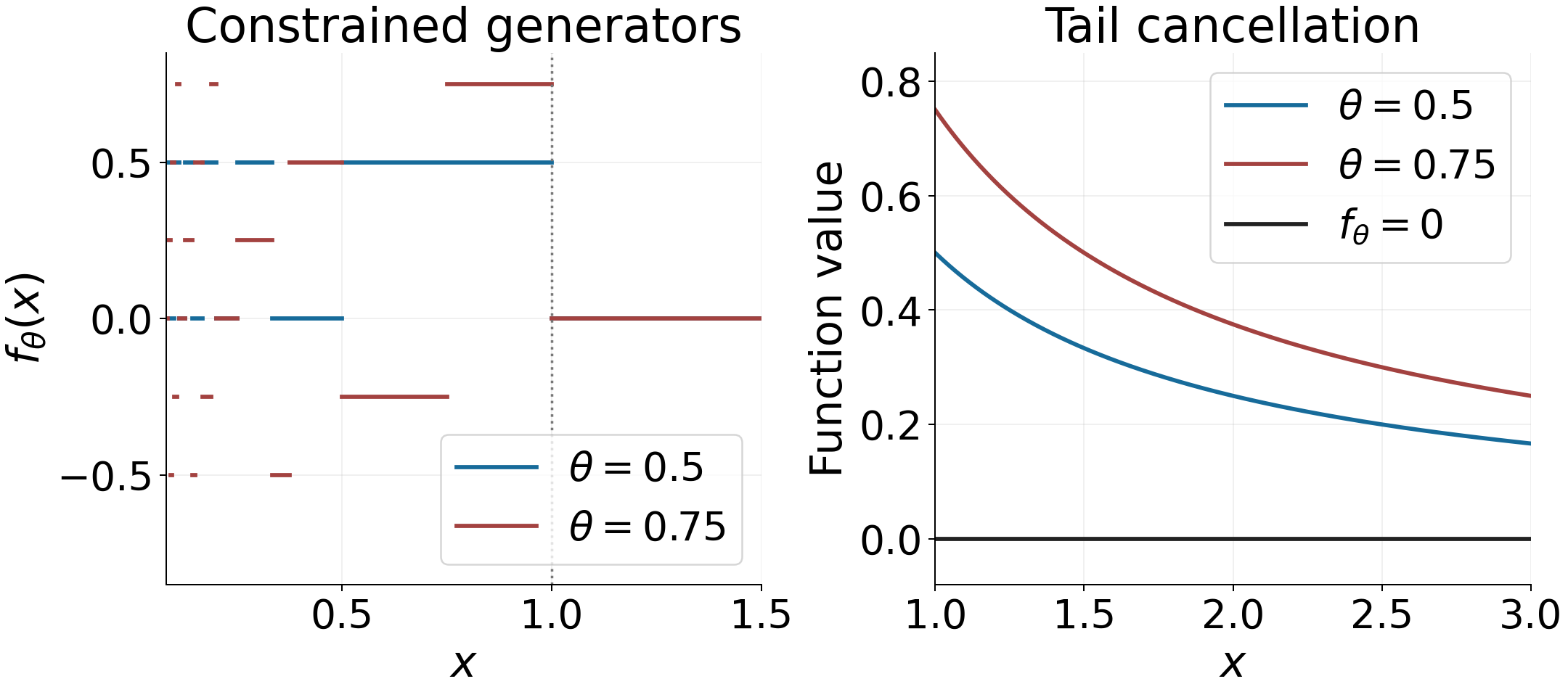
Figure 1. Left: exact generators (7.1), $\theta=1/2,3/4$, on $0.08<x<1.5$; jump endpoints are immaterial in $L^2$. Right: tails $\theta/x$ and their constrained cancellation for $x>1$. Individual graphs do not establish density.
Theorem 7.1 (Nyman–Beurling). RH holds if and only if the span of the functions (7.1) is dense in $L^2(0,1)$. Equivalently, the constant function one belongs to its closure.
We give the analytic ingredients before the proof. The method follows the Möbius approximation of Báez-Duarte and its analytic treatments by Burnol and Bagchi. A smoothed finite sum supplies the uniform estimate needed here.
Lemma 7.2 (Mellin isometry and the fractional parts). On the line $s=1/2+it$, the Mellin transform $$ \mathcal Tf(s)=\int_0^\infty f(x)x^{s-1}\,dx $$ extends to an isometry from $L^2(0,\infty;dx)$ onto $L^2(\mathbb R,dt/(2\pi))$. If $f$ is supported in $(0,1)$, its transform is also a holomorphic function for $\Re s>1/2$, and evaluation there is continuous. Moreover $$ \mathcal Tf_\theta(s)=-\frac{\zeta(s)}s(\theta^s-\theta) \qquad(\Re s>1/2), \tag{7.2} $$ with the removable value at one.
Proof. Set $x=e^u$ and $h(u)=e^{u/2}f(e^u)$. Then $\int|h|^2du=\int|f|^2dx$, and the Mellin transform on the indicated line is the Fourier transform $\int h(u)e^{itu}du$.
Here is the norm identity needed for that transform. Initially take smooth compactly supported $h$. Multiplying the squared Fourier transform by $e^{-\eta t^2}$ and applying Fubini gives $$ \frac1{2\pi}\int|\widehat h(t)|^2e^{-\eta t^2}dt =\int h(u)\overline{(h*K_\eta)(u)}du, \quad K_\eta(v)=\frac{e^{-v^2/(4\eta)}}{\sqrt{4\pi\eta}}. $$ The Gaussian Fourier integral follows from the Gaussian calculation in the theta lesson. $K_\eta$ has integral one and concentrates at zero; splitting at $|v|=r$ proves $h*K_\eta\to h$ in $L^2$. Monotone convergence on the left gives the norm identity. Density extends the transform isometrically to $L^2$. Applying the inverse transform with the same Gaussian cutoff recovers every smooth compactly supported function, so the range, which is closed, is dense and hence all of $L^2$. This proves the isometry.
For support in $(0,1)$, Cauchy–Schwarz gives $$ |\mathcal Tf(s)|\le\frac{\|f\|_2}{\sqrt{2\sigma-1}}. \tag{7.3} $$ On compact subsets with $\sigma>1/2$, the same estimate with additional powers of $|\log x|$ permits differentiation and proves holomorphy. For $\sigma>1$, summing the intervals where $\lfloor\theta/x\rfloor$ is constant gives $$ \int_0^1\{\theta/x\}x^{s-1}dx =\frac\theta{s-1}-\frac{\theta^s\zeta(s)}s. $$ One can equivalently write $\lfloor\theta/x\rfloor=\sum_{k\ge1}\mathbf1_{x\le\theta/k}$ and integrate the absolutely convergent sum. Subtract the case $\theta=1$ multiplied by $\theta$. The pole terms cancel, giving (7.2); holomorphic continuation extends it to $\sigma>1/2$, and the bounded fractional parts give its boundary values. $\square$
Lemma 7.3 (a smoothed reciprocal approximation). Assume RH, fix $0<\epsilon<1/4$ and $0<\eta<1$, and put $$ P_{\epsilon,N}(s)=\sum_{n\le N}\frac{\mu(n)}{n^{s+\epsilon}}(1-n/N). $$ For $s=1/2+it$, $$ P_{\epsilon,N}(s)=\frac1{\zeta(s+\epsilon)} +O_{\epsilon,\eta}(N^{-\epsilon/2}\tau^\eta). \tag{7.4} $$
Proof. The absolutely convergent kernel integral, for $c>0$, is $$ \frac1{2\pi i}\int_{c-i\infty}^{c+i\infty} \frac{y^w}{w(w+1)}dw=(1-y^{-1})_+. $$ For $y>1$, close to the left and take residues at zero and minus one; for $0<y<1$, close to the right. The horizontal integrals vanish by the quadratic denominator, followed by the outer vertical line. At $y=1$, the integral is zero by continuity, justified by its integrable majorant on the fixed line. Choosing $c=2$ and using the absolutely convergent reciprocal series gives $$ P_{\epsilon,N}(s)=\frac1{2\pi i}\int_{2-i\infty}^{2+i\infty} \frac{N^w}{w(w+1)\zeta(s+\epsilon+w)}dw. $$ Shift to $\Re w=-\epsilon/2$. Under RH the reciprocal is holomorphic in the intervening half-plane, including its removable zero at one. Only the kernel pole at zero is crossed, with residue $1/\zeta(s+\epsilon)$. Theorem 3.2 bounds the integrand on the new line by $$ C_{\epsilon,\eta}N^{-\epsilon/2} \frac{(|t+v|+4)^\eta}{1+v^2}. $$ Since $|t+v|+4\le\tau(1+|v|)$ and $\eta<1$, its integral is $O(N^{-\epsilon/2}\tau^\eta)$. The same bound on horizontal segments is $O_{N,t}(V^{\eta-2})$ as their heights $V$ tend to infinity, justifying the shift. $\square$
Lemma 7.4 (a uniform zeta ratio). Under RH, on $s=1/2+it$, $$ \left|\frac{\zeta(s)}{\zeta(s+\epsilon)}\right| \le C\tau^{\epsilon/2}\qquad(0<\epsilon\le1/4). \tag{7.5} $$
Proof. Write $\xi(s)=\tfrac12s(s-1)\pi^{-s/2}\Gamma(s/2)\zeta(s)$. Its functional equation makes $w\mapsto\xi(1/2+w)$ even. Its Hadamard product, proved in the entire-function lesson, therefore takes the paired form $$ \xi(1/2+w)=\xi(1/2)\prod_{\gamma>0}(1+w^2/\gamma^2) $$ under RH, with multiplicities. The sum $\sum\gamma^{-2}$ converges; pairing the genus-one factors leaves an exponential of degree at most one, whose linear term vanishes by evenness. There is no zero at $1/2$, since zeta has no real zero in $(0,1)$ by the alternating-series identity. For $w=it$, each factor has modulus no larger than its value at $w=\epsilon+it$, because $$ |\gamma^2+(\epsilon+it)^2|^2-(\gamma^2-t^2)^2 =2\epsilon^2(\gamma^2+t^2)+\epsilon^4\ge0. $$ Taking the limits of the paired products gives $|\xi(s)/\xi(s+\epsilon)|\le1$. Restoring the other factors gives $$ \left|\frac{\zeta(s)}{\zeta(s+\epsilon)}\right| \le\pi^{-\epsilon/2} \left|\frac{(s+\epsilon)(s+\epsilon-1)}{s(s-1)}\right| \left|\frac{\Gamma((s+\epsilon)/2)}{\Gamma(s/2)}\right|. $$ The rational factor is bounded uniformly on this line and range of $\epsilon$. The uniform Stirling formula bounds the gamma ratio by $C\tau^{\epsilon/2}$ at large heights; compactness covers the remaining heights since the gamma arguments stay away from poles. This proves (7.5). $\square$
Proof of Theorem 7.1. Assume RH. For fixed $\epsilon$, take the finite constrained sums $$ g_{\epsilon,N}(x)=-\sum_{n\le N}\mu(n)n^{-\epsilon}(1-n/N)f_{1/n}(x). $$ By (7.2), their Mellin transforms on the critical line are $$ \frac{\zeta(s)}s\bigl(P_{\epsilon,N}(s)-P_{\epsilon,N}(1)\bigr). $$ As $N\to\infty$, $P_{\epsilon,N}(1)\to1/\zeta(1+\epsilon)$ by absolute convergence. Lemma 7.3, with $\eta=1/16$, shows that the transforms converge in $L^2$ to $$ G_\epsilon(s)=\frac{\zeta(s)}s \left(\frac1{\zeta(s+\epsilon)}-\frac1{\zeta(1+\epsilon)}\right). \tag{7.6} $$ Indeed the error in (7.4), multiplied by $\zeta(s)/s$, has a square-integrable majorant: the proved convexity bound gives $\zeta(1/2+it)\ll\tau^{1/4+1/16}$, so the product is $O(\tau^{-5/8})$. The constant-term error multiplies the square-integrable function $\zeta(s)/s$. The isometry therefore makes (7.6) the transform of a member of the closed constrained span.
Now let $\epsilon\downarrow0$. Except at the discrete zeros on the line, $\zeta(s)/\zeta(s+\epsilon)\to1$, and the simple pole at one gives $1/\zeta(1+\epsilon)\to0$. Thus (7.6) tends to $1/s$ almost everywhere. Lemma 7.4 bounds its first term uniformly by $C\tau^{-7/8}$. Its second term is bounded by $C|\zeta(s)/s|$, also square-integrable. Dominated convergence gives $G_\epsilon\to1/s$ in $L^2$. Since $1/s$ is the transform of $\mathbf1_{(0,1)}$, the constant one belongs to the closed span.
Conversely, suppose one belongs to that closure and let $\rho$ be a zero with $\Re\rho>1/2$. Equation (7.2) says that every constrained finite sum has Mellin transform zero at $\rho$. The evaluation bound (7.3) preserves that zero under $L^2$ limits. But the transform of one at $\rho$ is $1/\rho\ne0$. This contradiction excludes such a zero; symmetry gives RH.
Finally, membership of one in the closure implies density. Extend all functions by zero beyond one. For $0<a\le1$, the bounded dilation $D_a f(x)=f(x/a)$ has norm $\sqrt a\|f\|_2$ and preserves the span, since $$ D_af_\theta=f_{a\theta}-\theta f_a. $$ Hence its closure contains $D_a\mathbf1_{(0,1)}=\mathbf1_{(0,a)}$ for every $a$. Differences give all interval step functions, which are dense in $L^2(0,1)$ by approximation of square-integrable functions by simple functions and intervals. Density trivially implies membership of one, proving all the assertions. $\square$
8. Positivity and the Lindelöf hypothesis
Li's criterion encodes the zero locations in a sequence of real numbers, $$ \lambda_n=\sum_\rho\left[1-(1-1/\rho)^n\right] =\frac1{(n-1)!}\left.\frac{d^n}{ds^n}[s^{n-1}\log\xi(s)]\right|_{s=1}. \tag{8.1} $$ The zero sum is symmetric in height and retains multiplicities. RH is equivalent to $\lambda_n\ge0$ for every $n\ge1$. The equality of the definitions and the criterion are proved in Li's criterion, Proposition 1.1 and Theorem 3.2. That lesson also proves the positive-coefficient singularity theorem needed for the converse. A finite list of positive coefficients cannot replace the universal condition.
Weil's criterion instead uses a quadratic form on test functions. With Mellin transform $\widetilde g(s)=\int_0^\infty g(x)x^{s-1}dx$, its zero form is $$ Q(g)=\sum_\rho\widetilde g(\rho) \overline{\widetilde g(1-\bar\rho)}. \tag{8.2} $$ Under RH, this becomes $\sum_\rho|\widetilde g(\rho)|^2\ge0$. An exact test class is the space $\mathcal G$ for which $h(u)=g(e^u)$ is smooth and $e^{a|u|}h^{(k)}(u)$ is bounded for every $a>0$ and $k\ge0$. RH is equivalent to $Q(g)\ge0$ for every $g\in\mathcal G$; the proof, including the converse built from Gaussians, is Weil's proof for curves and what is missing over the integers, Theorem 6.4. The compact-support criterion is proved in Weil's positivity criterion, Lemma 3.1 and Theorem 4.1. Its compact interpolation construction includes exact vanishing at any admissible finite set; take that set to be $\{0,1\}$. Thus $g\in C_c^\infty(\mathbb R_+^*)$, with $\widetilde g(0)=\widetilde g(1)=0$, and RH is equivalent to $Q(g)\ge0$ for every such $g$. The explicit formula expresses this form through local terms with only finitely many primes for each test function. The sign of a local distribution depends on the normalization; the zero form (8.2) fixes the sign used here.
The Lindelöf hypothesis is the assertion $\zeta(1/2+it)\ll_\varepsilon\tau^\varepsilon$ for every $\varepsilon>0$. It concerns growth on the line, whereas RH concerns all zero locations. The relation between these assertions is studied further in Growth on the critical line, Section 2; that later lesson supplies its own argument. The reciprocal estimate in Theorem 3.2 already supplies one analytic ingredient for that later proof.
9. Numerical evidence and the finite-field theorem
A finite verification needs a lower count on the critical line and an upper count for all zeros in the same region. Set $F(t)=\xi(1/2+it)$; conjugation and the functional equation proved in Poisson summation, theta and the functional equation make $F$ continuous and real. Fix a positive height with no boundary zero. If $F$ has certified opposite signs at the endpoints of each of $m$ disjoint intervals, continuity gives at least $m$ distinct critical-line zeros. If a certified argument-principle calculation gives at most $m$ nontrivial zeros in that region, counted with multiplicity, the counts agree. An omitted zero, an off-line pair or an extra multiplicity would increase the total, so every zero there is simple and on the line. The argument principle is proved in Dirichlet series and Euler products, Appendix A. Sample signs alone supply only the lower count. Every fixed finite height leaves larger heights outside its conclusion.
The geometric analogue is a theorem. For a smooth projective geometrically connected curve $C/\mathbb F_q$ of genus $g$, $$ Z(C,T)=\frac{\prod_{j=1}^{2g}(1-\alpha_jT)}{(1-T)(1-qT)}, \qquad |\alpha_j|=\sqrt q \tag{9.1} $$ under every complex embedding. Appendix B below proves the surface intersection, degree, duality and Hodge inputs. The remaining correspondence argument is proved in the earlier programme lesson Weil's proof for curves and what is missing over the integers, Sections 2–3, culminating in Theorem 3.12. Appendix B.5 gives the exact proof locators and matches their hypotheses. With $T=q^{-s}$, a numerator zero has $|T|=q^{-1/2}$, hence $\Re s=1/2$.
For higher dimensions, let $X_0/\mathbb F_q$ be smooth and projective, $X=X_0\times_{\mathbb F_q}\overline{\mathbb F}_q$, and $\ell\ne\operatorname{char}\mathbb F_q$. Deligne's theorem asserts that $$ \det(U-F\mid H^i_{\mathrm{\acute et}}(X,\mathbb Q_\ell))\in\mathbb Z[U] \tag{9.2} $$ is independent of $\ell$, and every complex conjugate $\alpha$ of an eigenvalue satisfies $|\alpha|=q^{i/2}$. Here $F$ has the geometric Frobenius convention, acting as $q^r$ on $\mathbb Q_\ell(-r)$. The full proof provider is The Riemann hypothesis over finite fields, Theorem 1.1 and Sections 5–6; it is already written. Its Section 6 proves integrality and independence of $\ell$, as well as purity. The historical statement is Deligne, La conjecture de Weil I, freely readable full text, Theorem (1.6). The apparently weaker all-conjugates purity statement is his Lemma (1.7); the integer-polynomial assertion is part of (1.6).
Thus the analogy supplies a proved geometric model. It does not transfer that theorem to the ordinary Riemann zeta function: the finite-field proof uses geometric structures whose arithmetic counterparts require their own construction.
10. Exercises with solutions
Exercise 1 (easy). Suppose $\psi(x)-x\ll_\varepsilon x^{1/2+\varepsilon}$ for every $\varepsilon>0$. Prove the same bound for $\theta(x)-x$.
Solution. The prime-power comparison gives $0\le\psi(x)-\theta(x)\ll\sqrt x$. Subtract it from $\psi(x)-x$ and apply the triangle inequality. Since $\sqrt x\le x^{1/2+\varepsilon}$ for $x\ge1$, the requested bound follows for each $\varepsilon$.
Exercise 2 (medium). Prove that RH is equivalent to $M(x)=O_\varepsilon(x^{1/2+\varepsilon})$ for every $\varepsilon>0$. Identify why nonvanishing alone is insufficient for the forward direction.
Solution. Under RH, Theorem 3.2 supplies the reciprocal growth bound. Apply bounded-coefficient Perron at the half-integer $X=\lfloor x\rfloor+1/2$ with $T=X$ and shift to $\sigma=1/2+\varepsilon/4$. With reciprocal exponent $\varepsilon/4$, the vertical integral is $O_\varepsilon(X^{1/2+\varepsilon/2})$, the horizontal integrals are $O_\varepsilon(X^{\varepsilon/4}/\log X)$, and the Perron error is $O(\log X)$. There is no residue. This is the desired bound, exactly as justified in Theorem 4.1. Nonvanishing permits the shift but does not bound its integrals.
Conversely, the asserted estimates make $s\int_1^\infty M(u)u^{-s-1}du$ holomorphic in $\sigma>1/2$: on a compact set choose an exponent smaller than its distance from the boundary. It equals $1/\zeta(s)$ for $\sigma>1$, hence its product with zeta is identically one by continuation. A zero in $\sigma>1/2$ would contradict this identity. Reflection symmetry then gives RH.
Exercise 3 (medium). Derive the von Koch bound for $\pi$ from the RH bound for $\psi$.
Solution. Remove the $O(\sqrt x)$ prime-power contribution to get $\theta(x)=x+O(\sqrt x\log^2x)$. Insert this in the exact partial-summation identity $\pi(x)=\theta(x)/\log x+\int_2^x\theta(u)/(u\log^2u)du$. The endpoint error is $O(\sqrt x\log x)$ and the integral error is $O(\sqrt x)$. The main term is $\operatorname{Li}(x)+2/\log2$, whose constant difference from $\operatorname{li}(x)$ is absorbed. Therefore $\pi(x)=\operatorname{li}(x)+O(\sqrt x\log x)$.
Exercise 4 (medium). If $\sum\mu(n)n^{-s}$ converges at a complex point $s_0$ with $\sigma_0<1$, show that zeta has no zero in $\sigma>\sigma_0$.
Solution. The partial sums $B(N)=\sum_{n\le N}\mu(n)n^{-s_0}$ are bounded. Partial summation of $\sum\mu(n)n^{-s_0}n^{-(s-s_0)}$ gives tails bounded on a compact set $K\subset\{\sigma>\sigma_0\}$ by $C_KN^{-d}$, where $d=\min_K\Re(s-s_0)>0$. Thus the sum defines a holomorphic function there. It agrees with $1/\zeta$ in $\sigma>1$, and meromorphic continuation makes its product with zeta identically one. At a zero this would give $0=1$. The conclusion concerns the open half-plane, with no claim on its boundary.
Exercise 5 (hard). Prove Grönwall's maximal-order theorem using Mertens' third theorem. Check that the lower-bound construction has the correct iterated-logarithm scale.
Solution. For the upper bound put $y=\log n$. The Euler product gives $\sigma_1(n)/n<\prod_{p\mid n}(1-1/p)^{-1}$. Primes at most $y$ contribute at most $(e^\gamma+o(1))\log y$. The $k$ larger prime factors obey $k\log y\le y$, so their product has logarithm at most $2k/y\le2/\log y=o(1)$. This proves the upper limsup $e^\gamma$.
For the lower bound take $a_y=\lceil\log y\rceil$ and $n_y=\prod_{p\le y}p^{a_y}$. The factors $1-p^{-a_y-1}$ have product tending to one because their missing-factor sum is $O(2^{-a_y})$. Mertens then gives $\sigma_1(n_y)/n_y\sim e^\gamma\log y$. Chebyshev's estimates give $\log n_y=a_y\theta(y)\asymp a_yy$, whence $\log\log n_y=\log y+\log a_y+O(1)\sim\log y$. Dividing proves the matching lower limsup. All uniform and endpoint details are in Theorem 5.1.
Appendix B. Surface and curve inputs for the geometric theorem
This appendix supplies the intersection, degree and Hodge arguments used by the curve theorem in Section 9. The cohomology and local algebra inputs are proved in the earlier programme lessons listed below. Each row names the precise written proofs and the hypotheses used here.
| Name used below | Earlier programme lesson and proof locator | Use |
|---|---|---|
| Serre | Serre's theorems on projective schemes, Theorems 2.1–2.2 | Eventual vanishing of higher cohomology and global generation for ample twists on proper schemes. |
| Coherent | Coherence of higher direct images under proper morphisms, Lemma 1.2, Theorems 2.2 and 4.1, Corollary 5.1 | Extension across a closed complement, coherent filtrations and finite-dimensional proper cohomology on Noetherian schemes. |
| Euler | Euler characteristics and Hilbert polynomials, Proposition 1.1, field-extension calculation after Proposition 1.2, Theorems 2.1 and 3.1 | Additivity, field extension, polynomial Euler characteristics and positivity for ample twists. |
| Affine | Affine cohomology and Serre's criterion, Theorems 2.2, 3.1, 3.2, 4.3 and 5.2, Corollary 5.3 | Affine vanishing, finite-cover computation, direct images and the finite-ideal affine criterion. |
| Formal | The theorem on formal functions, Corollary 4.2 and the final two paragraphs of Theorem 5.2's proof | Completed proper direct images and the affine/coherent argument for finiteness. |
| Duality | Dualizing sheaves and Serre duality for projective schemes, Lemma 2.1, equations (6)–(8), Theorems 4.1–4.2 and the local calculation in Theorem 5.1 | Projective equidimensional Cohen–Macaulay duality and the local Koszul identification. |
| Ambient canonical line | Ext sheaves and Serre duality on projective space, solution to Exercise 7.4 | The Euler-sequence determinant calculation of the canonical line on projective space. |
| Regular | Regular local rings, Theorem 1.1, Proposition 1.4 and solution to Exercise 7.2 | Regular local rings are Cohen–Macaulay domains; regular quotients and the one-dimensional DVR calculation. |
| Koszul | Projective dimension and the Auslander–Buchsbaum formula, Theorem 4.1 | The Koszul resolution of a regular sequence. |
| Dimension | Krull dimension and Noether normalization, Theorems 4.2, 4.3 and 6.1 | Finite-type dimensions, finite residue fields at closed points, and zero-dimensional proper closed subsets of integral curves. |
| Differentials | Kähler differentials, Theorems 2.1, 3.3 and 4.1, Proposition 5.2 | Base change, the conormal sequence and the diagonal conormal identification. |
| Smooth | Formally smooth, unramified and étale ring maps, Theorems 1.2, 3.1, 4.1 and 5.1 | Base change, composition and the locally split smooth conormal sequence. |
| Smooth | Smooth algebras over a field and the Jacobian criterion, Theorem 2.1 | Regularity and locally free differentials of the expected rank. |
B.1. Mixed Euler differences and intersection numbers
Let $X$ be proper over a field $k$. For a coherent sheaf $F$ and an invertible sheaf $N$, put $$ a_F(N)=\chi(X,F\otimes N),\qquad \Delta_L a_F(N)=a_F(N\otimes L)-a_F(N). $$ The Euler characteristic is finite by Coherent and a finite affine-cover complex. The difference operators commute, because tensor products of invertible sheaves commute.
Lemma B.1. If the support of $F$ has dimension at most $d$, then every product of $d+1$ operators $\Delta _L$ annihilates $a_F$, at every invertible base twist $N$.
Proof. For zero-dimensional support, the closed scheme cut out by the annihilator is finite over $k$. Indeed it has finitely many points, each open, with local Artinian coordinate ring and finite residue extension; its nilpotent filtration makes each coordinate ring finite-dimensional. An invertible module over a local Artinian ring is free of rank one. Twisting therefore preserves the dimension of global sections and higher cohomology is zero. Thus every first difference vanishes.
Proceed by induction on support dimension. By Coherent, Theorem 2.2, and Euler additivity it suffices to treat a nonzero coherent ideal $I$ on an integral closed subscheme $V$. For a fixed $L$, choose a generic isomorphism from $I$ to $I\otimes L$. Coherent, Lemma 1.2, extends it to a map from $E=J^a I$, where $J$ cuts out a closed complement of a dense open. This map and the inclusion into $I$ are injective: their kernels are generically zero subsheaves of a torsion-free module on the integral scheme. Both cokernels $Q,Q'$ have support dimension less than $\dim V$. Tensoring their exact sequences with any $N$ gives $$ \Delta_L a_I(N)=a_{Q'}(N)-a_Q(N). $$ By induction, any further $d$ mixed differences annihilate the right-hand side. Reassembling the filtration proves the assertion. This argument proves mixed differences directly; the twists need not be ample. $\square$
Consequently, for line bundles $L_1,...,L_r$, the function $$ (n_1,\ldots,n_r)\longmapsto \chi(X,F\otimes L_1^{n_1}\otimes\cdots\otimes L_r^{n_r}) $$ is a numerical polynomial of total degree at most $d$ on all of $\mathbb Z^r$. To justify this last step, apply the commuting forward differences in the standard coordinate directions. Successive discrete integration in the basis $\binom{n_i}{j}$ gives $$ \sum_{|\alpha|\le d}(\Delta_1^{\alpha_1}\cdots \Delta_r^{\alpha_r}a)(0)\prod_i\binom{n_i}{\alpha_i}. $$ The difference equations determine equality first on nonnegative integers and then backwards on negative integers. All differences of total order greater than $d$ vanish by Lemma B.1. This proves both the polynomial formula and its total-degree bound.
On a proper surface $S$, define $$ (L\cdot M)=\chi(L\otimes M)-\chi(L)-\chi(M)+\chi(\mathcal O_S). \tag{B.1} $$ This is an integer. Every third mixed difference vanishes, so $\Delta _L \Delta _M \chi (N)$ is independent of the invertible base twist $N$. It is symmetric. The operator identity $$ \Delta_{L_1\otimes L_2}=\Delta_{L_1}+T_{L_1}\Delta_{L_2}, \qquad (T_La)(N)=a(N\otimes L), $$ together with that independence proves additivity in $L$; symmetry proves additivity in $M$. Negative powers are included. Thus (B.1) is a symmetric bilinear form on $\operatorname{Pic}(S)$, and extends to $\operatorname{Pic}(S)\otimes\mathbb Q$.
In particular, the coefficient of $mn$ in $\chi (L^m\otimes M^n)$ is $(L\cdot M)$. The one-variable formula is $$ \chi(L^n)=\chi(\mathcal O_S) +n\bigl(\chi(L)-\chi(\mathcal O_S)\bigr) +\binom n2(L\cdot L) =\tfrac12(L\cdot L)n^2+O(n). \tag{B.2} $$ This supplies (S1), including symmetry, integrality and bilinearity; no surface Riemann–Roch formula has been assumed.
B.2. Curve degrees and restriction to a Cartier divisor
For a proper scheme $D$ of dimension at most one and an invertible sheaf $A$, define $$ \deg_D A=\chi(D,A)-\chi(D,\mathcal O_D). $$ Lemma B.1 with $d=1$ gives $$ \deg_D(A\otimes B)=\deg_D A+\deg_D B. \tag{B.3} $$ This holds also for a nonreduced or reducible $D$, and proves (C1).
If $Z$ is an effective Cartier divisor on a proper integral curve $D$, it is zero-dimensional and finite. The exact sequence $$ 0\longrightarrow\mathcal O_D\longrightarrow\mathcal O_D(Z) \longrightarrow\mathcal O_D(Z)|_Z\longrightarrow0 $$ and the local Artinian calculation in B.1 imply $$ \deg_D\mathcal O_D(Z)=\dim_k\Gamma(Z,\mathcal O_Z)>0 \quad(Z\ne\varnothing). \tag{B.4} $$ The same reasoning shows $h^0(Z,A|_Z)=\dim_k \Gamma (Z,\mathcal O_Z)$ for any invertible $A$. If $D$ is smooth and $P$ is a closed point, Regular's DVR calculation makes $P$ a Cartier divisor, and (B.4) gives $\deg \mathcal O_D(P)=[k(P):k]$. This proves (C2). A nonzero section on an integral curve gives an effective Cartier zero divisor (possibly empty); hence a line bundle of negative degree has no nonzero section.
Every invertible sheaf on a smooth integral proper curve has the form $\mathcal O_D(E)$ for a divisor $E$. Indeed, choose a nonzero rational section. In a local trivialization its valuation at each closed point is defined by the DVR calculation in Regular. Only finitely many valuations are nonzero, because the section and its inverse are regular on a common dense open and its complement is a finite set. Multiplication by the rational section identifies the local lattice of $\mathcal O_D(E)$ with the given line bundle. This also proves that its Euler degree equals the sum of the valuations weighted by residue degrees.
Lemma B.2 (degree under a finite curve map). For a nonconstant proper $k$-morphism $f:D'\to D$ of integral curves, put $e=[k(D'):k(D)]$. Then $f$ is finite and $$ \deg_{D'}f^*A=e\deg_D A. \tag{B.5} $$ No separability hypothesis is imposed.
Proof. The function-field extension is finite by Dimension. Each closed fibre is a proper closed subset of the integral source curve, hence has dimension zero and finitely many points; the generic fibre has dimension zero as well. To use Formal without an external vanishing assertion, consider any infinitesimal fibre $X_n$ over a Noetherian local Artinian quotient of a base local ring. Its underlying space is a finite zero-dimensional fibre. Each point is open and admits a singleton affine neighbourhood; therefore $X_n$ is a finite disjoint union of affine schemes and is affine. Affine vanishing gives $H^q(X_n,G_n)=0$ for every coherent $G_n$ and $q>0$. Formal, Corollary 4.2, makes the completed stalk of $R^qf_*G$ zero. Coherent finiteness and Nakayama make the uncompleted stalk zero. Over an affine open in $D$, Leray and the finite-ideal version of Affine's Serre criterion then make the inverse image affine. Its coordinate ring is finite over the base ring by Coherent. This proves finiteness, reproducing precisely the needed case of Formal's Theorem 5.2 with its vanishing input proved here.
Now $E=f_*\mathcal O_{D'}$ is a torsion-free coherent sheaf of generic rank $e$. Choose a generic identification with $\mathcal O_D^e$. Extending it as in Coherent, Lemma 1.2, produces a common lattice embedded into both sheaves, with zero-dimensional cokernels. Tensoring these exact sequences by $A$ leaves the Euler characteristics of their cokernels unchanged. Subtracting before and after tensoring therefore gives $$ \chi(D,E\otimes A)-\chi(D,E) =e\bigl(\chi(D,A)-\chi(D,\mathcal O_D)\bigr). $$ For a finite map, higher direct images vanish by Affine, Theorem 3.2. Projection formula here is elementary: on an open where $A$ is free of rank one, $f_*f^*A=E\otimes A$, and these identifications agree under changes of frame. Proper pushforward of Euler characteristics now identifies the left side with $\deg_{D'} f^*A$. This proves (B.5), hence (C3). $\square$
If $D$ is an effective Cartier divisor on a proper surface $S$, the exact multiplication sequences give $$ \chi(N)-\chi(N(-D))=\chi(D,N|_D),\qquad \chi(\mathcal O_S)-\chi(\mathcal O_S(-D))=\chi(D,\mathcal O_D). $$ Compute $\Delta _N \Delta _{\mathcal O(D)} \chi$ at the base twist $\mathcal O(-D)$ and use its independence of the base twist from B.1. Subtraction gives $$ (N\cdot\mathcal O_S(D))=\deg_D(N|_D). \tag{B.6} $$ This proves (S2), also when $D$ is nonreduced or reducible.
B.3. Smooth duality, the conormal line and the genus
Let $X$ be smooth, projective and geometrically integral of dimension $n$ over $k$. Smooth and Regular show that it is equidimensional and Cohen–Macaulay, so Duality, Theorem 4.2, applies. We also need to identify its dualizing sheaf.
Embed $X$ in $P^N$. At a point of $X$, the ambient and quotient local rings are regular. Regular, Proposition 1.4, makes the embedding ideal locally a regular sequence of length $c=N-n$. Koszul's resolution and the local calculation in Duality give $$ \omega_X^\circ\cong \bigl(\det(I/I^2)\bigr)^\vee\otimes\omega_{P^N}|_X. $$ This calculation is local and does not require $X$ to be a global complete intersection. To see that it glues, replace a local regular generating list by another. Its matrix modulo $I$ changes the top Koszul generator by its determinant; the dual top Ext generator changes by the inverse determinant. These are exactly the transition functions of $(\det(I/I^2))^\vee$.
Differentials and Smooth give the locally split exact conormal sequence $$ 0\longrightarrow I/I^2\longrightarrow\Omega_{P^N/k}|_X \longrightarrow\Omega_{X/k}\longrightarrow0. $$ Taking determinants, and using the written ambient canonical-line calculation, identifies the last displayed dualizing line with $\det \Omega _{X/k}$. Thus for an invertible $A$, Duality gives $$ H^i(X,A)^\vee\cong H^{n-i}(X,A^{-1}\otimes\det\Omega_{X/k}). \tag{B.7} $$ It also supplies vanishing above dimension $n$ in this smooth projective case.
For a smooth projective geometrically integral curve $C$, $H^0(C,\mathcal O_C)=k$. Indeed, it is a finite-dimensional domain by Coherent, hence a finite field extension of $k$. Field extension in Euler identifies its tensor product with an algebraic closure with the global functions of the integral curve over that closure. A finite-dimensional domain over an algebraically closed field is that field, so its original dimension is one. Put $g=h^1(C,\mathcal O_C)$. Taking $A=\mathcal O_C$ and $A=\Omega _{C/k}$ in (B.7) gives $h^0(\Omega )=g$ and $h^1(\Omega )=1$. Consequently $$ \deg_C\Omega_{C/k}=(g-1)-(1-g)=2g-2, $$ and the definition of degree and (B.7) give the curve Riemann–Roch formula $$ h^0(C,A)-h^0(C,\Omega_{C/k}\otimes A^{-1}) =\deg_C A+1-g. \tag{B.8} $$ This supplies the Riemann–Roch input of the written curve-zeta rationality proof as well.
For every effective Cartier divisor $D$ on $S$, its ideal is $\mathcal O_S(-D)$, so its conormal sheaf is $$ I_D/I_D^2=\mathcal O_S(-D)|_D. $$ For the diagonal in $C\times C$, Differentials, Theorem 4.1, gives $I_\Delta /I_\Delta ^2=\Omega _{C/k}$. The diagonal is a Cartier divisor: locally the ambient and quotient are regular, of codimension one, so Regular, Proposition 1.4, makes its ideal principal with a nonzerodivisor generator. Combining these assertions with (B.6) gives $$ (\Delta\cdot\Delta)=-\deg_C\Omega_{C/k}=2-2g. $$ These assertions prove (C4), with the sign required in the correspondence proof.
B.4. The Hodge consequence, including its equality case
Let $S$ be a smooth projective geometrically integral surface. We first prove the assertion for a very ample integral hyperplane section, then extend it to any class of positive square.
An integral hyperplane section can be obtained after a purely transcendental field extension without invoking a Bertini theorem. Embed $S$ by a very ample line bundle in $P^N$. The incidence variety $$ I=\{(x,h)\in S\times(P^N)^\vee:x\in h\} $$ is a projective bundle over $S$: at $x$, hyperplanes through $x$ form the projectivization of the kernel of the evaluation map from the constant space of linear forms onto the very ample line at $x$. Thus $I$ is integral. Its projection onto the dual projective space is dominant. Every hyperplane meets $S$, since otherwise $S$ would be a proper affine positive-dimensional scheme, whereas proper coherence makes the coordinate ring of such a scheme finite-dimensional and hence zero-dimensional. The generic fibre of this dominant morphism between integral schemes is integral: on affine charts its coordinate rings are localizations of domains. Its dimension is one, either by the function-field dimension formula or by $\dim I=N+1$ and $\dim((P^N)^\vee)=N$. Over $K=k((P^N)^\vee )$, write this generic hyperplane section as $H$. It is an effective Cartier divisor because a nonzero hyperplane equation is a nonzerodivisor on the integral surface.
Field extension in Euler preserves every Euler characteristic, and consequently all intersection numbers from (B.1). Smoothness and geometric integrality also persist. It suffices to establish the desired numerical inequalities after this extension. In the rest of the proof we work over $K$, and omit it from the notation.
By (B.6), $$ H^2=\deg_H\mathcal O_S(H)|_H>0. $$ The positivity follows from Euler, Theorem 3.1: the Euler polynomial of an ample line on a nonzero proper one-dimensional scheme has a positive linear coefficient, and that coefficient is its degree by (B.3). More generally, for any nonzero effective Cartier divisor $B$ on $S$, $$ H\cdot B=\deg_B\mathcal O_S(H)|_B>0. \tag{B.9} $$ Here $B$ may be nonreduced or reducible; its dimension is one, and Euler's positivity theorem applies to $\mathcal O_B$.
We need a section bound on the integral curve $H$ that depends only on degree. Choose a nonempty effective Cartier divisor $Z$ on $H$. Such a choice requires no smoothness of $H$: choose a closed point $x$, an ample line $A$ and a sufficiently large power. Euler positivity and Serre, Theorem 2.2, make $h^0(A^m)$ grow, while evaluation at $x$ has target of dimension $[k(x):K]$. A nonzero section in its kernel has a nonempty finite Cartier zero divisor $Z$, because $H$ is integral. Put $a=\dim_K \Gamma (Z,\mathcal O_Z)>0$. For a line bundle $B$ on $H$ of degree $d\ge 0$, take $j=\lfloor d/a\rfloor+1$. Repeatedly apply $$ 0\longrightarrow B(-(i+1)Z)\longrightarrow B(-iZ) \longrightarrow B(-iZ)|_Z\longrightarrow0. $$ The last restriction has $a$ global sections, and $\deg B(-jZ)<0$ makes its global sections zero. Hence $$ h^0(H,B)\le a\bigl(\lfloor d/a\rfloor+1\bigr). \tag{B.10} $$ For $d<0$ it is zero. This proves a uniform bound for every fixed degree. It does not assume a rational point or a nonsingular hyperplane section.
Let $E$ be an integral line-bundle class with $E\cdot H=0$. If $\mathcal O_S(nE)$ has a nonzero section, its Cartier zero divisor is either empty or has positive intersection with $H$ by (B.9). Since $nE\cdot H=0$, that divisor must be empty. The section then trivializes the line bundle. Thus $$ h^0(S,\mathcal O_S(nE))\le h^0(S,\mathcal O_S) \quad(n\in\mathbf Z). \tag{B.11} $$ Let $\omega _S=\det \Omega _{S/K}$. By (B.7), $$ h^2(S,\mathcal O_S(nE))=h^0(S,\omega_S(-nE)). $$ Choose a fixed integer $j_0\ge 1$ with $\omega _S\cdot H-j_0 H^2<0$. A line bundle with negative intersection with $H$ has no nonzero section by (B.9), so $\omega _S(-nE-j_0H)$ has none. Restriction to $H$ repeatedly gives $$ h^0(S,\omega_S(-nE)) \le\sum_{j=0}^{j_0-1}h^0\bigl(H,\omega_S(-nE-jH)|_H\bigr). $$ The degree of its $j$th summand is $\omega _S\cdot H-jH^2$, independent of $n$. The bounds (B.10) therefore bound this sum independently of $n$. Since $h^1\ge 0$ and higher cohomology vanishes here, (B.11) implies an upper bound for $\chi (\mathcal O_S(nE))$ independent of $n$. Comparing with (B.2) forces $$ E\cdot H=0\quad\Longrightarrow\quad E^2\le0. \tag{B.12} $$ Clearing denominators extends this to rational classes.
If also $E^2=0$, let $F$ be any rational line-bundle class and put $$ F_0=F-\frac{F\cdot H}{H^2}H. $$ For every rational $t$, $(E+tF_0)\cdot H=0$, so (B.12) gives $$ 2t(E\cdot F_0)+t^2 F_0^2\le0. $$ Choosing sufficiently small rational $t$ of both signs forces $E\cdot F_0=0$; hence $E\cdot F=0$. This proves that a zero-square class in $H^\perp$ is numerically trivial.
Finally let $H'$ be any rational class with $H'^2>0$. There cannot be a two-dimensional rational subspace on which the intersection form is positive definite: that subspace would have a nonzero rational vector orthogonal to $H$, contradicting (B.12). If $L\cdot H'=0$ and $L^2>0$, the span of $H'$ and $L$ would be such a positive definite subspace. Therefore $L^2\le 0$. If $L^2=0$, apply this last nonpositivity to $$ L+t\left(F-\frac{F\cdot H'}{H'^2}H'\right) $$ for arbitrary $F$ and rational $t$. The same small-$t$ argument makes $L\cdot F=0$ for every class $F$. Conversely a numerically trivial class has square zero. We have proved the precise input (S3): $$ H'^2>0,\quad L\cdot H'=0 \quad\Longrightarrow\quad L^2\le0, \qquad L^2=0\iff L\text{ is numerically trivial}. \tag{B.13} $$ This argument establishes the numerical-triviality conclusion for original classes as well: all their pairings are unchanged by the field extension, so vanishing after extension implies their original pairings vanish.
B.5. Application to the existing complete curve-correspondence proof
A smooth geometrically connected curve is geometrically integral: its regular local rings are domains, so its irreducible components cannot meet; the finitely many components are therefore open and closed, and connectedness leaves just one. Smoothness also makes it reduced. For $C/\mathbb F_q$ smooth, projective and geometrically integral, $S=C\times C$ satisfies the hypotheses just used. We use the field-extension formulation of geometric integrality: the curve remains integral after every extension of its base field. For an affine product chart with coordinate domains $A,B$, the map $A\otimes B \to A\otimes \operatorname{Frac}(B)$ is injective because tensoring vector spaces over the base field is exact. Its target is a domain by geometric integrality of the first factor. Hence the product chart is integral. These charts have nonempty mutual overlaps, since nonempty opens in each integral curve meet, so the product is integral; the same argument after any field extension makes it geometrically integral. The product is smooth by Smooth's base-change and composition proofs. A product of projective embeddings is projective through the Segre map: on the chart with a nonzero product coordinate, the rank-one matrix relations recover the two sets of affine coordinates, so this map is a closed immersion. Thus the preceding statements apply without a genus or field-size restriction.
In Weil's proof for curves and what is missing over the integers, the inputs stated in Section 3.1 are now supplied as follows:
| Provider input | Proof in this appendix |
|---|---|
| (S1), multivariate Euler polynomial and integer symmetric bilinear intersection | B.1, Lemma B.1 and equations (B.1)–(B.2) |
| (S2), intersection by Cartier restriction | B.2, equation (B.6) |
| (S3), every positive-square class, including equality | B.4, equation (B.13) |
| (C1), additivity of curve degree | B.2, equation (B.3) |
| (C2), effective-divisor length and closed-point degree | B.2, equation (B.4) and the DVR paragraph |
| (C3), degree under any nonconstant proper integral-curve map | B.2, Lemma B.2; inseparability is allowed |
| (C4), Cartier conormal, diagonal conormal and degree $2g-2$ | B.3 |
| Curve Riemann–Roch and representation of line bundles by divisors | B.3, equation (B.8), and the rational-section paragraph of B.2 |
The remaining correspondence proof is already written, with these actual locators:
- Section 2, Theorems 2.3–2.4 and Corollary 2.5: finiteness of $\operatorname{Pic}^0$, existence of a degree-one class, rationality, functional equation and power-sum point counts. These use the curve Riemann–Roch formula supplied in (B.8), not an imported curve-RH theorem. Lemma 2.7 and Proposition 2.8 prove the power-sum criterion for the moduli of the reciprocal roots.
- Lemmas 3.1–3.4: Cartier pullback, graphs, fibre intersections and the two correspondence degrees. A finite-map graph is Cartier also directly: it is a smooth integral curve in the smooth surface, so Regular, Proposition 1.4, makes the codimension-one ideal generated by one nonzerodivisor. These lemmas use exactly (S1), (S2), (C1)–(C3).
- Lemmas 3.5–3.6: $\deg F^r=q^r$ by a function-field tower calculation, and the reduced fixed-point scheme by $a^{q^r}-a$. These are full written arguments and do not assume the Riemann hypothesis.
- Proposition 3.7: $(\Gamma _r\cdot \Gamma _s)=q^{\min(r,s)} N_{|r-s|}$, with $N_0=2-2g$, using the proved degree, restriction and conormal facts.
- Theorem 3.9: the trace pairing gives $\langle \Gamma _r,\Gamma _s\rangle =q^{\min(r,s)} \sum _j \alpha _j^{|r-s|}$.
- Theorem 3.10 and Corollary 3.11: set $V=p_1^*B_1$, $W=p_2^*B_1$. Their intersections are $V^2=W^2=0$, $V\cdot W=1$; hence $H'=V+W$ has square $2$. Equation (B.13) gives nonnegativity of the correspondence pairing and the exact equality criterion. Positivity for integer combinations extends to rational and real combinations, so its quadratic discriminant gives Cauchy–Schwarz.
- Theorem 3.12: $\langle \Delta ,\Gamma _r\rangle =q^r+1-N_r$, $\langle \Delta ,\Delta \rangle =2g$ and $\langle \Gamma _r,\Gamma _r\rangle =2g q^r$ give $$ |N_r-q^r-1|\le 2gq^{r/2}. $$ Proposition 2.8 then gives $|\alpha _j|=\sqrt q$, including the genus-zero case with no reciprocal roots.
These calculations supply the surface and degree inputs of the earlier written curve proof, and therefore establish the geometric statement (9.1).
Sources and attribution
The zero-boundary and prime-error comparison is Koukoulopoulos, The Distribution of Prime Numbers, freely readable author preliminary version, Chapter 6, Theorem 6.1. Bombieri, Problems of the Millennium: the Riemann Hypothesis, Sections II–IV, gives freely readable context. Sections 1–5 and 7 prove their results using the preceding lessons.
Sections 6.1–6.5 adapt Whidden, Robin's 1984 criterion for the Riemann hypothesis: a formally verified proof, release 1.1.1, revision acab1a31f31e0499518a4416b63281e0b4838f9c, under CC BY 4.0. The adaptation and changes are identified before Section 6.1. All arguments, 36 finite-cover rows and complete verification programs needed for Theorem 6.1 appear in this lesson. The exact integer programs and their original explanation are CC0. A second comparison is Lagarias, An elementary problem equivalent to the Riemann hypothesis, free author preprint, version 2, Theorem 1.1 and its proof. The course has executed its own finite certificates; it does not claim to have rerun the source's formal project.
Burnol, On an analytic estimate in the theory of the Riemann zeta function and a theorem of Báez-Duarte, free author preprint, Sections 2–3, and Bagchi, On Nyman, Beurling and Báez-Duarte's Hilbert space reformulation of the Riemann hypothesis, free author preprint, Lemma 3 and Theorems 2 and 5, explain analytic versions of the approximation criterion. The proof here supplies the complete smoothed estimate (7.4) and uses the earlier proved convexity bound.
Deligne, La conjecture de Weil I, freely readable full text, Theorem (1.6) and Lemma (1.7) is the free primary statement comparison for Section 9; its programme proof is located there. Connes, The Riemann Hypothesis: Past, Present and a Letter Through Time, free author preprint, version 1, surveys these formulations.
Exact source formula qualifications. In Lagarias, arXiv:math/0008177v2, the first display in the proof of Lemma 3.1 prints an infinite upper limit for the integral of $\lfloor t\rfloor/t^2$. For every integer $n\ge1$, the finite identity is $$ \int_1^n\frac{\lfloor t\rfloor}{t^2}\,dt =\sum_{r=1}^n\int_r^n\frac{dt}{t^2} =\sum_{r=1}^n\left(\frac1r-\frac1n\right)=H_n-1. $$ The first equality uses $\lfloor t\rfloor=\sum_{r=1}^n\mathbf1_{[r,\infty)}(t)$ on $[1,n)$; the endpoint has no effect on the integral. The infinite integral diverges, since $\lfloor t\rfloor\ge t/2$ for $t\ge2$. The source's next display, (3.4), has upper limit $n$ correctly. Section 6.5 supplies the lesson's own harmonic comparison and finite proof.
In Bagchi, arXiv:math/0607733v1, the proof of Theorem 2 drops the rational completion factor when asserting a uniform bound for $|\zeta(s)/\zeta(s+\epsilon)|$ on $\Re s\ge1/2$. For any fixed $0<\epsilon<1/2$ and $s=1+\delta$, $\delta\downarrow0$, the earlier proved Laurent expansion at one and continuity in $\Re s>1$ give $$ \frac{\zeta(1+\delta)}{\zeta(1+\epsilon+\delta)} \sim\frac1{\delta\zeta(1+\epsilon)}\longrightarrow+\infty. $$ Here $\zeta(1+\epsilon)>0$ by its convergent Dirichlet series, while $|1+\delta|^{\epsilon/2}$ stays bounded. Thus that larger-domain bound fails near the pole. Lemma 7.4 proves precisely the critical-line bound needed here, retaining the rational, gamma and $\pi$ factors. On that line its rational factor is uniformly bounded. This local source-domain correction does not contradict the approximation criterion.