Uniform complex stationary phase from exact critical-ideal division

This is the complete original analytic companion for U028. It keeps the historical attribution to Hörmander I, Theorems 7.7.1 and 7.7.12. The freely readable comparisons are Melin–Sjöstrand's 1974 seminar exposition and Sjöstrand's 1982 holomorphic stationary-phase proof. Neither free comparison, by itself, proves the complete smooth parameter contract below. The proof here uses the exact smooth complex division and positive critical-value results already proved in U028, Sections 2–5; it does not reopen U026.

The preserved nine-section proof has been checked for this restoration. The contour and Gaussian foundations add the finite matrix factorization, the exact deformation identity, the Gaussian branch and the residue-jet argument needed below. This revision is written in original words and notation. External primary PDFs are not redistributed here. Source-use and rights record distinguish the historical comparisons from the proof supplied here.

1. The exact contract

Let x range over a small real neighborhood of 0 in $\mathbb R^d$, and p range over a small real parameter neighborhood of 0. Let $f(x,p)$ be a smooth complex function such that

The zero imaginary value at the mark is automatic in the U028 application: the original homogeneous phase has a parameter critical point there, so Euler's identity makes its value zero, and subtracting a real Fourier linear phase leaves its imaginary part zero. If the imaginary value is strictly positive, a smaller patch has exponential decay and the stationary contribution is unnecessary.

The imaginary Hessian at the mark is only semipositive. It can have null directions. Nearby parameters need not have any real critical point; the real critical parameter set can be singular.

Write $I=(f_{x_1},\ldots,f_{x_d})$. The previously established complex division and critical-value argument provide, on one fixed patch,

A smooth amplitude $b(x,p,\lambda)$ is supported in one fixed compact real x patch and is bounded with every mixed derivative, including derivatives in an auxiliary parameter $\lambda$. $\lambda$ can range over a noncompact set. The large parameter $t\ge1$ is initially independent of $\lambda$. The U028 application substitutes $\lambda=\log t$ into its bounded normalized symbol family.

There are smooth residue operators $C_j$, linear in b and of amplitude differential order at most $2j$, with all parameter and $\lambda$ derivatives uniformly bounded, such that

and

These are absolute errors. The proof never divides an error by $e^{itf_0}$. For each requested L the estimates use finitely many seminorms of the amplitude, phase and chosen smooth residue/extension representatives, with fixed patch, Hessian-inverse and support bounds. The bounded-family construction gives these bounds on one patch. Arbitrary representatives may have different flat errors and different constants; no uniform estimate over uncontrolled choices of representatives is claimed. For phase families one must impose those quantitative bounds uniformly; the words "bounded family" alone do not supply a common invertibility radius.

The leading operator is the residue of

where the square root is the Gaussian branch. All cutoffs and neighborhoods are fixed by the phase geometry before the amplitude or L is chosen. This supports the all-order converse in U028.

Differentiating in p can differentiate the oscillatory factor and cost powers of t. A safe unfactored estimate is

Arbitrarily rapid auxiliary errors have arbitrarily rapid derivatives after increasing their construction order. Do not claim the same remainder exponent for an arbitrary p derivative without either increasing the truncation depth or specifying a covariant derivative removing the oscillatory phase. The U028 symbol argument needs bounded coefficient derivatives and the value estimate (P4), and has both.

2. A complete nonstationary proof

Let K be a fixed compact integration patch, f a bounded smooth phase family with $\operatorname{Im}f\ge0$, and

Choose a scalar smooth cutoff $\chi$, zero below $c/4$ and one above $c/2$. Split b into $\chi(\operatorname{Im}f)b$ and $(1-\chi(\operatorname{Im}f))b$. On the first support $\operatorname{Im}f\ge c/4$, so its integral is bounded by the compact-volume constant times $e^{-tc/4}$ times the amplitude supremum. Parameter derivatives produce only finitely many powers of t and remain rapid.

On the second support $|d_xf|^2\ge c/2$. There use

After k integrations by parts,

All denominators are bounded below uniformly. Derivatives of V and of the splitting cutoff use finitely many bounded phase derivatives, the lower bound c, and finitely many amplitude derivatives. Since $|e^{itf}|\le1$, the last integral is uniformly bounded. This proves $O(t^{-k})$ for every k. There are no boundary terms because the amplitudes are compactly supported. Choose k larger after differentiating a parameter. This proves precisely the nonstationary contract of U028 line 287, including its imaginary-value alternative, without an imaginary-Hessian definiteness hypothesis.

3. Exact quadratic factorization before complexifying

Set $\phi=-if$, $\phi_0=-if_0$, and $Y=\operatorname{Im}T$. Then $\operatorname{Re}\phi\ge0$ and $\operatorname{Re}\phi_0\ge c|Y|^2$. From the exact membership in (P2), choose a symmetric smooth matrix $Q(x,p)$ with

Symmetrizing the ideal-square coefficients does not change the scalar expression. At the mark $Q(0,0)=\phi_{xx}(0,0)$, so it is invertible there. Shrink once so all matrices used below stay in its invertibility patch. This is a critical-ideal identity; it does not assert that a smooth phase is holomorphic.

The generator-change matrix is also invertible on that patch. Consequently

Construct an almost-analytic extension of Q in x, denoted $\widetilde Q(z,p)$, and an almost-analytic extension $B(z,p,\lambda)$ of b, on a fixed complex neighborhood. The bounded-family construction from U028 Section 2 gives, for every M and every fixed mixed derivative,

The constants are uniform in $\lambda$; parameter derivatives are included. Extend the amplitude with compact real-direction support inside a larger fixed integration domain. Define a specially chosen extension of the phase by

It equals phi on real z. It is almost analytic there because its only antiholomorphic derivatives come from $\widetilde Q$. At the virtual point it has the exact identities

These properties are constructed for an extension and a critical-ideal representative. They require no genuine complex critical point for the original real-domain smooth f.

Let $Q^\ast$=$Q(0,0)$. Foundation A1 proves that one can choose an invertible constant complex matrix S with $S^tS=Q^\ast$. Put

K is a small symmetric perturbation of I. Its square root is defined by the convergent matrix power series near I; foundation A1 proves convergence, the square identity, symmetry, invertibility and all parameter derivative bounds, including noncommuting matrix increments. Thus, exactly,

The real inverse function theorem on $\mathbb C^d=\mathbb R^{2d}$ makes q a smooth real diffeomorphism on one common patch. At T its antiholomorphic derivative is zero: differentiating the matrix factor with respect to $\bar z$ retains the factor $z-T$. Hence $q_z(T)$ is a complex invertible matrix and

This exact square factorization replaces an imported almost-analytic Morse lemma. Its availability depends on the exact ideal-square identity (Q1), which U028 has already proved. Matrix square roots near I do not select the Gaussian determinant branch by themselves; orientation is fixed in Section 7 below.

4. First contour: obtain damping without strict imaginary Hessian

For $0\le s\le1$ and one fixed sufficiently small $\delta>0$ define

At real x, $\Phi_z=\phi_x$ and $\Phi_{\bar z}=0$. Taylor's theorem with bounded second derivatives gives

Choose delta to make the error at most $(s\delta/2)|\phi_x|^2$. Then

In particular $\operatorname{Re}\Phi(Z_s)\ge c|\operatorname{Im}Z_s|^2$, uniformly also as s tends to zero. At $s=1$, (Q2) strengthens this to

For small delta these are embedded contours, since their real Jacobians are uniformly close to those of $x\mapsto x$. Use the exact determinant identity (A4) in foundation A2, integrated by the fundamental theorem of calculus. This proves the needed Stokes formula, including its orientation and boundary terms, for the complex d-form $e^{-t\Phi}B\,dz_1\wedge\cdots\wedge dz_d$ over the homotopy. Its exterior derivative is

The holomorphic differential terms vanish when wedged with all $dz_j$. Each antiholomorphic defect is bounded by every power of $|\operatorname{Im}Z_s|$. All homotopy Jacobians and its integration volume are bounded. For any M,

Taking M arbitrarily large makes the Stokes error absolutely $O(t^{-A})$ for every A. Lateral boundary terms vanish by the enlarged compact support chosen in Section 3. Differentiating a fixed number of parameters adds finitely many factors of t; increasing M absorbs them. Therefore the original real integral equals its integral over $Z_1$, modulo an absolutely rapid error with rapid mixed derivatives.

Only (Q2), nonnegativity of $\operatorname{Im}f$ on the real patch, and Hessian invertibility were used. No strictly positive imaginary Hessian has been introduced.

5. Second contour: pass through the virtual point

Transfer $Z_1$ into q coordinates. At the marked parameter it passes through $q=0$ and obeys

This inequality also holds on its tangent plane at 0. Writing $q=u+iv$, projection to u is an isomorphism on that real d-plane: a nonzero vector with $u=0$ would give $\operatorname{Re}(q^tq)=-|v|^2<0$. The inverse function theorem therefore writes a neighborhood of the contour, uniformly for small p, as

with one fixed small W. Moreover $h(0,p)=O(|Y|)$, and $|h(u,p)|\le C(|u|+|Y|)$. To see the first bound, insert $x=\operatorname{Re}T$ into $Z_1$; (Q2) puts that point $O(|Y|)$ from T, and hence its q coordinates $O(|Y|)$ from zero. The uniformly invertible u projection moves x only $O(|Y|)$ to reach $u=0$.

For $0\le s\le1$ let

The $s=1$ contour is the first deformed contour, and $s=0$ passes through T. Its exact phase real part is

The first term's endpoint is at least $c|Y|^2+|u|^2/2$ by (P2). The other endpoint is at least $c'(|u|^2+|Y|^2)$ by (C3), since $|q(Z_1)|\le C|x-T|$. Thus the convex combination gives

Also $|\operatorname{Im}G_s|\le C(|u|+|Y|)$, by the bounded inverse derivative of q, $q(T)=0$, and the estimate on h. In (C4), the antiholomorphic defects are therefore bounded by arbitrary powers of $(|u|^2+|Y|^2)^{1/2}$, while (C9) supplies the corresponding Gaussian decay. The same proved identity (A4) gives another absolutely rapid error. Choose a fixed cutoff in u equal to one near zero. Its transition and the lateral homotopy boundary have $|u|$ bounded below, so their contributions are exponentially small, with every fixed parameter derivative. Hence the integral becomes

where H is the smoothly cut off pullback amplitude

It has all mixed derivatives bounded uniformly. The determinant is the complex Jacobian of the pulled back top form along real u. It is not an absolute determinant.

6. Gaussian expansion and residue operators

Taylor-expand H through degree $2L-1$ at $u=0$. Odd monomials integrate to zero, and even Gaussian moments give

The Taylor remainder is bounded by $C|u|^{2L}$ times a finite $C^{2L}$ seminorm. Rescaling $u=t^{-1/2}v$ gives its stated integral bound. Parts outside the fixed Taylor neighborhood are exponentially small. Because $|e^{itf_0}|\le1$, multiplication by the prefactor preserves the absolute remainder estimate. Combine this with the two rapid Stokes errors to prove (P3)–(P4).

The full inverse-jet induction and residue algebra in foundation A4 justify the chain rule in (C11), which shows that $(\Delta_u^jH)(0)$ uses amplitude derivatives of order at most $2j$, with smooth bounded phase coefficients. At $u=0$, $G_0=T$. Holomorphic jets of almost-analytic extensions of the real amplitude derivatives give their smooth critical-ideal residues. Terms containing antiholomorphic jets are flat in $|Y|$. They disappear from the expansion modulo absolutely rapid expressions, since

The same remains true after each fixed parameter or $\lambda$ derivative. Thus the operators can be expressed through residues of differentiated original amplitudes, exactly as needed in U028 Section 10. Their phase patch and cutoffs never depend on j, L, or the amplitude.

At $u=0$, $q_{\bar z}(T)=0$, so $\partial_uG_0(0)=q_z(T)^{-1}$. Therefore

From (Q8), its determinant factor squares to $\det(\widetilde Q(T,p))^{-1}$. On real x, differentiating (Q1) twice shows $\phi_{xx}-Q$ is in $(x-T)$. Thus $\widetilde Q(T)$ is a residue of $\phi_{xx}=f_{xx}/i$. Together with the residue of $B(T)$, this proves (P5), once orientation is fixed.

7. Gaussian branch, with null damping directions allowed

For a complex symmetric invertible A with $\operatorname{Im}A\ge0$, regularize its Gaussian by

The root on the right is determined by continuation from positive real symmetric Gaussian matrices. Foundation A3 proves this identity directly. Gaussian integration by parts gives its full second-moment matrix; differentiation along a matrix path and the cofactor determinant identity give a scalar differential equation for the integral. Its solution fixes one continuous inverse root from the positive real Gaussian, without importing an analytic-continuation theorem. The limit $\epsilon$ down to zero is the regularized Fresnel value. Invertibility of A makes its determinant nonzero at the endpoint.

Equivalently, start at I and continue the inverse root along

For $0<s\le1$ its real part is positive definite, and $M_0$ is invertible. The path cannot meet determinant zero. It fixes the Gaussian value even when $\operatorname{Im}A$ has null directions. Choose the local contour orientation and q coordinate orientation to agree with this elementary quadratic computation at the mark, then continue on the small invertibility patch. This fixes $\det(q_z)^{-1}$ and the leading coefficient. A scalar principal square root of $\det(A/i)$ alone is insufficient.

8. Representatives, uniformity, and the U028 substitution

If another critical value or another coefficient residue differs by a bounded all-power function of $|Y|$, its exponentially weighted change is rapid. For critical values, use

Their imaginary parts remain comparable to $|Y|^2$ after one fixed shrink, because their difference is $O(|Y|^4)$. Equation (G2), with arbitrarily large M, absorbs the t factor and all fixed derivative factors. Bounded-family division is essential here; bare ideal membership does not supply uniform constants.

Apply the proof to U028's $f(x,\vartheta,\eta)=\varphi(x,\vartheta)-x\cdot\eta$, with $d=n+N$, $p=\eta$ near the marked unit direction, and $\lambda=\log t$. The normalized amplitude $t^{-\mu}b$ has every mixed derivative bounded. The outside $t^N$ and $t^\mu$ produce the absolute Fourier remainder $t^{\mu+N-d/2-L}=t^{\sigma-L}$. Coefficient residues are smooth in $\eta$ and $\log t$ and contribute successive explicit $t^{-j}$, yielding symbols $S^{\sigma-j}$ after radial extension. The leading branch is $(\det(\Phi/i))^{-1/2}$; the external normalization gives $(2\pi)^{n/4}$. Cutoffs remain fixed, enabling the same support at every converse correction. This supplies the full contract used in U028 Section 10. The proof map links the geometry, uniform division, integration and support-preserving summation to their programme proofs.

9. An exact model testing both disputed hypotheses

Take real p and two integration variables,

Its imaginary part is nonnegative. At $p=0$ the Hessian is $\operatorname{diag}(1,1+2i)$, whose imaginary part $\operatorname{diag}(0,2)$ has a null direction. Its virtual point and value are

For $p\ne0$ it has no real critical point. The regularized full Gaussian integral is nevertheless exactly

The second root is continued in the right half-plane. This model excludes any attempted replacement that demands real critical points at every parameter or strictly positive imaginary Hessian. A compact cutoff equal to one near the marked point gives the corresponding local expansion and rapid nonstationary cutoff errors.

9.1. Exact contours and damping in the model

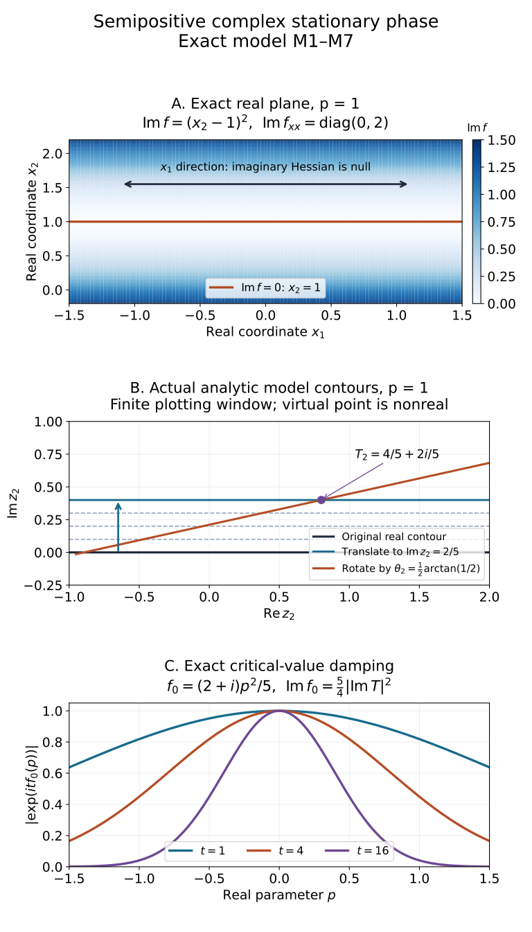
Open the full-size figure.

Figure 9.1. All panels depict the exact polynomial (M1)–(M3), not a schematic of the general almost-analytic construction (C1)–(C11). Panel A fixes $p=1$; $\operatorname{Im}f=(x_2-1)^2$ is constant in the null Hessian direction $x_1$. Panel B shows a finite plotting window in the complex $x_2$ plane. Translate the real contour through the horizontal lines $z_2=u+iy$, $0\le y\le2p/5$, for $p=1$. Along each line,

The final translated line passes through $T_2=(4+2i)p/5$. Then rotate its centered coordinate to $z_2=T_2+e^{i\theta_2}u_2$, with $0\le\theta_2\le\frac12\arctan(1/2)$. Independently rotate $z_1=e^{i\theta_1}u_1$, $0\le\theta_1\le\pi/4$. Completing the square gives

During these rotations the imaginary quadratic coefficients are respectively $\sin(2\theta_1)\ge0$ and $\sin(2\theta_2)+2\cos(2\theta_2)>0$. At the final product contour,

These are actual analytic contour deformations of the quadratic model. In the $z_2$ translation and rotation, end terms vanish by Gaussian decay. For the undamped $z_1$ direction take the Abel-regularized Fresnel limit of (B1), and then rotate its contour through the damped sector; the value and branch are fixed by (B2). The Jacobian is $e^{i\pi/4+i\theta_2}$; its second factor satisfies $e^{i\theta_2}5^{-1/4}=(2-i)^{-1/2}$ on the right-half-plane branch, recovering precisely (M3). Panel C plots the exact critical-value modulus

The plotted curves use $t=1,4,16$. They describe the full Gaussian model. A compact cutoff has the local expansion and rapid off-critical errors described after (M3), rather than the exact full-Gaussian integral. The reproducible figure source retains every coordinate and coefficient; outlined glyphs retain the complete DejaVu notice, STIX notice and BaKoMa notice.